Contents lists available atScienceDirect
Computers and Mathematics with Applications
journal homepage:www.elsevier.com/locate/camwaFL-GrCCA: A granular computing classification algorithm based on
fuzzy lattices
Hongbing Liu
a,b,∗, Shengwu Xiong
a, Zhixiang Fang
caSchool of Computer Science and Technology, Wuhan University of Technology, Wuhan 430070, PR China bDepartment of Computer Science, Xinyang Normal University, Xinyang 464000, PR China
cState Key Laboratory for Information Engineering in Surveying Mapping and Remote Sensing, Wuhan University, Wuhan 430079, PR China
a r t i c l e i n f o
Article history:
Received 17 October 2009
Received in revised form 24 October 2010 Accepted 24 October 2010 Keywords: Granule Granular computing Inclusion measure Fuzzy lattice
Positive valuation function
a b s t r a c t
Defining a relation between granules and computing ever-changing granules are two important issues in granular computing. In view of this, this work proposes a partial order relationand lattice computing, respectively, for dealing with the aforementioned issues. A fuzzy lattice granular computing classification algorithm, or FL-GrCCA for short, is proposed here in the framework of fuzzy lattices. Algorithm FL-GrCCA computes a fuzzy inclusion relation between granules by using aninclusion measurefunction based on both a nonlinear positive valuation function, namelyarctan, and an isomorphic mapping between lattices. Changeable classification granules are computed with a dilation operator using, conditionally, both the fuzzy inclusion relation between two granules and the size of a dilated granule. We compare the performance of FL-GrCCA with the performance of popular classification algorithms, including support vector machines (SVMs) and the fuzzy lattice reasoning (FLR) classifier, for a number of two-class problems and multi-class problems. Our computational experiments showed that FL-GrCCA can both speed up training and achieve comparable generalization performance.
©2010 Elsevier Ltd. All rights reserved.
1. Introduction
There have been many researchers working in the granular computing field. Zadeh has identified three basic concepts, namelygranulation,organization and causation, that underlie the process of human cognition [1,2]. More specifically, granulation is a process which decomposes a universe into parts. Conversely, organization is the way in which parts are integrated into the universe by the operation between two granules. Causation involves the association of causes and effects. Hobbs presented a framework for a theory of granularity and obtained the changeable granules in [3]. It enables us to map the complexities of the world around us into simple theories. From 1988 to 1996, Lin published articles on granular computing and neighborhood systems, mainly focusing on a granular computing model which included the binary relation, the granular structure, the granule’s representation, and the applications in granular computing [4–7]. Yao introduced rough sets to granular computing, and discussed data mining methods, rule extraction methods and machine learning methods based on granular computing in [8]. Liu defined granular logic, formed the corresponding inference system and successfully applied it in medical diagnosis [9]. It turns out that the relation between granules and the computation of changeable granules are two important issues in granular computing. This work proposes a partial order relation and lattice computing, respectively, for dealing with the two aforementioned issues.
∗Corresponding author at: School of Computer Science and Technology, Wuhan University of Technology, Wuhan 430070, PR China.
E-mail address:[email protected](H. Liu).
0898-1221/$ – see front matter©2010 Elsevier Ltd. All rights reserved.
A lattice is a partially ordered set in which any two elements have both a greatest lower bound and a least upper bound [10]. Lattice theory emerges naturally in granular computing because (information) granules are partially ordered. The termlattice computingwas introduced recently by Graña [11]. More specifically, lattice computing was defined as the class of algorithms that use lattice theory either to achieve pattern recognition or to produce generalizations. Graña and colleagues have applied lattice computing to image analysis [12,13]; moreover, they proposed an end member threshold selection algorithm (ETSA) [14]. The notion of afuzzy latticewas proposed by Nanda in 1989 on the basis of the concept of a fuzzy partial order relation [15]. In [16], Chakrabarty modified the definition of the fuzzy lattice after observing some redundancies in Nanda’s definition.
Fuzzy lattices have also been used in classifiers. More specifically, Kaburlasos and colleagues proposed a fundamentally new and inherently hierarchical approach in neurocomputing called fuzzy lattice neurocomputing (FLN) [17]. Note that FLN implements fuzzy lattice reasoning (FLR) classification, where a partial order relation is computed on the basis of a positive valuation function. Moreover, FLR classifiers were applied in air quality assessment [18] as well as in ambient ozone estimation [19].
The contribution of this work concerns mainly the application of a novel granular computing classification algorithm, namely FL-GrCCA, based on fuzzy lattices. Our algorithm consists of three steps. First, a granule is represented by two points (samples) including a beginning point and an end point inN-dimensional space. Note that a single point is treated as an atomic granule whose beginning point and end point coincide. Second, the nonlinear positive valuation functionarctanis introduced here for computing the inclusion measure function. Third, the inclusion measure of two granules is used, together with the size of a dilated granule, in the computations.
The layout of the remainder of this paper is as follows. Section2introduces the mathematical background. Section3 describes algorithm FL-GrCCA. Section4presents comparative experimental results. Finally, Section5summarizes our contribution and describes future work.
2. Mathematical background
A lattice
(
L,
≼
)
is a partially ordered set, such that any two of its elementsx,
y∈
Lhave a greatest lower bound xfy , inf{
x,
y}
and a least upper boundxgy , sup{
x,
y}
. A lattice(
L,
≼
)
is called complete when each of its subsets has a least upper bound and a greatest lower bound inL. A non-void complete lattice has a least element and a greatest element denoted byOandI, respectively [19]. For example, the real number setRis a complete lattice under the inequality relation≤
betweenx,
y∈
R, with the least element being−∞
and the greatest element being+∞
. Note that, in the context of this work, we assumestraightsymbols such as≤
,∧
,∨
between real numbers, whereas we assume curly symbols such as≼
,f,gbetween other lattice elements; e.g. 1≤
2, whereas[
1,
2] ≼ [
1,
3]
, etc.Suppose
(
L,
≼
)
and(
L,
≼
∂)
are lattices, where≼
and≼
∂≡ ≽
represent, respectively, their partial order relations;(
L,
≼
)
and(
L,
≼
∂)
aredual(to each other) sincex≼
yin(
L,
≼
)
is equivalent toy≽
xin(
L,
≽
)
. The least upper bound of a subsetLS in lattice(
L,
≼
)
is the greatest lower bound ofLSin lattice(
L,
≽
)
. For example, the lattice(
R,
≤
)
and lattice(
R,
≥
)
are dual, whereRdenotes the set of real numbers.Afuzzy latticeis a pair
⟨
L, µ
⟩
, where(
L,
≼
)
is a crisp lattice and(
L×
L, µ)
is a fuzzy set with membership functionµ
:
L×
L→ [
0,
1]
such thatµ(
a,
b)
=
1⇔
a≼
b.It turns out that disparate data types, including logic values, sets, symbols and graphs, are partially ordered. A popular practice in processing nonnumerical data is transforming them to numerical ones. For example, the symbol setL
=
{
good,
better,
best}
can be transformed to the numerical setS= {
60,
85,
100}
to be processed by the computer. Note that the ordering relation between two elements/numbers of the setS corresponds to the ordering relation between corresponding elements/symbols of the setL. More specifically, the ordering 60≤
85≤
100 in Scorresponds to the orderinggood≼
better≼
bestinL.A fuzzy relation between two objects in the transformed set may preserve the fuzzy relation between the corresponding two objects in the original set as follows. We define an order-preserving function
υ(
·
)
between lattices(
L,
≼
)
and(
R,
≤
)
such thatx≼
yimpliesυ(
x)
≤
υ(
y)
, forx,
y∈
L. Kaburlasos and colleagues have employed a positive valuation function as an order-preserving mapping [19].Avaluation functionis the order-preserving mapping
υ
:
L→
R,∀
a,
b∈
L,υ(
a)
+
υ(
b)
=
υ(
afb)
+
υ(
agb)
. If a valuation function satisfiesa≺
b⇔
υ(
a) < υ(
b)
, then the valuation function is called a positive valuation function. We denote these two properties as theequalityproperty and theinequalityone, respectively.For a complete latticeL, theinclusion measurefunction
σ
, namelyσ
:
L×
L→ [
0,
1]
,
by definition, satisfies the following four conditions,
∀
a,
b,
x∈
L:(1)
∀
a̸=
O, σ (
a,
O)
=
0, whereOis the least element of complete lattice(
L,
≼
)
; (2)σ(
a,
a)
=
1;(3)a
≼
b⇒
σ (
x,
a)
≤
σ (
x,
b)
; (4)afb≺
a⇒
σ (
a,
b) <
1.Theorem 1. If function
υ
:
L→
R is a positive valuation withυ(
O)
=
0in a lattice(
L,
≼
)
then the following two functions are inclusion measure functions[19,20]:k
(
a,
b)
=
υ(
b)
υ(
agb)
s(
a,
b)
=
υ(
afb)
υ(
a)
.
For lattice
(
L,
≼
)
, we can define the positive valuation function by using the sufficient conditionυ(
O)
=
0 mentioned in Theorem 1, where the equality property and inequality property must be satisfied.For the classification problem inN-dimensional space, in order to obtain (changeable) granules, the spaceRNis divided into granules with changeable size by the inclusion relation between two granules. Next, we discuss the inclusion relation between two granules which are represented by vectors in theN-dimensional spaceRN.
The partial order relation of two vectorsx
,
y∈
RN x=
(
x1,
x2, . . . ,
xN)
and y=
(
y1,
y2, . . . ,
yN)
isx
≼
y,(
x1≤
y1)
&(
x2≤
y2)
&. . .
&(
xN≤
yN)
where(
R,
≤
)
is a lattice.It is well-known that if
(
R,
≤
)
is a lattice, then(
R,
≼
)
N is a lattice too. In the two-dimensional spaceR2,∀
(
x,
y)
∈
R2 follows(
−∞
,
−∞
)
≼
(
x,
y)
≼
(
+∞
,
+∞
)
. That is,(
−∞
,
−∞
)
and(
+∞
,
+∞
)
are, respectively, the least and the greatest elements in lattice(
R,
≼
)
2.For lattice
(
R,
≤
)
, we define the partially orderedinterval setτ(
R)
asτ(
R)
= {[
a,
b]|
a,
b∈
Rwitha≤
b}
.
We remark that an interval is a granule in one-dimensional space. Furthermore, a single real numbera
∈
Rcorresponds to the trivial interval[
a,
a]
.A partial order relation is defined in
τ(
R)
as follows[
a,
b] ≼ [
c,
d]
,{
c≤
a,
b≤
d}
.
Operatorsgandfin the interval set
τ(
R)
are defined in the following.[
a,
b]
g[
c,
d]
,[
a∧
c,
b∨
d]
[
a,
b]
f[
c,
d]
,
[
a∨
c,
b∧
d]
ifa∨
c≤
b∧
d0 otherwise.
It is known that
(τ(
R),
≼
)
is a complete lattice, namely aninterval lattice, with least element[+∞
,
−∞]
and greatest element[−∞
,
+∞]
[19,20].We obtained two different lattices from lattice
(
R,
≤
)
: one is the interval lattice(τ(
R),
≼
)
, and the other one is the Cartesian product lattice(
R,
≼
)
2. On the one hand, for the interval lattice, if[
a,
b]
,
[
c,
d] ∈
τ(
R),
[
a,
b] ≼ [
c,
d]
, then[
a,
b] ∧ [
c,
d] = [
a,
b]
, namely[
a,
b] ∧ [
c,
d] = [
a∨
c,
b∧
d] = [
a,
b]
. Thereforea∨
c=
a,
b∧
d=
b, namelyc≤
a,
b≤
d. On the other hand, for the Cartesian product lattice(
R,
≼
)
2, if(
a,
b), (
c,
d)
∈
R2, (
a,
b)
≼
(
c,
d)
, thena≤
c,
b≤
d.The partial order relations in the interval lattice and in the Cartesian product lattice are contradictory becausec
≤
a in lattice(τ(
R),
≼
)
, whereasa≤
c in lattice(
R,
≼
)
2. Therefore, a dual isomorphic functionθ
is used to resolve the aforementioned contradiction according to the following equivalence: a≤
c⇔
θ(
a)
≥
θ(
c)
. Functionθ
must be a decreasing function. For instance, when the setRof real numbers is mapped onto the unit interval[
0,
1]
by function f(
x)
=
11+e−x, then function
θ
can be selected asθ(
x)
=
1−
x[19].As soon as an isomorphic function
θ
is defined, the partial order relations in the Cartesian product lattice and the interval lattice are related by the positive valuation function:υ
τ(
[
a,
b]
)
=
υ(θ(
a))
+
υ(
b)
(1)where
υ
τ(
·
)
is a valuation function on the interval lattice(τ(
R),
≼
)
, andυ(
·
)
is a positive valuation function in the lattice(
R,
≤
)
of real numbers.An inclusion measure function in the interval lattice
(τ(
R),
≼
)
can be computed as follows kτ(
[
a,
b]
,
[
c,
d]
)
=
υ
τ(
[
c,
d]
)
υ
τ(
[
a,
b]
g[
c,
d]
)
(2)sτ
(
[
a,
b]
,
[
c,
d]
)
=
υ
τ(
[
a,
b]
f[
c,
d]
)
3. FL-GrCCA: a granular computing classification algorithm based on fuzzy lattices
ForN-dimensional space, we construct our proposed algorithm in terms of the following steps. Firstly, two points in space are used to represent the granule, and each sample is regarded as the atomic granule which cannot be divided. Secondly, the nonlinear positive valuation function is introduced to make the interval space and the Cartesian space identical, and an inclusion measure function is formed to measure the inclusion relation between granules. Thirdly, the dilation operator is designed to update the granules.
The idea of FL-GrCCA is described as follows. For then-class classification problem, during the training process, the training set is divided intonsubsets by the class labels. Taking the subsetX1for example, a sample is selected to form the initial classification granule setGSDat random. For each samplex1i
∈
X1(
i=
1,
2, . . . ,
|
X1|
)
, we calculate the inclusion measureσ
ijbetween the samplex1i and each granuleGSDj(
j=
1,
2, . . . ,
|
GSD|
)
. If theGSDk includes the samplex1i maximally and the size of dilated granulex1i∨
GSDkis less than or equal to a user-defined parameter, thenGSDkis replaced by the dilated granulex1i∨
GSDk. Otherwise,x1iis used to form the new classification granule which becomes the new member ofGSD. After all the subsets are learned, the classification granule set is obtained. During the testing process, all the inclusion measures where the testing samplexbelongs to each classification granule inGSDare computed, and the corresponding class label with the maximal inclusion measure is assigned tox. The proposed algorithm FL-GrCCA is illustrated inAlgorithm: FL-GrCCA.Algorithm. FL-GrCCA
Input: the training set, the user-defined granule’s size
ρ
0Output: the classification granule set including changeable granules S1. initialize the classification granule setGS
=
∅S2. i
=
1S3. extract theith class sample and form the setXi
S4. initialize the class granule setGSD
=
∅for the setXi S5. j=
1S6. for thejth sample inXi, construct the atomic granuleGP0
S7. k
=
1S8. compute the inclusion measure, between the atomic granuleGP0and thekth granule in the class granule set GSD
σ (
k)
=
kτ(
GP0,
GSD(
k))
S9. k
=
k+
1S10. find the granuleGSD
(
id)
with the maximal inclusion measure in the class granule setGSD, where id=
arg maxkσ (
k)
S11. dilate the atomic granuleGP0intoGSD
(
id)
, and form the temporary granuleGSDtS12. GSD
(
id)
=
GSDt, if the size of temporary granule is less than or equal to the user-defined threshold (ρ
GSDt≤
ρ
0). Otherwise, add the temporary granuleGSDtto the class granule set.S13. j
=
j+
1S14. add the class labelito the class granule setGSD S15. update the classification granule setGS
=
GS∪
GSD S16. i=
i+
13.1. Representation and size definition for the granule
The training set is composed of
ℓ
N-dimensional input vectors andℓ
class labels. Two pointsx=
(
x1,
x2, . . . ,
xN)
andy
=
(
y1,
y2, . . . ,
yN)
are used to represent the granule. The form of the granule isG=
(
x,
y)
T, wherex≼
y. Here, pointx is called the beginning point, andyis called the end point. For example, in two-dimensional space,G= [
0.
1,
0.
2,
0.
4,
0.
6]
represents the granule which has the beginning point(
0.
1,
0.
2)
and the end point(
0.
4,
0.
6)
. The length of granuleGequals 0.4, and its width equals 0.3. Another example is the atomic granule(
3,
4,
3,
4)
T, which represents the single point(
3,
4)
.The distance between the beginning pointxand the end oneyis used to define the granule’s size. The formula for the distance is
ρ
= ‖
x−
y‖ =
p
N−
i=1|
xi−
yi|
p (4)wherex
=
(
x1,
x2, . . . ,
xN),
y=
(
y1,
y2, . . . ,
yN)
∈
RN.ρ
can be the Manhattan distance (forp=
1), Euclidean distance (forp
=
2), or Chebyshev distance (forp= ∞
). The positive valuation function(1)can also be used to define the granule’s size [19]ρ
=
N−
i=1υ(
[
xi,
yi]
)
wherex=
(
x1,
x2, . . . ,
xN),
y=
(
y1,
y2, . . . ,
yN)
∈
RN.3.2. The inclusion measure function
In Section2, the inclusion measure functions given by(2)and(3)were defined on the basis of the positive valuation function (1). Note that Kaburlasos and Petridis have extensively employed linear positive valuation functions in the N-dimensional space
[
0,
1]
N [21]. Nevertheless, the transformation from a symbol set to the real number set may be nonlinear. For example, for the symbol setL= {
good,
better,
best}
and the real number setR= [
0,
1]
, if we suppose goodis mapped into 0.6, thenbetter may be mapped into 0.
612=
0.
7746 andbestmay be mapped into 0.
613=
0.
8434 by the nonlinear mappingsx12 andx1
3. We define a nonlinear positive valuation function which valuates the partial order relation in the spaceRinstead of in the spaceLas follows
υ(
x)
=
1π
arctanx+
1
2
.
(5)On the basis of the complete lattice
(
R,
≤
)
,∀
a,
b∈
R, a,
b are comparable, namelya∧
b=
a,
a∨
b=
b or a∧
b=
b,
a∨
b=
a. Therefore,υ(
a)
+
υ(
b)
=
υ(
a∧
b)
+
υ(
a∨
b)
, and the aforementioned function(5)satisfies the equality property. Moreover, an increasing functionυ(
x)
, such thata<
b⇔
υ(
a) < υ(
b)
, satisfies the inequality property. Because−∞
is the least element of lattice(
R,
≤
)
andυ(
−∞
)
=
1π
arctan(
−∞
)
+
1 2= −
1π
·
π
2+
1 2=
0the valuation function(5)satisfies the sufficient condition
υ(
O)
=
0 mentioned inTheorem 1. Hence, function(5)is an eligible positive valuation function.After obtaining the positive valuation function(5), we can define the inclusion measure function on the interval lattice as follows
σ
τ(
[
a,
b]
,
[
c,
d]
)
=
υ
τ(
[
c,
d]
)
υ
τ(
[
a,
b]
g[
c,
d]
)
(6)where
υ
τ(
[
a,
b]
)
=
υ(θ(
a))
+
υ(
b)
andθ(
x)
=
1−
x, for the interval[
a,
b]
.The previous results are extended toN-dimensional space, next we discuss the inclusion measure function in the interval lattice
(τ(
R),
≼
)
inN-dimensional space.Theorem 2. If
(τ(
R),
≼
)
is a fuzzy lattice, then(τ(
R)
N,
≼
)
is a fuzzy lattice. The inclusion measure function of the fuzzy lattice(τ(
R)
N,
≼
)
isσ
kτ(
G1,
G2)
=
υ
τ(
G2)
υ
τ(
G1gG2)
where G1,
G2∈
τ(
R)
N.We remark that function
σ
kτ(
·
,
·
)
ofTheorem 2is used exclusively in our numerical experiments, below we will discusshow to dilate granules by using the inclusion measure between granules. 3.3. The dilation operator of granules
On the basis of the inclusion measure function given by(6), we can compute the inclusion relation between two granules. In two-dimensional space, in particular,
τ(
R)
×
τ(
R)
is the Cartesian product lattice of two interval lattices. Hence, the inclusion measure can be computed by using(6), where thegoperator computes the dilation of (information) granules. Note that the dilation operator (g) has been used widely in the fields of classification, neural networks, and machine learning, in the context of mathematical morphology [22–25]. In the following, we demonstrate the computation of the inclusion measure function(6)on the plane.As shown inFig. 1, pointP0
(
0.
45,
0.
5)
lies inside the granule G= [
0.
43588,
0.
4077,
0.
50009,
0.
53541]
and the inclusion measure ofP0belonging toGis
σ(
P0≼
G)
=
υ(
1
−
0.
43588)
+
υ(
0.
50009)
+
υ(
1−
0.
4077)
+
υ(
0.
53541)
υ(
1−
0.
43588)
+
υ(
0.
50009)
+
υ(
1−
0.
4077)
+
υ(
0.
53541)
=
1.
The inclusion measure of the outside pointP1(
0.
51,
0.
45)
belonging to the granuleGisσ(
P1≼
G)
=
υ(
1
−
0.
43588)
+
υ(
1−
0.
4077)
+
υ(
0.
50009)
+
υ(
0.
53541)
0.44 0.45 0.46 0.47 0.48 0.49 0.5 0.51 0.52 0.42 0.44 0.46 0.48 0.5 0.52 0.54 P0 P1 G
Fig. 1. The inclusion relation between atomic granules and a granule. The inclusion measure of the inside pointP0belonging to the granuleGis 1, and the
inclusion measure of the outside pointP1belonging to the granuleGis less than 1.
Fig. 2. Dilation of the atomic granule and granule. The dashed rectangleGis the granule, and the solid rectangleG′is the dilated granule ofGand pointP, the granule and its dilated granule have the same beginning point.
During the training process, a training datum is dilated into the granule if both the granule includes the data maximally and the size of the dilated granule is less than or equal to a user-defined threshold
ρ
0. The dilation operator is formed by using the method described in [26]. For two-dimensional space, letx=
(
x1,
x2)
andy=
(
y1,
y2)
be the beginning point and the ending point of a granuleG, and let pointPbeP=
(
a,
b)
∈
G. Then, the corresponding dilated granule is computed asG′=
[
x,
y]
gP= [
x∧
P,
y∨
P]
. For example, the dilated granule between granuleG= [−
0.
46502,
−
0.
33226,
0.
62899,
1.
8431]
and pointP=
(
0.
81,
2.
1)
isG′= [−
0.
46502,
−
0.
33226,
0.
81,
2.
1]
as shown inFig. 2.3.4. Discussion of FL-GrCCA
The size of a granule is the key parameter for computing changeable granules. We can perform the dilation process until all the training data with the same class label lie in the same granule. But our experimental results have shown that the method is only valid for some special classification cases, that is when either the classification margin between different classes is very large or training data with identical labels lie in a granule. For nonlinearly separable problems, the classification accuracy is poor. Therefore, we dilate the granules conditionally by introducing a threshold to control the size of the granule. The conditional dilation process results in changeable granules. In order to select the parameter of granule’s size expediently, all the training data are normalized into space
[
0,
1]
N by the functionX(
:
,
i)
=
X(
:
,
i)/
max(
X(
:
,
i))
,Table 1
Performance for the two-class problem.
Algorithms ρ0 Size Tr (%) Ts (%) Tr (s) Ts (s)
FL-GrCCA 0.03 208 100 100 5.8906 3.9531
FLR 0.1 240 100 100 5.875 4.0313
SVMs0.1 – – 100 100 10.0281 0.03125
i
=
1,
2, . . . ,
N. After the normalization, the maximal distance of any two training samples is not greater thanNin the space[
0,
1]
N. Therefore, in our experiments,ρ
0was selected from 0.
5Ndown to 0 in steps of 0.01.Regarding computational complexity, note that FL-GrCCA learns the training set in a single pass. The worst case training scenario is when all the training data are classification granules. In the latter case, FL-GrCCA learns the training data set and scans the classification granule set simultaneously. Hence, the training complexity isO
(ℓ
2)
, whereℓ
is the size of the training data set [27].4. Numerical experiments
We evaluated the effectiveness of our algorithm FL-GrCCA for both two-class problems and multi-class problems, with an Intel PIV PC with 2.8 GHz CPU and 512 MB memory, running Microsoft Windows XP professional and Matlab 7.0. 4.1. Two-class problems
The spiral classification is a difficult problem to be classified, and used to evaluate the performance of classifiers. The training data are generated by the method proposed in [28].
Rn
=
0.
4(
105−
n)/
104α
n=
π(
n−
1)/
16an
=
Rnsin(α
n+
q·
randn(
1,
1)/
100)
+
0.
5bn
=
Rncos(α
n+
q·
randn(
1,
1)/
100)
+
0.
5wheren
=
1,
2, . . . ,
97. The first class data are(
ai,
bi)
97i=1, and the second class data are(
1−
ai,
1−
bi)
i97=1.randn(
1,
1)
is the random number where the mean is 0 and the variance equals 1.qis the parameter which can tune the classification margin. We setq=
8 and generate six groups of spiral data; the first five groups are used for training, whereas the sixth group is used for testing. The two-class problem includes 970 training data and 194 testing data.The size of a granule is computed by using formula(4), forp
= +∞
andp=
1, moreover the thresholds are sorted in a descending order:ρ
0=
0.
2,
0.
1,
0.
09, . . . .
We performed FLR and FL-GrCCA with sizesp= +∞
andp=
1, and then found that the granule’s sizep=
1 produces better training/testing results. The maximalρ
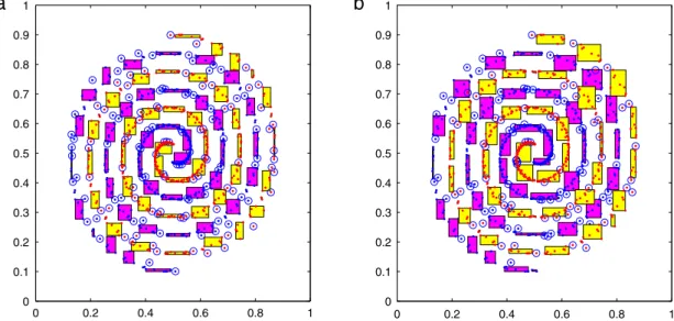
0which gave training accuracy is first selected in our experiments. The performance parameters, including the size of the classification granule set (size), training accuracy (Tr (%)), testing accuracy (Ts (%)), training time (Tr (s)), and testing time (Ts (s)), are listed inTable 1.Fig. 3 shows the changeable granules obtained by using FL-GrCCA and FLR classifiers [27]. There are 240 classification granules induced by FLR (Fig. 3(a)) withρ
0=
0.
1 and 208 classification granules induced by FL-GrCCA (Fig. 3(b)) withρ
0=
0.
03. Note that FL-GrCCA performed better than FLR since FL-GrCCA has resulted in fewer classification granules while retaining similar classification accuracy.Table 1shows that FL-GrCCA achieved its best performance for the threshold equal to 0.03. Larger threshold values resulted in larger size granules, moreover the classification accuracy deteriorated.We also compared FL-GrCCA with the popular learning algorithm SVMs
δ
, with the parametersC=
5000 and Gaussian kernelδ
=
0.
1 (http://asi.insa-rouen.fr/enseignants/~arakotom/toolbox/index.html). The training accuracies and testing accuracies were 100%, again. For SVMs, we tuned the parameter of the kernel function many times in order to achieve the best classification accuracy. For the spiral problem, SVMs with Gaussian kernels had a satisfactory performance, whereas the performance of SVMs with dot product kernels and polynomial kernels was poor.FromTable 1, we can see FL-GrCCA and FLR are faster than SVMs during the training process, while FL-GrCCA and FLR is slower than SVMs for testing process. The reason is that the decision function of SVMs is the analytical formula which determines the class of the testing sample directly, while FL-GrCCA determines the class of the testing sample by computing the inclusion measure between the testing sample and each classification granule. Nevertheless, for SVMs, we must tune more parameters includingC,
δ
and kernel functions; whereas, for FL-GrCCA and FLR, there is only one parameterρ
0that controls the size of the granule.4.2. Multi-class problems
For multi-class problems, the data sets in two-dimensional space andN-dimensional space are discussed in this section. For two-dimensional space, Grdata2000 and Grdata4000 are used to test the performance of our algorithm. The data set named Grdata2000 includes 2000 training data and 2000 testing data in four classes lying in the area
[
0,
2] × [
0,
2]
with a0 0.2 0.4 0.6 0.8 1 0 0.1 0.2 0.3 0.4 0.5 0.6 0.7 0.8 0.9 1 0 0.2 0.4 0.6 0.8 1 0 0.1 0.2 0.3 0.4 0.5 0.6 0.7 0.8 0.9 1
Fig. 3. The classification granules of the spiral problem. (a) shows 240 classification granules for FLR (ρ0=0.1), and (b) shows 208 classification granules
for FL-GrCCA (ρ0=0.03). 0 0.5 1 1.5 2 0 0.2 0.4 0.6 0.8 1 1.2 1.4 1.6 1.8 2 0 0.5 1 1.5 2 0 0.2 0.4 0.6 0.8 1 1.2 1.4 1.6 1.8 2
b
a
Fig. 4. Distributions of Grdata2000 (a) and Grdata4000 (b).
uniform distribution (Fig. 4(a)). Grdata4000 is an eight-class problem composed of 4000 training data and 4000 testing data (seeFig. 4(b)).
Furthermore, three benchmark data sets, includingiris,wineandimage, from a popular machine learning database (http://mlr.cs.umass.edu/ml/datasets.html), were selected to verify comparatively the capacity of our proposed algorithm. Table 2lists the data sets employed. For theirisandwinedata sets we list neither a testing data accuracy nor a testing time because the aforementioned data sets include only training data. We used the distance formula(4)(withp
=
1) to measure a granule’s size. In our experiments, we setρ
0from 0.
5Ndown to 0 in steps of 0.01. We compared FL-GrCCA with the SVMs and FLR classifiers.Table 3shows the performances of these three classification algorithms. FromTable 3we can see that FL-GrCCA can obtain not only better training accuracies but also better testing accuracies compared with SVMs. For example, Tr (%) and Ts (%) are 100% and 99.95% by using FL-GrCCA on Grdata2000, while Tr (%) and Ts (%) are 99.95% and 99.65% by using SVMs with Gaussian kernelδ
=
5 on Grdata2000.FromTable 3, we can also see that FL-GrCCA and FLR are comparable. For GrData2000, all the training data with the same class label lie in the same granule (square), four granules were obtained by FL-GrCCA and FLR without the parameter (size) and guaranteed the maximal training accuracy and testing accuracy. FLR achieved the optimal training accuracy ahead of FL-GrCCA. Foriris, FL-GrCCA’s training accuracy is 94.667%, whereas FLR’s training accuracy is 100% with the same granule size
ρ
0=
0.
9. For the generalization performance, FL-GrCCA is better than FLR for the data setimagewith the granule sizesTable 2
The testing data sets of multi-class problems.
Data sets No. of inputs No. of classes No. of training data No. of testing data
Grdata2000 2 4 2000 2000 Grdata4000 2 8 4000 4000 iris 4 3 150 – wine 13 3 178 – image 19 7 210 2100 Table 3
Performances for multi-class problems.
Data sets Classifiers ρ0 Size Tr (%) Ts (%) Tr (s) Ts (s)
FL-GrCCA – 4 100 99.95 0.51563 0.875 Grdata2000 FLR – 4 100 99.95 0.42188 0.73438 SVMs5 – – 99.95 99.65 4.5938 0.0625 FL-GrCCA 0.04 859 99.3 96.6 25.906 339.36 FL-GrCCA 0.02 1220 99.675 97.575 35.25 480.03 Grdata4000 FLR 0.04 1682 100 97.675 42.406 588.53 FLR 0.02 2246 100 97.675 55.406 786.16 SVMs0.01 – – 100 92.15 1032.5 16.813 FL-GrCCA 1.06 3 94.667 – 0.03125 – FL-GrCCA 0.24 18 100 – 0.0625 – iris FLR 1.06 19 100 – 0.0625 – FLR 0.24 86 100 – 0.21875 – SVMs0.01 – – 100 – 0.70313 – FL-GrCCA 6.25 3 97.753 – 0.046875 – FL-GrCCA 1.52 32 100 – 0.10938 – wine FLR 6.25 30 100 – 0.09375 – FLR 1.52 144 100 – 0.42188 – SVMs100 – – 100 – 1.2188 – FL-GrCCA 0.64 106 100 91.429 0.23438 29.563 FL-GrCCA 0.53 113 100 92.476 0.25 31.203 image FLR 0.64 160 100 90.571 0.3125 35.891 FLR 0.53 167 100 90.667 0.29688 37.297 SVMs50 – – 100 92.143 1.3594 0.5625
and
ρ
0=
0.
02. The size of the classification granule set obtained by FL-GrCCA is less than that obtained by FLR for the data setiris, whereas the size obtained by FLR is less than that obtained by FL-GrCCA for the data setwinewith the optimal training accuracy.5. Conclusion
A new classification algorithm, namely FL-GrCCA, was presented here in the framework of fuzzy lattices. FL-GrCCA induces classification granules, where a granule is characterized by a beginning point, an end point and a class label. Compared with alternative classification algorithms, including SVMs and FLR, FL-GrCCA has demonstrated both a better data-processing speed and a similar classification accuracy for a number of two-class problems as well as multi-class problems.
For future work we plan, firstly, to carefully choose parameterpin(4), secondly, to consider different inclusion measure functions and, thirdly, to study the stability of learning in alternative classification problems.
Acknowledgements
The authors would like to thank the anonymous reviewers and Ms. Xiaoxiao Niu for their helpful comments and discussion. This work was supported in part by the National Natural Science Foundation of China (Grant No. 40701153, 40971233), Natural Science Foundation of Henan Province (102300410178, 2009B520025) and self-determined and innovative research funds of WUT.
References
[1] L.A. Zadeh, Fuzzy sets and information granulation, in: Advances in Fuzzy Set Theory and Applications, North Holland Publishing, 1979.
[2] L.A. Zadeh, Towards a theory of fuzzy information granulation and its centrality in human reasoning and fuzzy logic, Fuzzy Sets and Systems 19 (1997) 111–127.
[3] J.R. Hobbs, Granularity, in: Proceedings of the Ninth International Joint Conference on Artificial Intelligence, Los Angeles CA, August 18–23, 1985, pp. 432–435.
[4] T.Y. Lin, Neighborhood systems and relational database, in: Proceedings of the ACM Sixteenth Annual Conference on Computer Science, New York, February 23–25, 1988, p. 725.
[5] T.Y. Lin, Data mining and machine oriented modeling: a granular computing approach, Journal of Applied Intelligence 13 (2) (2000) 113–124. [6] T.Y. Lin, Granular computing rough set perspective, The Newsletter of the IEEE Computational Intelligence Society 2 (4) (2005) 1543–4281. [7] T.Y. Lin, Granular computing: a problem solving paradigm, in: Proceedings of the IEEE International Conference on Fuzzy Systems, Reno, Nevada, USA,
May 22–25, 2005, pp. 132–137.
[8] Y.Y. Yao, Information granulation and rough set approximation, International Journal of Intelligent Systems 16 (1) (2001) 87–104. [9] Q. Liu, Z.H. Huang, G-logic and its resolution reasoning, Chinese Journal of Computers 27 (7) (2004) 865–872.
[10] G. Birkhoff, Lattice Theory, American Mathematical Society, Providence, Rhode Island, 1967.
[11] M. Graña, A brief review of lattice computing, in: Proceedings of the World Congress on Computational Intelligence, Hong Kong, China, June 1–6, 2008, pp. 1777–1781.
[12] M. Graña, A.M. Savio, M. García-Sebastián, E. Fernádez, A lattice computing approach for on-line fMRI analysis, Image and Vision Computing 28 (7) (2010) 1155–1161.
[13] M. Graña, M. García-Sebastián, C. Hernández, Lattice independent component analysis for fMRI analysis daft slides, Lecture Notes in Computer Science 5768 (2009) 725–734.
[14] M. Graña, I. Villaverde, J.O. Maldonado, C. Hernández, Two lattice computing approaches for the unsupervised segmentation of hyperspectral images, Neurocomputing 72 (10–12) (2009) 2111–2120.
[15] S. Nanda, Fuzzy lattices, Bulletin Calcutta Mathematical Society 81 (1989) 1–2.
[16] K. Chakrabarty, On fuzzy lattice, Lecture Notes in Artificial Intelligence 2001 (2005) 238–242.
[17] V.G. Kaburlasos, V. Petridis, Fuzzy Lattice Neurocomputing (FLN): a novel connectionist scheme for versatile learning and decision making by clustering, International Journal of Computers and Their Applications 4 (3) (1997) 31–43.
[18] I.N. Athanasiadis, V.G. Kaburlasos, Air quality assessment using Fuzzy Lattice Reasoning (FLR), in: Proceedings of IEEE International Conference on Fuzzy Systems, Vancouver, BC, Canada, July 16–21, 2006, pp. 29–34.
[19] V.G. Kaburlasos, I.N. Athanasiadis, P.A. Mitkas, Fuzzy Lattice Reasoning (FLR) classifier and its application for ambient ozone estimation, International Journal of Approximate Reasoning 45 (2007) 152–188.
[20] V.G. Kaburlasos, Towards a unified modeling and knowledge-representation based on lattice theory: computational intelligence and soft computing applications, in: Studies in Computational Intelligence, Springer-Verlag New York Inc., 2006.
[21] V.G. Kaburlasos, V. Petridis, Fuzzy Lattice Neurocomputing (FLN) models, Neural Networks 13 (10) (2000) 1145–1170.
[22] M.E. Valle, P. Sussner, A general framework for fuzzy morphological associative memories, Fuzzy Sets and Systems 159 (7) (2008) 747–768. [23] A.M. da Silva, P. Sussner, A brief review and comparison of feedforward morphological neural networks with applications to classification, Lectures
Notes in Computer Science 5164 (2008) 783–792.
[24] P. Sussner, E.L. Esmi, An introduction to morphological perceptrons with competitive learning, in: Proceedings of International Joint Conference on Neural Networks, IJCNN 2009, Atlanta, Georgia, 2009, pp. 3024–3031.
[25] P. Sussner, E.L. Esmi, Constructive morphological neural networks: some theoretical aspects and experimental results in classification, in: L. Franco, D.A. Elizondo, J.M. Jerez (Eds.), Constructive Neural Networks, Studies in Computational Intelligence 258 (2010), 123–144.
[26] G.A. Carpenter, S. Grossberg, N. Markuzon, J.H. Reynolds, D.B. Rosen, Fuzzy ARTMAP: a neural network architecture for incremental supervised learning of analogy multidimensional maps, IEEE Transactions on Neural Networks 3 (5) (1992) 698–713.
[27] V.G. Kaburlasos, S.E. Papadakis, A granular extension of the Fuzzy-ARTMAP (FAM) neural classifier based on Fuzzy Lattice Reasoning (FLR), Neurocomputing 72 (2009) 2067–2078.