Quantifying optimal capital allocation principles based on risk measures

(1)

Title: Quantifying Optimal Capital Allocation Principles

based on Risk Measures.

Author: Jilber Andrés Urbina Calero.

Advisor: Montserrat Guillén.

Department: Statistics and Operations Research.

University: Universitat Politènica de Catalunya

Academic year: 2013

Interuniversity Master

in Statistics and

Operations Research

(2)

Universitat Politècnica de Catalunya

Master Thesis

Quantifying Optimal Capital Allocation Principles based on Risk

Measures.

Author:

Jilber Andrés Urbina Calero

Supervisor: Montserrat Guillén

Department:

Statistics and Operations Research

Thesis submitted to the faculty of Mathematics and Statistics of Universtitat Politècnica de Catalunya

in partial fulfillment of the requirements for the degree of MASTER OF SCIENCE

in

(3)

Abstract

In this thesis we address the issue of covering risks by allocating capital and solving the so-called allocation problem. For this purpose, we provide functional closed-forms representations for each allocation principle built under the general framework devel-oped by Dhaene et al. (2012). Furthermore, we assess the correlation effect which is considered to be the effect of changes in the allocated capital when changing the correlation between the losses, this effect arises when the sources of risk have different variances, otherwise correlations does not play any role in capital allocation results. We develop an R package called OCA which computes optimal Capital Allocations based on some standard principles such as Haircut, Overbeck type II and the Covari-ance Allocation Principle. Also it provides some functionalities for estimating two of the most popular risk measures: Value at Risk and Expectation Shortfall.

Keywords: Risk, Risk management, Optimal Capital Allocations, Allocation Principles, Value-at-Risk, Expected Shortfall

(4)

Notation

E(·) Expected Value operator.

Xi Random variables with finite mean representing individual losses.

S Aggregate loss defined asPN

i=1Xi.

ρ(·) A mapping function representing a risk measure.

Ki Non-negative real numbers representing individual capital to be allocated to thei-th

business unit, i= 1, . . . , N.

K Aggregate capital to be split into Ki individual parts based on different forms of ρ(·).

VaR Value at Risk.

ES Expected Shorfall.

CTE Conditional Tail Expectation.

r.v. Random variable.

Γ A real-valued random variable defined on a probability space (Ω,F,P).

Ω Sample space.

F Set of all possible events (a σ-algebra).

P Probability.

inf Infimum.

p Probability such thatp∈(0,1).

FXi(x) Probability distribution function of a r.v. X defined asP(Xi ≤x). F_X−1

i(p) Inverse of the distribution function, it is called the quantile function.

Φ Standard normal distribution function.

Φ−1(p) The p-th quantile ofΦ.

φ Density of a standard normal distribution.

µ Expected value of a r.v.

V ar(·) Variance of a r.v.

σ2 Variance of a r.v.

σ Standard deviation of a r.v.

Cov(x, y) Covariance between two r.v.’s.

tυ Distribution function of a standard t with υ degrees of freedom. t−_υ1(p) The p-th quantile oftυ.

gυ(·) Density of a standard t-distribution withυ degrees of freedom.

I(·) Indicator function that takes the value 1 if condition in (·)is met, and takes the

value zero otherwise.

υi Measure of risk exposure.

(5)

List of Tables

1 Business Unit Driven Capital Allocation . . . 21

2 Aggregate Portfolio Driven Allocations . . . 26

3 Descriptive statistics for numerical example data . . . 27

4 Case I. Capital allocation based on different principles . . . 28

5 Case I. Proportions of capital allocation based on different principles . . . 29

6 Case II. Capital allocation based on different principles. . . 30

7 Case II. Proportions of capital allocation based on different principles. . . 31

8 Simulation results Case I. . . 32

(7)

1 Introduction

Risk management, among other tasks, evaluates the total capital requirements of a company and allocates it to its various business units. A natural question is: how should a given a mount of capital be allocated among the different business lines belonging to a company? To accomplish this, several allocation principles have been developed in the literature, most of them are based on risk measures sourced either by internal or external factors of the company.

Companies wish to allocate capital to their business units for solvency reasons, i.e. banks and insurance companies are legally required to set aside some amount of capital in order to remain solvent. Also capital allocation can be a useful tool for performance measurement and designing incentives schemes as managers’ performance can be assessed by the amount of capital allocated to their business units. Profit-and-loss analysis under loan pricing context and under general investment purposes are another reasons that motivate companies to carry out capital allocations.

Covering risks by allocating capital is the target of this thesis1 and the main problem to be solved is the so-called allocation problem. Based on the general framework proposed by Dhaene et al.(2012) we provide explicit formulations for the proportion of capitals the manager should allocate on different risk sources based on a wide variety of risk measures.

In this thesis we are particularly interested in providing the exact functional forms of each allocation principle and also paying carefully attention to the numerical part, we analyse the “correlation effect” on the allocation principles. Correlation effect is considered to be the effect of changes in the allocated capital suggested by each principle when changing the correlation between the losses.

Our findings suggest thatcorrelation effectdoes not play any role when losses are characterized by the same two distributional moments (mean and variance), nevertheless when variances differ while means remain the same some important differences arise when correlation goes from 0 to 1 leading to a clearcorrelation effect.

This thesis has entirely developed an R package, which has been called OCA package. This package computes Optimal Capital Allocations (OCA) based on some standard principles such as Haircut, Overbeck type II and the Covariance Allocation Principle. Also it provides some short-cuts for obtaining two of the most popular risk measures: Value at Risk and Expectation Shortfall.

The remainder of this thesis is arranged as follows: section 2 discusses formally what the allocation problem is,section 3characterizes coherent risk measures by providing its properties, then section 4 presents some well-know risk measures. Allocation principles are presented in

section 5 while the general framework for capital allocation, based on Dhaene et al. (2012), is discussed in section 6. Numerical applications and simulations are reported in section 7 and

section 8. Some concluding remarks are in section 9. The manual forOCA package as well as the R codes for reproducibility of this work are presented insection 10.

1

Note that capital allocation is the purpose of this work and we do not attempt going into details on how to determine the economic capital to be allocated. We assume this capital is known and given, we are after a way to determine the optimal proportions of this given capital for allocating them among different risk sources of the enterprise.

(8)

2 The Allocation Problem

Capital Allocation is a term referring to the subdivision of the aggregate capital held by the firm across its various constituents, for example, business lines, type of exposure, territories, or even individual products in a portfolio of insurance policies. This capital is often referred to as Economic Capital (EC) and is defined as the p-quantile of the loss distribution minus the expected value of the of loss distribution (Overbeck,2000), formally this is:

EC(p) =F_X−1

i(p)−E(S) with,

F_S−1(p) = inf{x∈_R|FS(s)≥p}, p∈(0,1).

Since this definition ofEC(P) does not account for“bad times” episodes, then it is viewed as an “all or nothing” rule for capital definition. An alternative definition, according to Overbeck

(2000), tries to incorporate such“bad times” in its formulation and treat it as a more“optimistic” event, this definition states thatEC must be:

ECK =E(S|S > K),

where this definition considers Economic Capital in average also enough to cushion losses even in bad times. Note that capital allocations insubsubsection 6.2.2are based on this capital definition. Once the capital is defined, we have to define its counterpart, the loss. Consider a portfolio of n individual losses (random variables)X1, X2, . . . , Xn materializing at a fixed future date T.

Assume that(X1, X2, . . . , Xn)is a random vector on the probability space(Ω,F,P). Throughout

this thesis, we will always assume that any loss Xi has a finite mean. The distribution function P(Xi≤x) ofXi will be denoted byFXi(x).

The aggregate loss is defined by the sum of the individual losses:

S=

n

X

i=1

Xi, (1)

where this aggregate loss can be interpreted as:

1. the total loss of a corporation, for example, an insurance company, with the individual losses corresponding to the losses of the respective business unit,

2. the loss from an insurance portfolio, with the individual losses being those arising from the different policies; or

3. the loss by a financial conglomerate, white the different individual losses correspond to the losses suffered by its subsidiaries.

Following Dhaene et al. (2012) it is the first of these interpretations we will use throughout this thesis.

Hence, S is the aggregate loss faced by an insurance company and Xi is the loss of business

(9)

In order to clarify what the allocation problem is, one can view the problem from another perspective, namely, consider an investor who can invest in a fixed set of n different invest-ment possibilities with losses represented by the random variablesX1, X2, . . . , Xn. We have the

following economic interpretations depending on the area of application (McNeil et al.,2005): 1. Performance measurement. Here the investor is a financial institution and the Xi

represent the Profit-and-Loss distribution ofndifferent lines of business.

2. Loan pricing. In this situation the investor is a loan book manager responsible for a portfolio ofn loans.

3. General investment. Here we consider either an individual or institutional investor and the standard interpretation ofXi are profit-and-loss corresponding to a set of investments

in various assets.

S is random, so usually we assume that the company has already determined the aggregate level of capital safely to face those losses and denote this total risk capital by K. The company now wishes to allocate this exogenously given total risk capital K across its various business units, that is, to determine non-negative real numbers K1, . . . , Kn satisfying the full allocation

requirement:

n

X

i=1

Ki=K. (2)

This allocation is in some sense a notional exercise; it does not mean that capital is physically shifted across the various units, as the company’s assets and liabilities continue to be pooled. The allocation exercise could be made in order to rank the business units according to levels of profitability. This task can be performed, for example, by determining the returns on the allocated capital for the respective business units.

The general approach of capital allocation raises the question of what the appropriate risk capital for an individual investment opportunity might be. Thus the question of performance of the investment is intimately connected with the risk measurement chosen. A two-step procedure is used in practice (McNeil et al.,2005).

1. Compute the overall risk capitalρ(S), whereSis defined inEquation 1andρis a particular risk measurement such as VaR or ES (see section 4 for detailed explanation on these and other measures). Coherent measures will be more appropriate than non-coherent ones2 2. Compute K as ρ(S) and allocate the capital K to the individual investment possibilities

according to some mathematicalcapital allocation principle such that, if(Ki) denotes the

capital allocated to the investment with potential loss Xi. The sum of Ki fulfils the

re-quirement in Equation 2.

(10)

Throughout this study we are interested in the second step of the procedure pointed out above; roughly speaking we require a mapping that takes as input the individual lossesX1, X2, . . . , Xn

and the risk measureρ and yields as output the vector (K1, K2, . . . , Kn) such that:

ρ(S) =

n

X

i=1

Ki =K. (3)

Such a mapping will be called a capital allocation principle. The relation Equation 3 is sometimes called the full allocation property (McNeil et al., 2005) since all of the overall risk capitalρ(S)(not more, not less) is allocated to the investment possibilities; McNeil et al.(2005) consider this property to be an integral part of the definition of an allocation principle.

Given that a capital allocation can be carried out in a countless number of ways, additional criteria must be set up in order to determine the most suitable. A reasonable start is to require the allocated capital amountsKi to be “close” to their corresponding lossesXi in some appropriately

defined sense. This underlies the approach proposed in the present thesis. Prior to introducing the idea of “closeness” between individual loss and allocated capital, we revisit some well-known capital allocation methods. But before going into capital allocation methods it is worth to discuss about what a coherent risk measure is.

3 Coherent Risk Measures: Definition and Properties

A risk measure is a mappingρfrom a setΓof real-valued random variables defined on a probability space(Ω,F,P)to the real line R:

ρ: Γ→_R:X∈Γ→ρ[X]. (4)

The random variable X refers to the loss associated with conducting a business and ρ[X] represents the amount of capital to be set aside in order to make the loss X an acceptable risk.

Some well-know properties that risk measures may or may not satisfy are law invariance, monotonicity, positive homogeneity, translation invariance (or equivalence), and subadditivity, these axioms were proposed for applications in financial risk management in the seminal paper by Artzner et al.(1999). These axioms are formally defined as:

1. Law invariance: For any X1, X2 ∈ Γ with P[X1 ≤ x] = P[X2 ≤x]for all x ∈R, ρ[X1] = ρ[X2]

2. Subadditivity: For anyX1, X2 ∈Γ,ρ[X1+X2]≤ρ[X1] +ρ[X1]

The rational behind this is summarized byArtzner et al. (1999) in the statement that “a merger does not create extra risk”. McNeil et al. (2005) refer to subadditivity as the most debated of the axioms for a risk measure to be considered coherent,3 but also they provide some reasons why this axiom is indeed a reasonable requirement:

• Subadditivity reflects the idea that risk can be reduced by diversification, a time-honoured in finance and economics.

3

(11)

• If a regulator uses a non-subadditive risk measure in determining the regulatory capi-tal for a financial institution, that institution has an incentive to legally break up into various subsidiaries in order to reduce its regulatory capital requirements. Similarly, if the risk measure used by an organized exchange in determining the margin require-ments of investors is non-subadditive, an investor could reduce the margin he has to pay by opening a different account for every position in his portfolio.

• Subadditivity makes decentralization of risk-management system possible. Consider as an example two trading desks with portfolios leading to lossesX1 andX2. Imagine that a risk manager wants to ensure thatρ(X), the risk of the overall lossX =X1+X2

is smaller than some number M. If he uses a risk measure ρ, which is subadditive, he may simply choose bounds M1 and M2 such that M1+M2 ≤ M and impose on each of the desks ths constraint that ρ(Xi) ≤ Mi; subadditivity of ρ then ensures

automatically that ρ(X)≤M1+M2 ≤M.

3. Positive homogeneity: For any X∈Γ anda >0, ρ[aX] =aρ[X].

This axiom is easily justified if we assume that Subadditivity holds. Subadditivity implies that, forn∈_N,

ρ(nX) =ρ(X+. . .+X)≤nρ(X). (5) Since there is no netting or diversification between the losses in this portfolio, it is natural to require that equality should hold inEquation 5, which leads to positive homogeneity. 4. Monotonicity: For any X1, X2 ∈Γ,X1 ≤X2 impliesρ[X1]≤ρ[X2].

From an economic point of view this axiom is obvious: positions that lead to higher losses in every state of the world require more risk capital.

For a risk measure satisfying Axioms 2 and 4, the Monotonicity axiom is equivalent to the requirement that ρ(X) ≤ 0 for all X ≤ 0. To see this, observe that monotonicity implies that if X ≤ 0, then ρ(X) ≤ ρ(0) = 0; the latter equality follows from Axiom 4

since ρ(0) = ρ(λ0) = λρ(0) for all λ > 0. Conversely, if X1 ≤ X2 and we assume that ρ(X1−X2)≤0, thenρ(X1) =ρ(X1−X2+X2)≤ρ(X1−X2) +ρ(X2) by Axiom 2which implies thatρ(X1)≤ρ(X2)

5. Translation invariance: For anyX1, X2 ∈Γ andb∈R, ρ[X+b] =ρ[X] +bAxiom5states

that by adding or subtracting a deterministic quantitybto a position leading to the lossX

we alter our capital requirement by exactly that amount. The axiom is in fact necessary for the risk-capital interpretation of ρ to make sense. Consider a position with loss X and

ρ(X) > 0. Adding the amount of capital ρ(b) to the position leads to the adjusted loss ˜

X=X−ρ(X), withX˜ =ρ(X)−ρ(X) = 0, so that the position X˜ is acceptable without further injection of capital.

4 Some Known Risk Measures

This section is intended to briefly define two well-known risk measures: Value-at-Risk (VaR) and Conditional Tail Expectation (CTE) each of them constructed under the normality assumption

(12)

of the vector of losses and on assuming a t-student distribution with υ degrees of freedom.

4.1 Value at Risk (VaR)

Value at Risk (VaR) is probably the most widely used risk measure in financial institutions (McNeil et al.,2005) and has also made its way into the Basel II capital-adequacy framework.

Definition 1 Value at Risk: For a given probability level p ∈ (0,1), following Dhaene et al.

(2012), we denote the VaR or quantile of the loss random variable X by F_X−1(p)4_{. As usual, it is} defined by

F_X−1(p) = inf{x∈R|FX(x)≥p}, p∈(0,1) (6)

whithinf{∅}= +∞ by convention.

In probabilistic terms, VaR is thus simply a quantile of the loss distribution. Typical values for pare p= 0.95 or p= 0.99 (McNeil et al.,2005).

One important aspect the reader must to take into account, from Definition 1 is that losses will be considered as a positive value, hence ifXi >0 it is a loss, otherwise it is not.

4.1.1 VaR for normal and t loss distributions

Since Gaussian and t-student distributions are the most popular to assess risks we provide some explicit expressions for risk measures assuming either a normal or a t-student distribution with

υ degrees of freedom.

Suppose that the loss distributionFX is normal with meanµand varianceσ2. Fixp∈(0,1).

Then

V aRp=µ+σΦ−1(p), (7)

where Φdenotes the standard normal distribution function and the Φ−1(p) is the p-quantile ofΦ. A proof of this result can be found in (McNeil et al.,2005, p.39-40)

A similar result is obtained for any location-scale family and another useful example is the Student t loss distribution. Suppose our lossXis such that(X−µ)/σhas a standard t distribution with υ degrees of freedom; following McNeil et al. (2005) we also denote this model by X ∼

t(υ, µ, σ2) and note that the moments are given by E(X) = µand var(X) =υσ/(υ−2) when

υ >2, so that σ is not the standard deviation of the distribution. We get

V aRp=µ+σt−υ1(p), (8)

wheret−_υ1(p) denotes thep-th quantile function of standard t withυ degrees of freedom. In spite of the fact that VaR is quite intuitive and yet elegant risk measure it has its own Achilles’ heel sinceArtzner et al. (1999) do not consider it to be a coherent risk measure due to VaR is not a subadditivity measure, as mentioned inMcNeil et al. (2005):

4_F−1

(13)

“VaR has been fundamentally criticized as a risk measure on the grounds that is has poor aggregation properties. This critique has its origins in the work ofArtzner et al. (1999), who showed that VaR is not a coherent risk measure, since it violates the property of subadditivity that they believe reasonable risk measure should have.”

4.2 Conditional Tail Expectation (CTE)

Conditional Tail Expectation (CTE) is also known as the Expected Shorfall (ES) which is closely related to VaR, we will be using either one or other the term interchangeably. Note that for non-continuous random variables these concepts are not equivalent, seeDenuit et al.(2005).

Definition 2 Conditional Tail Expectation: For a lossX withE(|X|)<∞and distribution function denoted byFX the expected shortfall at confidence levelp∈(0,1) is defined as:

ESp = 1 1−p Z 1 p qu(FX)du, (9)

where qu(FX) =FX←(u) is the quantile function of FX.

Expected shortfall is thus related to VaR by

ESp = 1 1−p Z 1 p V aRu(X)du=E[X|X > F_X−1(p)].

The meaning of ES is the following: instead of fixing a particular confidence level p we average VaR over all levelsu≥p and thus we “look further into the tail” of the loss distribution. Furthermore, ES can be interpreted as the expected loss that is incurred in the event that VaR is exceeded.

Another important relationship is ESp ≥ V aRp; This follows from averaging all the losses

without fixing any confidence level for the ES as we already pointed out before, since VaR requires the confidence to be fixed is always smaller than the Conditional Tail Expectation.

One clear advantage that CTE has over VaR is that CTE is a subadditive risk measure under continuous distributions for losses5 (Acerbi and Tasche,2002;Dhaene et al.,2006). CTE meet all axioms described in section 3 that is the reason why McNeil et al. (2005) claims that currently CTE “is now preferred to VaR by many risk managers in practice”. See proposition 6.9 in (McNeil et al.,2005, p. 243) for a proof why ES is a coherent risk measure.

In order to provide explicit expressions of ES for the normal and t-student distributions we have to use the following lemma:

Lemma 1 For an integrable lossX with continuous distribution function, FX and anyp∈(0,1) we have

ESp =

1

1−pE(X :X≥qp(X)) =E(X|X≥V aRp) 5

In general, the CTE as a risk measure does not necessarily satisfy the subadditivity axiom (McNeil et al.,

2005). However, it is known to be a coherent risk measure in case we restrict to random variables with continuous distribution functions (Acerbi and Tasche,2002;Dhaene et al.,2006).

(14)

Once Lemma 1 is stated we can rely on it to calculate the ES for two common continuous distributions. A proof can be found inDhaene et al.(2012)

4.2.1 CTE for normal and Student t loss distribution

Suppose that the loss distributionFX is normal with meanµand varianceσ2and we have a fixed p∈(0,1). Then

ESp =µ+σ

φ(Φ−1(p))

1−p , (10)

whereφis the density of the standard normal distribution andΦ−1_{is the inverse of the normal}

distribution function.

Now, suppose that the lossX is such thatX˜ = (X−µ)/σhas a standard t-distribution with

υ degrees of freedom. Suppose further that υ > 1, since we have a location-scale family we can write ESp=µ+σESp( ˜X). The ES of the standard t-distribution is:

ESp( ˜X) = gυ(t−υ1(p)) 1−p υ+ (t−_υ1(p))2 υ−1 . (11)

In this last expressiongυ is the density of a t-Student distribution withυdegrees of freedom.

5 Allocation Principles

A capital allocation principle is a general rule that assigns a capitalK to any given riskS. Firms want their total capital to be allocated for several reasons asDhaene et al. (2012) pointed out:

1. There is a need to redistribute the total (frictional or opportunity) cost associated with holding capital across various business lines so that this cost is equitably transferred back to the depositors or policyholders in the form of charges.

2. The allocation of expenses across lines of business is a necessary activity for financial re-porting purposes.

3. Capital allocation provides for a useful device of assessing and comparing the performance of the different lines of business by determining the return on allocated capital for each line. Comparing these returns allows one to distinguish the most profitable business lines and hence may assist in remunerating the business line managers or in making decisions concerning business expansions, reductions or even eliminations.

Allocation principles are methods aimed to solve the allocation problem by providing capital to each business unit for them to face their losses. This means that allocation principles gives those Ki shown inEquation 2 as solution to our main problem.

Risk measures presented in section 4 give rise to some allocation principles: 1. Haircut allocation principle based on VaR.

(15)

2. Conditional Tail Expectation allocation principle, as its name suggests it relies on CTE. 3. Covariance allocation principle.

5.1 Haircut allocation principle

This a is straightforward allocation method consisting of allocating the capitalKi =γF_X−_i1(p), i=

1, . . . , n to business uniti, where the factorγ is chosen such that the full allocation requirement

Equation 2 is satisfied. This gives rise to thehaircut allocation principle:

Ki = K n P i=1 F_X−1 i(p) F_X−1 i(p), i= 1, . . . , n. (12)

Haircut principle is based on the idea of measuring stand-alone losses using a VaR for a given (fixed) probability levelpthat is why it is a very common technique among banks and insurance companies. It boils down to a principle of single proportionality.

It should be noted that K is exogenously determined, it is considered as a given value. The capital allocated by this principle does not rely on the structure dependence of the lossesXiof the

different business units. Dhaene et al.(2012) consider haircut as a method which is independent of the portfolio context within which the individual losses are embedded, clearly this fact highlights the non-subadditivity property of the VaR.

The two more immediately consequences derived from non-subadditivity in the haircut prin-ciple context are: i) The portfolios does not benefit from a pooling effect (this is true even beyond haircut scope) and ii) It may happen that the allocated capitalsKi exceed the respective

stand-alone capitals F_X−1 i(p).

5.2 CTE allocation principle (Overbeck type II allocation principle)

CTE principle is based on CTE presented insubsection 4.2, we call this kind of allocationOverbeck type II allocation principle6 . For a given probability levelp ∈(0,1), the CTE of the aggregate loss is defined as:

CT Ep[S] =E h S|S > F_X−1 S(p) i . (13)

Equation 13is just a concise version of writingEquation 9in terms of conditional expectations. As we pointed out before, at a fixed level p, CTE gives the average of the top (1−p) percent losses.

The CTE allocation principle for some fixed probability levelp∈(0,1)has the form:

Ki = K CT Ep[S] EhXi|S > FX−S1(p) i , i= 1, . . . , n. (14)

Unlike thehaircut allocation principle, the CTE principle takes into account the dependence structure of the random losses (X1, X2, . . . , Xn). Interpreting the event S > F_X−_S1(p) as the “the

6

(16)

aggregate portfolio loss S is large”, we see from Equation 14 that business units with larger conditional expected loss, given that the aggregate loss S is large, will be penalized with larger amount of capital required than those with lesser conditional expected loss.

5.3 Covariance allocation principle

TheCovariance allocation principle takes the following form:

Ki = K

V ar[S]Cov(Xi, S), i= 1, . . . , n, (15) whereCov(Xi, S)is the covariance between the individual loss Xi and the aggregate lossS and V ar(S)is the variance of the aggregate loss. Because clearly the sum of the individual covariances is equal to the variance of the aggregate loss, the full allocation requirement in Equation 2 is automatically satisfied in this case.

TheCovariance allocation principleas well as theCTE allocation principle takes into account the dependence structure of the random losses. A nice interpretation arises from the Covariance principle is “business units with a loss that is more correlated with the aggretate portfolio loss

S are penalized by requiring them to hold a larger amount of capital than those that are less correlated” (Dhaene et al.,2012) .

5.4 Proportional allocations

McNeil et al.(2005) summarizes all the allocation methods explained in the previous sections into what they callProportional Allocations which is a more general class encompassing the allocation principles described above. Depending on which risk measure ρ is chosen for attributing capital

Ki is the key for obtaining one of them. This idea is formalized as:

Ki =ωρ(Xi), i= 1, . . . , n, (16)

whereKi is the capital to be allocated to each business unit i,ρ(·) is risk measure (preferably a

coherent one) and the factorω is chosen such that the full allocation requirement in Equation 2

is satisfied, this factor takes the following form:

ω = _n K

P

i=1 ρ(Xi)

, i= 1, . . . , n. (17)

Equation 17can be seen as a weighting scheme for capital allocation, substitutingEquation 17

into Equation 16 we have an explicit and general formulation encompassing all the allocation principles discussed above:

Ki = K n P i=1 ρ(Xi) ρ(Xi), i= 1, . . . , n. (18)

The allocation principles discussed in the previous subsections follow from Equation 18 by choosing the appropriate risk measureρ (McNeil et al.,2005)

(17)

1. Haircut allocation: ρ(Xi) =F_X−_i1(p). 2. CTE allocation: ρ(Xi) =E h Xi|S > F_X−_S1(p) i . 3. Covariance allocation: ρ(Xi) =Cov(Xi, S).

6 Optimal Capital Allocations

As we have pointed out above, K is considered to be exogenous; because there are several al-location principles to aggregate capital K to n parts K1, . . . , Kn corresponding to the different

subportfolios or business units. As one can realize right away such allocation can be carried out in an infinite number of ways, some of them were illustrated in section 5, at this point Dhaene et al.(2012) claims that “there seems to be a lack of a clear motivation for preferring to choose one over another, although it appears obvious that different capital allocations must in some sense correspond to different questions that can be asked within the context of risk management” and this is the main focus of theDhaene et al.(2012) becomes a key reference for systematizing capital allocation methods by viewing them as solutions to a particular decision problem. In order to achieve this goal they formulate a decision criterion, such as:

Capital should be allocated such that for each business unit the allocated capital and the loss are sufficiently close to each other (Dhaene et al., 2012).

In order to cast this statement in a more formal setting, consider the aggregate portfolio loss S = X1+. . .+Xn with aggregate capital K. Once the aggregate capital is allocated, the

difference between the aggregate loss and the aggregate capital can be expressed as:

S−K=

n

X

i=1

(Xi−Ki), (19)

where the quantity(Xi−Ki) expresses the loss minus the allocated capital for subportfolio i. It

is important to notice that in this setting, the subportfolios are crosssubsidizing each other, in the sense that the occurrence of the event “Xk > Kk” does not necessarily lead to “ruin”; such

unfavorable performance of subportfoliok may be compensated by a favorable outcome for one or more values(Xl−Kl) of the other subportfolios.

Dhaene et al. (2012) propose to determine the appropriate allocation by the following opti-mization problem:

Definition 3 Optimal Capital Allocation Problem Given the aggregate capital K > 0, de-termine the allocated capitals Ki, i=1, . . . , n, from the following optimization problem:

min K1,...,Kn n X i=1 υiE ζiD Xi−Ki υi , such that, n X i=1 Ki=K, (20)

where theυi are non-negative real numbers such thatPni=1υi = 1, theζi are non-negative random variables such thatE(ζi) = 1, and D is a non-negative function.

(18)

Each of the component in the general optimal capital allocation problem in Equation 20are defined as follows:

υi: The non-negative real number υi is a measure of exposure or business volume of the ith

unit, such as revenue, insurance premium, etc. These scalar quantities are chosen such that they sum to 1. Their inclusion in the expression D

_X

i−Ki

υi

normalizes the devi-ations of loss from allocated capital across business units to make them relatively more comparable. At the same time, theυis are used as weights attached to the different values

of E ζiD Xi−Ki υi

in the minimization problem in Equation 20, in order to reflect the relative importance of the different business units.

D

Xi−Ki υi

: For simplicity, it is first assumed that υi = 1 and also that ζi ≡1. The terms D(Xi−Ki) quantify the deviations of the outcomes of the losses Xi from their allocated

capital Ki. Minimizing the sum of the expectations of these quantities essentially reflects

the requirement that the allocated capitals should be “as close as possible” to the losses they are allocated to. Examples of distance measures are “squared or quadratic deviations” and “absolute deviations”.

ζi The deviations of the losses Xi from their respective allocated capital levelsKi are measured

by the termsE[ζiD(Xi−Ki)]. These expectations involve non-negative random variables ζi with E(ζi) = 1 that are used as weight factors to the different possible outcomes of D(Xi−Ki). One possible choice for theζi could beζi =h(Xi) for some non-negative and

non-decreasing function h. In this case, the heaviest weights are attached to deviations that correspond to states of the world leading to the largest outcomes ofXi. We will call

allocations based on such a choice for theζi business unit driven allocations.

Another choice is to letζi =h(S)for some non-negative and non-decreasing functionh, such

that the outcomes of the deviations are weighted with respect to the aggregate portfolio performance. In this case, heavier weights are attached to deviations that correspond to states of the world leading to larger outcomes ofS. Allocations based on such a choice for the random variablesζi will be calledaggregate portfolio driven allocations.

A yet different approach is to letζi=ζM for all i, where ζM can be interpreted as the loss

on a reference (or market) portfolio. In this case, the weighting is market driven and the corresponding allocation is said to be amarket-driven allocation.

TheQuadratic Optimization Criterionis proposed byDhaene et al.(2012) as theGeneral Solution of the Quadratic Allocation Problem by letting

D(x) =x2. (21)

This leads to Equation 20to

min K1,...,Kn n X i=1 E ζi (Xi−Ki)2 υi , such that, n X i=1 Ki =K. (22)

(19)

The solution to this minimization problem is given in the following theorem.

Theorem 1 The optimal allocation problem in Equation 22has the following unique solution:

Ki=E(ζiXi) +υi K− n X i=1 E(ζiXj) ! , i= 1, . . . , n. (23)

A detailed proof of the solution for this minimization problem can be found inDhaene et al.

(2012).

6.1 Business unit driven allocations

Following Dhaene et al. (2012), in this subsection, we consider the case where the weighting random variablesζi in the quadratic allocation problem inEquation 22are given by

ζi =hi(Xi), (24)

with hi being a non-negative and non-decreasing function such that E[hi(Xi)] = 1, for i =

1, . . . , n. Hence, for each business unit i, the states of the world to which we want to assign the heaviest weights are those under which the business unit performs the worst. As earlier pointed out, we call allocations based on Equation 24 business unit driven allocations. In this case, the allocation rule inEquation 23can be rewritten as

Ki=E[Xihi(Xi)] +υi K− n X i=1 E[Xihi(Xi)] ! , i= 1, . . . , n. (25)

For an exogenously given value of K, the allocations Ki are not influenced by the mutual

dependence structure between the lossesXi of the different business units. In this sense, one can

say that the allocation principle (25) is independent of the portfolio context within which the

Xis are embedded and, hence, is indeed business unit driven. Such allocations might be a useful

instrument for determining the performance bonuses of the business unit managers, in case one assumes that each manager should be rewarded for the performance of his own business unit but not extra rewarded (or penalized) for the interrelationship that exists between the performance of his business unit and that of the other units of the company. One should however note that disregarding in this way diversification between business units, the allocation may give incentives to managers that are at odds with overall portfolio optimization criteria.

The law invariant risk measure E[Xihi(Xi)] assigns to any lossXi the expected value of the

weighted outcomes of this loss, where higher weights correspond to larger outcomes of the loss, that is, to more adverse scenarios. Risk measures and premium principles of this general type are proposed and investigated inHeilmann(1989),Tsanakas(2007), and Furman and Zitikis(2008).

Defining the volumes υi by

υi =

E[Xihi(Xi)]

Pn

i=1E[Xihi(Xi)]

. (26)

The allocation principle could be found by substituting Equation 26 in Equation 25 and simplifying the expression as in:

(20)

Ki =E[Xihi(Xi)] + E[Xihi(Xi)] Pn i=1E[Xihi(Xi)] K− n X i=1 E[Xihi(Xi)] ! =E[Xihi(Xi)] +K E[Xihi(Xi)] Pn i=1E[Xihi(Xi)] −E[Xihi(Xi)] = E[Xihi(Xi)] Pn i=1E[Xihi(Xi)] +KE[Xihi(Xi)]−E[Xihi(Xi)] Pn i=1E[Xihi(Xi)] Pn i=1E[Xihi(Xi)] .

Now it can be easily seen from this last expression the allocation principle based on the business unit driven idea is given by:

Ki =

K Pn

i=1E[Xihi(Xi)]

E[Xihi(Xi)]. (27)

Once we got to know the general form of the business unit driven allocation principle we are now able to choose different forms for hi(Xi) in order to achieve several capital allocation

principles based upon the business unit driven allocation framework, this is exactly the main purpose of the subsequent sections.

6.1.1 (Pure) Conditional Tail Expectation principle

Once we know the allocation principle for allocatingKi using business unit driven principle we

can set specific forms for hi(Xi), we can obtain several explicitly functional forms for Ki, for

instance by choosing hi(Xi) =

I(Xi>F_Xi−1(p))

1−F_Xi(F_Xi−1(p)), then Ki will result in the (Pure) Conditional Tail

Expectation principle.

We call this principle (Pure) Conditional Tail Expectation because both the aggregate loss and each individual business unit losses are taken conditional expectation based on the average of the top(1−p) loss. Since CT E(·) is applied to S and Xi then we call it(Pure) Conditional Tail Expectation so that we can distinguish it from the Conditional Tail Expectation principle based on (Overbeck,2000) which we callOverbeck type II allocation principle which is a special case of theAggregate Portfolio Driven Allocations, seesubsection 6.2.

By choosinghi(Xi) =

I(Xi>F_Xi−1(p)) 1−F_Xi(F−1

Xi(p))

multiplying byXiand taking expectations will lead us to:

E[Xihi(Xi)] =E " Xi I(Xi > FX−i1(p)) 1−p # = 1 1−pE[Xi|Xi> F −1 Xi(p)].

From Lemma 1 the previous expressios reduces to theConditional Tail Expectation:

(21)

Now replacing E[Xihi(Xi)]by CT Ep[Xi]inEquation 27we have: Ki= K Pn i=1CT Ep(Xi) CT Ep(Xi) = K CT Ep(Pni=1Xi) CT Ep(Xi). Pn i=1CT Ep(Xi) =CT Ep( Pn

i=1Xi) follows from the additivity proporty of CTE.

Hence Ki takes the following form: Ki =

K CT Ep(S)

CT Ep(Xi). (28)

6.1.2 Standard deviation principle

Thestandard deviation principle (Bühlmann,1970) can be easily obtained by choosinghi(Xi) =

1 +aXi−E(Xi)

σ_Xi , a≥0, so that replacing it into E[Xihi(Xi)] and then plug it intoEquation 27

will have the so-calledstandard deviation principle.

In order to get an expression forKi based upon the standard deviation principle we proceed

as follows: E[Xihi(Xi)] =E Xi+a X_i2−XiE(Xi) σXi =E(Xi) + a σXi E(X_i2)−[E(Xi)]2 =E(Xi) + a σXi σ_X2_i =E(Xi) +aσXi. ForPn

i=1E[Xihi(Xi)] to be explicitly found we proceed as follows:

n X i=1 E[Xihi(Xi)] = n X i=1 {E(Xi) +aσXi} = n X i=1 E(Xi) +a n X i=1 σXi. (29)

Equation 29can be simplified toEquation 30if and only if Cov(Xi, Xj) = 0 ∀i6=j

E(S) +aσS, (30)

(22)

n X i=1 E(Xi) +a n X i=1 σXi =E n X i=1 Xi ! +a v u u tV ar n X i=1 Xi ! ⇔Cov(Xi, Xj) = 0 ∀i6=j =E(S) +aσS.

Consequently the form taken by Ki based upon thestandard deviation principle is: Ki =

K E(S) +aσS

(E(Xi) +aσXi). (31)

A very interesting relationship between Overbeck type I allocation principle which we will be studied in subsubsection 6.2.2 and theStandard deviation allocation principle,Equation 40 and

Equation 31, respectively, is given by:

Ki= K E(S) +aφ E(Xi) + a σγ . (32)

Overbeck type I is retrieved byEquation 32when choosingφ=σ2_S andγ =Cov(Xi, S), in so

far as the standard deviation principle is recovered when setting φ=σS and γ =Cov(Xi, Xi) = V ar(Xi) =σ_X2_i.

6.1.3 Esscher principle

If we let hi(Xi) be _Ee_[_eaXi_aXi_] with a > 0 then K will be allocated accordingly by the Esscher Principle (Gerber,1981), as we shall see below:

E[Xihi(Xi)] =E XieaXi E[eaXi] . n X i=1 E[Xihi(Xi)] = n X i=1 E XieaXi E[eaXi_] .

Thus, the optimal Ki will look like as Equation 33: Ki = K Pn i=1E XieaXi E[eaXi_] E XieaXi E[eaXi_] . (33)

6.2 Aggregate portfolio driven allocations

Unlike from the Business Unit Driven Allocation rule, this time Dhaene et al. (2012) consider the case where

(23)

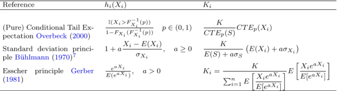
Table 1: Business Unit Driven Capital Allocation

Reference hi(Xi) Ki

(Pure) Conditional Tail Ex-pectationOverbeck(2000) I(Xi>F_Xi−1(p)) 1−F_Xi(F−1 Xi(p)) p∈(0,1) K CT Ep(S)CT Ep(Xi)

Standard deviation princi-pleBühlmann(1970)7 1 +aXi−E(Xi) σXi , a≥0 K E(S) +aσS E(Xi) +aσXi

Esscher principle Gerber

(1981) eaXi E(eaXi), a >0 Ki= K Pn i=1E XieaXi E[eaXi] E _X ieaXi E[eaXi_] ζi=h(S), i= 1, . . . , n, (34)

withhbeing a non-negative and non-decreasing function such thatE[h(S)] = 1. In this case, the states of the world to which we assign the heaviest weights are those under which the aggregate portfolio performs worst. Therefore, we call such allocationsaggregate portfolio driven allocations. The allocation rule (23) can now be rewritten as:

Ki=E[Xih(S)] +υi(K−E[Sh(S)]), i= 1, . . . , n. (35)

Hence, the capital Ki allocated to unit i is determined using a weighted expectation of the

lossXi, with higher weights attached to states of the world that involve a large aggregate loss S.

Notice that the allocation principle (35) can be reformulated as8

Ki=E(Xi) +Cov[Xi, h(S)] +υi(K−E[Sh(S)]), i= 1, . . . , n. (36)

This means that the capital allocated to the ith business unit is given by the sum of the expected lossE[Xi], a loading that depends on the covariance between the individual and

aggre-gate losses Xi and h(S), plus a term proportional to the volume of the business unit. A strong

positive correlation betweenXi andh(S), which reflects that Xi could be a substantial driver of

the aggregate lossS, produces a higher allocated capitalKi.

Using aggregate portfolio driven allocations might be appropriate when one wants to inves-tigate each individual portfolio’s contribution to the aggregate loss of the entire company. In other words, the company wishes to evaluate the subportfolio performances, for example, the returns on the allocated capitals, in the presence of the other subportfolios. This can provide rel-evant information to the company within which it can further be used to evaluate either business expansions or reductions.

Defining the volumes υi by υi =

E[Xih(S)]

E[Sh(S)] , i= 1, . . . , n. (37) PluggingEquation 37intoEquation 35we have:

8

This follows from the fact thatCov(Xi, h(S)) =E(Xih(S))−E(Xi)E(h(S))solving forE(Xih(S))we end

(24)

Ki=E[Xih(S)] + E[Xih(S)] E[Sh(S)](K−E[Sh(S)]) =E[Xih(S)] +K [Xih(S)] E[Sh(S)]−E[Xih(S)] = E[Xih(S)]E[Sh(S)] +KE[Xih(S)]−E[Xih(S)]E[Sh(S)] E[Sh(S)] .

Simplifying this last expression we end up with a proportional allocation rule:

Ki = K

E[Sh(S)]E[Xih(S)]. (38) Using the proportional allocation principle shown inEquation 38and choosing some structure forh(S)one can be allowed to construct several ways for allocatingK. For instance let us consider a particular choice forh(S)to beh(S) =S−E(S)this yields to the covariance allocation principle introduced insection 5by means of determining the expression for bothE[Xih(S)]andE[Sh(S)]

and then plug them intoEquation 38as it is shown below.

6.2.1 Covariance allocation principle

This subsection is intended to derive theCovariance allocation principle from the general setting presented in the previous section by setting h(S) = S −E(S) and using the philosophy of the plug-in principle.

Settingh(S) =S−E(S)the aim is to determine E[Xih(S)] andE[Sh(S)].

ForE[Xih(S)] the way to go is:

E[Xih(S)] =E[XiS−E(S)]

=E[XiS−XiE(S)]

=E(XiS)−E(Xi)E(S)

=Cov(Xi, S).

ForE[Sh(S)]to be explicitly found we proceed as follows:

E[Sh(S)] =E[S(S−E(S))] =E[S2−SE(S)] =E(S2)−E(S)E(S) =E(S2)−[E(S)]2 =V ar(S).

Once we have the expressions forE[Xih(S)]andE[Sh(S)]we can now plug them into Equa-tion 38in order to have the expression for allocating capitalK among the different business units

(25)

(Xi withi= 1, . . . , n) based on the Aggregate Portfolio Driven idea. So the allocation principle

has the form:

Ki = K

V ar[S]Cov(Xi, S), i= 1, . . . , n. (39) Precisely this is exactly the expression shown in Equation 15 from this fact one can notice that Covariance Principle is a special case of the Aggregate Portfolio Driven Allocation when choosingh(S) =S−E(S).

6.2.2 Overbeck allocation principles

Within this subsection we provide an explicit expression for the Aggregate Portfolio Driven Al-location principle based onOverbeck(2000). We call Overbeck Type I allocation principle to the principle obtained by setting h(S) = 1 +aS−_σE(S)

S , a ≥ 0. And we will call Overbeck Type II

allocation principle to that when usingh(S) = ₁₋1_pI(S > F_S−1(p)), withp∈(0,1).

As in the previous sections we now proceed to find an explicit expression for Ki by setting h(S) = 1 +aS−_σE(S) S , a≥0. ForE[Xih(S)] we have: E[Xih(S)] =E Xi 1 +aS−E(S) σS =E XiσS+aXi−aXiE(S) σS = 1 σS E[XiσS+aXi−aXiE(S)] =E(Xi) + a σS E(XiS)− a σS E(Xi)E(S) =E(Xi) + a σS [E(XiS)−E(Xi)E(S)] =E(Xi) + a σS Cov(Xi, S).

Working a little on E[Sh(S)] we find:

E[Sh(S)] =E S+aS(S−E(S)) σS =E(S) + a σS E[S(S−S(S))] =E(S) + a σS E S2−SE(S) =E(S) + a σS EE(S2)−E(S)E(S) =E(S) + a σS σ_S2 =E(S) +aσS.

(26)

Applying the plug-in principle and substituting the respective expressions ofE[Xih(S)] and E[Sh(S)] into the general framework presented in Equation 38 we get the allocation principle we’ve just calledOverbeck Type I allocation principle whose form is:

Ki = K E(S) +aσS E(Xi) + a σS Cov(Xi, S) . (40)

Overbeck Type II allocation principle is determined by lettingh(S)be ₁₋1_pI(S > F_S−1(p))with p∈(0,1): E[Xih(S)] = 1 1−pE[Xi|I(S > F −1 S (p))] E[Sh(S)] = 1 1−pE[S|I(S > F −1 S (p))] =CT Ep(S).

Therefore, Ki could be written as: Ki=

K CT Ep(S)

E[Xi|I(S > F_S−1(p))]. (41)

Note this principle is exactly the same one presented in Equation 14insubsection 5.2 6.2.3 Wang allocation principle

Let us considerh(S) = _Ee_[aS_eaS_]witha >0, we can construct an allocation principle based onWang

(2007) and give an expression forKi. In order to achieve our goal the procedure is similar to the

ones used in previous sections.

Once we consider h(S) = _Ee_[_eaSaS_], the expression forE[Xih(S)]is found in the following way:

E[Xih(S)] =E Sh(S) = e aS E[eaS_] = 1 E(eaS₎E(Xie aS₎ = E(Xie aS₎ E(eaS₎ .

(27)

Then E[Sh(S)]is: E[Sh(S)] =E Xih(S) = eaS E[eaS_] = E(Se aS₎ E(eaS₎ .

Therefore, the allocation of the exogenously given aggregate capital K tonpartsK1, . . . , Kn

corresponding to the different business units can be carried out using:

Ki = K

E(SeaS₎E(Xie

aS₎_. ₍₄₂₎

6.2.4 Tsanaka allocation principle

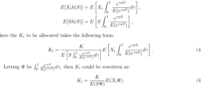
If we let R₀1_Ee₍_eγaSγaS₎ beh(S)witha >0, then this leads us to theTsanakas (2009) principle.

Expressions for constructing the Ki are as follow:

E[Xih(S)] =E Xi Z 1 0 eγaS E(eγaS₎dγ , E[Sh(S)] =E S Z 1 0 eγaS E(eγaS₎ ,

where theKi to be allocated takes the following form:

Ki = K E h SR₀1 _Ee₍_eγaSγaS₎dγ iE Xi Z 1 0 eγaS E(eγaS₎dγ . (43)

Letting ΨbeR₀1_E₍e_eγaSγaS₎dγ, thenKi could be rewritten as: Ki =

K

E(SΨ)E(XiΨ). (44)

Table 2 summarizes the Aggregate Portfolio Driven Allocations by providing expressions for

Ki.

7 Numerical Examples

Previously we introduced some well-known capital allocation principles, now we give the practical examples of these approaches and their impact on amounts of allocated capital. For this purpose we usePublic data risk no. 1 and Public data risk no. 2 from Bolancé et al.(2012), these data consist of 1000 and 400 observed loss amounts for categories 1 and 2, respectively.

Let us consider these data as operative losses in a banking environment. For Public data risk no. 1 to have some sense in this context we consider it as bank transfer mistakes which means

(28)

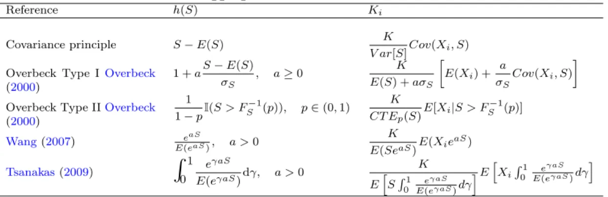
Table 2: Aggregate Portfolio Driven Allocations

Reference h(S) Ki

Covariance principle S−E(S) K

V ar[S]Cov(Xi, S) Overbeck Type IOverbeck

(2000) 1 +aS−E(S) σS , a≥0 K E(S) +aσS E(Xi) + a σS Cov(Xi, S)

Overbeck Type IIOverbeck

(2000) 1 1−pI(S > F −1 S (p)), p∈(0,1) K CT Ep(S)E[Xi|S > F −1 S (p)] Wang(2007) eaS E(eaS₎, a >0 K E(SeaS₎E(Xie aS₎ Tsanakas(2009)

R

1 0 eγaS E(eγaS₎dγ, a >0 K EhSR1 0 eγaS E(eγaS₎dγ iE h Xi R1 0 eγaS E(eγaS₎dγ i

that a bank teller transfers more money than the required to a client’s bank account andPublic data risk no. 2 is to be considered as fraudulent transactions, for instance, a client loses her credit card and another person uses it, if the bank’s client reports this situation to bank then the non-authorized use of the credit card will charge some losses to bank.

In this section we quantify individual capital requirements based on risk measures over each operative losses. Given an exogenous amount of total capital,Kcalculated as the empirical Value at Risk at 99% of the aggregate loss (VaR99(S)), the goal is allocating to each loss source an

optimal portion of this capital and comparing three well-known allocation principles: Haircut, Covariance and Overbeck type II allocation principles, all of them belonging to the proportional allocations, note that both Covariance and Overbeck type II allocation principles belong to the Aggregate portfolio allocation principle described in subsection 6.2.

The reason why we decide to use aggregate portfolio allocations is knowing the overall portfolio performance taking into account the dependence structure, meanwhile, on the other hand, we choose using Haircut allocation principle in order to make comparisons against a stand-alone risk measure which does leave out the dependence structure of the risk factors.

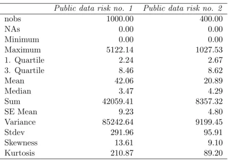
Some descriptive insights are provided inTable 3where one eye-catching fact is the difference in the number of observations in each vector of losses,Public data risk no. 1 has 1000 observations and Public data risk no. 2 has 400 which represents a drawback for the configuration of the allocation principles where all of them implicitly assume identical length for vector of losses, we overcome this inconvenient by using two different re-sampling techniques: bootstrapping and an uniformly pairwise random extraction. Another important characteristic of these data is the strong non-normality suggested by the skewness and the kurtosis coefficients, also this data show a strong right asymmetry since the mean is larger than the median for both vectors.

The numerical exercises presented below consists of two cases: the first one where the depen-dence structure is removed by the simulation procedure and in the second one a strong dependepen-dence structure between individual losses is artificially created. The aim of it is checking the perfor-mance of the allocations principles when two extreme situations might happen.

7.1 Case I: Lack of dependence structure

In this subsection, we assess the performance of allocation principles we are interested in when losses exhibit a low degree of linear dependence, this means that the correlation coefficient between

(29)

Table 3: Descriptive statistics for numerical example data Public data risk no. 1 Public data risk no. 2

nobs 1000.00 400.00 NAs 0.00 0.00 Minimum 0.00 0.00 Maximum 5122.14 1027.53 1. Quartile 2.24 2.67 3. Quartile 8.46 8.62 Mean 42.06 20.89 Median 3.47 4.29 Sum 42059.41 8357.32 SE Mean 9.23 4.80 Variance 85242.64 9199.45 Stdev 291.96 95.91 Skewness 13.61 9.10 Kurtosis 210.87 89.20

the losses is close enough to zero.

LetXandY be vectors consisting of 1000 and 400 observations on individual losses, moreover Public data risk no. 1 is now denoted byXandPublic data risk no. 2 is denoted byY. Recalling the fact that all the allocation principles presented in this thesis require the vectors to have the same length, neverthelessX andY have not that same length, this situation might be the more common one in practice, to overcome this drawback and compute the allocation principles we proceed as:9

1. Draw 1000 observations from X and 400 fromY using re-sampling with replacement and obtainX1 andY1. 2. Generate x∗₁ =P1000 i=1 X1,i and y ∗ 1 = P400 i=1Y1,i.

3. Repeat steps 1) and 2) 10000 times to obtain two vectors of equal lengths: X∗andY∗with

X∗={x∗_i}10000 i=1 and Y

∗ ₌_{_y∗ i}10000i=1 .

Once we have X∗ and Y∗ having the same length we can now compute the allocations based on the principles previously discussed.

Summarizing we generate for both vectors of losses 10000 replications of size 1000 and 400 for Public data risk no. 1 and forPublic data risk no. 2, respectively in order to obtain two vectors of length 10000 over which we can apply the allocation principle we are interested in. In thei−th

iteration we sum up all the re-sampled points to get the i−th element of each vector and we repeat this procedure 10000 times asimoves from 1 to 10000. This way the non-identical length problem of the vectors is overcome. Now we have to allocate a total amount of exogenous capital

(30)

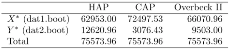
Table 4: Case I. Capital allocation based on different principles

HAP CAP Overbeck II

X∗ (dat1.boot) 62953.00 72497.53 66070.96

Y∗ (dat2.boot) 12620.96 3076.43 9503.00

Total 75573.96 75573.96 75573.96

which we estimate using an empirical VaR99(S), this means, the aggregate capital is chosen to

be the empirical Value at Risk of the aggregate loss. Note that we now have two risk sources and 10 000 observations associated to each risk source.

An aggregate capital amount of 50 416.7310 monetary units would be enough for facing the total loss for this particular sample comprised by X and Y (Public data risk no. 1 and Public data risk no. 2, respectively). Nevertheless, in order to guarantee a coverage even when large deviations might occur we use the empirical VaR99(S) =75 573.96 that ensures 99% coverage of

potential losses and this is why we set the exogenous capital to be this value. Aggregate capital to be allocated is 75 573.96 monetary units.

Table 4shows the allocated capital to each vector of losses based on different capital allocation principles, these results show the amount of capital to be set aside for each risk source. Note that Haircut allocation principle (HAP) boils down to a simple proportion when there is not any dependence structure (in a linear sense) between the losses, this happens when the correlation coefficient between X∗ and Y∗ is close to zero and in this particular case such correlation is

≈0.00014, therefore results obtained from HAP will be identical to those obtained using:

Ki = K Pn

i=1Xi

Xi, (45)

recalling the fact thatPn

i=1Xi =S, this “simple proportional” allocation principle (SPA) reduces

to (K/S)Xi. When K = 1and multiplying the result by 100 gives us the percentage ofXi as a

portion of the aggregate lossS as it is shown inTable 5.

According toTable 3 the losses seem to be non-normal, therefore both Haircut and Overbeck type II allocations are computed using the normal and the t-student distribution, for the t-student we used several degrees of freedom and results do not differ from those ones reported when using a normal distribution, so in Table 4only normal results are reported.

For we to assess how well the allocations fit, we now calculate the proportions of capital to be set aside instead of the amount of capital, we reach this goal by choosingK = 1 and the new results are reported inTable 5.

As it was expected, the Haircut allocation principle is a good choice since it does not take into account the dependence structure and since the correlation betweenX∗ andY∗is almost zero the best choice for this case is usingEquation 45as the allocation principle, because its results are the a good enough approximation for HAP and its calculation is enormously simplified, furthermore it does not rely on any distributional assumption. Table 5shows how the approximation to HAP using Equation 45performs compared to HAP results.

10

(31)

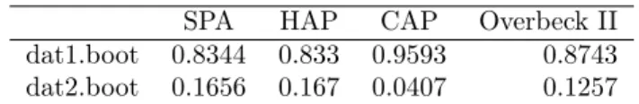
Table 5: Case I. Proportions of capital allocation based on different principles

SPA HAP CAP Overbeck II

dat1.boot 0.8344 0.833 0.9593 0.8743

dat2.boot 0.1656 0.167 0.0407 0.1257

In Table 5there is an additional column: SPA which is the approximation to the HAP when correlation tends to zero, we present this information in order to compare the proportions based on each principle. We can see that HAP is identical to SPA, nevertheless the Covariance allocation principle overestimates the contribution of the first vector and underestimates the second one in a stronger way than Overbeck II does. In a rough sense we can see that in absence of correlation between losses, the estimates of the Covariance allocation principle are more biased than those of Overbeck II.

Clearly in this part of the exercise we conclude that Covariance allocation principle performs the worst compared to the other two principles.

In the next section we introduce a strong dependence structure in order to assess the perfor-mance of the allocations which account for correlation among losses.

7.2 Case II: Strong dependence structure

This section can be seen as the counterpart of the previous one as now we go to the other extreme case where a strong dependence framework is involved.

In order to create two vectors of losses strongly correlated we base the sampling scheme on quantiles-based extractions, this means for each probability pi with i = 1, . . . ,10000, which is

common for both vectorsX and Y, recall thatX is the label for Public data risk no. 1 andY is the label for Public data risk no. 2, we take the value located at quantile given by F_X−1(pi) and F_Y−1(pi), eachpi was randomly drawn from aU(0,1), to make this point clear, we go through the

following steps:11

1. Draw randomly 10000 values from aU(0,1)for probabilities such thatp1 is one realization

ofU(0,1),p2 is another, and so on until p10000.

2. GenerateW andZ such that both are vectors of dimension10000×1 holdingF_X−1(pi) and F_Y−1(pi).

3. ConstructingW andZ this way guarantees that when we have a small value forW we also have a small value for Z and when we have a large for oneW we also have a large one for

Z. We storeW andZ into a matrix M of dimension 10000×2 so thatW andZ are now matched (pairwise).

4. Resample row-wise with replacement from M and draw 10000 pairs of observations, sum them colwise and get m1 which is a 1×2 vector, repeat this step 10000 times in order to

getmi withi= 1, . . . ,10000.

(32)

5. The data set we are going to work with is the matrixM∗ consisting of the colwise concate-nation ofmi withi= 1, . . . ,10000. M∗ should look like:

M∗=    m1,1 m1,2 .. . ... m10000,1 m10000,2   

6. We call the first column of M∗ as X0 and the second one is called Y0 where X0 is the resampled observations of the transfer mistakes (Public data risk no. 1) and Y0 is the resampled associated to the fraudulent transactions (Public data risk no. 2). Here the apostrophe does not mean transpose, it is just a way to nameXandY in order to distinguish them from the originalsX and Y.

Given that we suffer from different lengths for vectors of losses, we base this part of the exercise on a resampling technique using a uniform distribution as described above, this consists of generating 10000 random numbers from a uniform distribution, U(0,1), then we use this numbers to extract the empirical quantiles from each vectors, this way we obtain two vector of length 10000 with a strong dependence structure since each time we draw a “small” value from the first vector we also get a “small” value from the second one, the same happens with “big” values, this is because we are using the 10000 uniform number as index for the inverse distribution function to retrieve those numbers.

The correlation coefficient enrolled in this case is≈0.8875, this is the correlation betweenX0

and Y0, which is the “strong” dependence structure giving name to this section.

Following the same idea from the previous section, we consider the total capital to be allocated as exogenously determined and taken as given, so we consider this capital to be the empirical Value at Risk at 99% which is 628 724.6 monetary units.

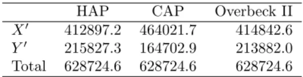
Table 6: Case II. Capital allocation based on different principles

HAP CAP Overbeck II

X0 412897.2 464021.7 414842.6

Y0 215827.3 164702.9 213882.0

Total 628724.6 628724.6 628724.6

Table 6 presents the total capital and the amounts to be allocated to each business units. Note that the first business unit, called X0 is again the riskiest one, so more capital is allocated to it. One important point, when linear dependence between these two business unit becomes higher, is that all allocation principles are very close to each other, we were aware of this fact for both CAP and Overbeck II since they takes into account the dependence structure. Looking at the Haircut allocation principle (HAP) we can see that when correlation between losses is close to one then its results quietly differ from those obtained withEquation 45, it is clearly seen since now risks are dependent each other and this is the key reason why allocations based on (the approximation to HAP) surely leads us to misleading allocations. Note that approximation provided byEquation 45, when correlation is high, becomes biased.

(33)

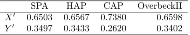
Table 7: Case II. Proportions of capital allocation based on different principles

SPA HAP CAP OverbeckII

X0 0.6503 0.6567 0.7380 0.6598

Y0 0.3497 0.3433 0.2620 0.3402

In terms of proportions, Table 7 gives a picture of how the principles distribute the total capital between the business units. The first column represents the results using Equation 45, this would be the allocation if correlation between risk sources were zero, in this case the optimal distribution of the total capital should be 65.03% allocated to the first business line (bank transfer mistakes) and 34.97% to the loss caused by fraudulent transactions. Since correlation between risk sources is 0.8910, then allocation based onEquation 45 is biased, so principles that includes the linear dependence in its calculations are needed.

In spite of the fact that HAP is based on the idea of measuring stand-alone losses using a VaR (normal VaR in this case) it performs well enough even if the correlation is high, but one has to have in mind that VaR is not a coherent risk measure so in this case it is better off using a coherent risk measure for capital allocation, from this point we can choose either Covariance allocation principle or Overbeck type II allocation principle, but in practice HAP and CAP results are not so different.

We perform a set of simulations in order to find evidence of differences among these three allocation principles when varying the correlations and running thousands of random drawings.

8 A simulation study: Assessing the

correlation effect

This section is intended to examine how sensible the allocation principles under study are when changing the linear dependence between the losses. The aim of this section is to answer, through a simulation study, the following question: How much does the allocated capital based on each principle differ when changing the correlation between the losses? In order to answer this question we consider two cases which are explained below.

The simulation study consists of drawing 100 random number from a multivariate normal distribution for two business lines with vector of means µand covariance matrix Σ for different correlation coefficients: 0, 0.1, 0.2, 0.3, 0.4, 0.5, 0.6, 0.7, 0.8, 0.9 and 1, where we can see the linear relationship goes from non-relationship at all until a perfect correlation. We apply the three capital allocation principles to these losses, and we repeat this step 1000 times, then we report the mean value of the allocations over theses 1000 results.

8.1 Case I: Risk sources with same mean and variance

In this case we consider both business lines are equally risky (in terms of variances) and also they have the same mean:12

12

(34)

µ= 42.05941 42.05941 ,

and the variance-covariance matrix takes the form:13 Σ = 94442.09 σ1,2 σ2,1 94442.09 ,

where σ1,2 = σ2,1 and it is such that we can obtain the following correlation coefficients: ρ= 0,0.1,0.2,0.3,0.4,0.5,0.6,0.7,0.8,0.9and 1.

Within this case we have two business lines with equal variances and equal means, the only difference in each replication of the simulation is the covariance (correlation) so that we can disentangle the “correlation effect” for each allocation based on the different principles which are the target of this study.

The reason why we set both, the means and the variances to be the same for both business lines, is that we expect the allocated capital to be one half in expected value for each vector, so this is a rough method to look into the robustness of each allocation principle when only the correlation is allowed to change.

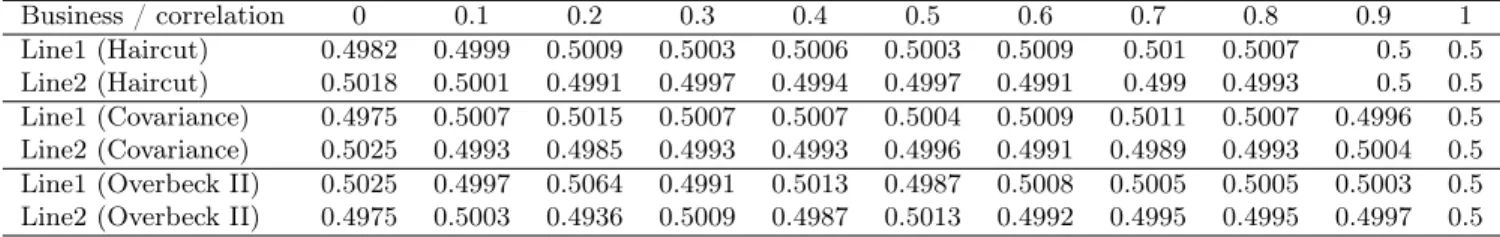
Table 8: Simulation results Case I.

Business / correlation 0 0.1 0.2 0.3 0.4 0.5 0.6 0.7 0.8 0.9 1 Line1 (Haircut) 0.4982 0.4999 0.5009 0.5003 0.5006 0.5003 0.5009 0.501 0.5007 0.5 0.5

Line2 (Haircut) 0.5018 0.5001 0.4991 0.4997 0.4994 0.4997 0.4991 0.499 0.4993 0.5 0.5

Line1 (Covariance) 0.4975 0.5007 0.5015 0.5007 0.5007 0.5004 0.5009 0.5011 0.5007 0.4996 0.5

Line2 (Covariance) 0.5025 0.4993 0.4985 0.4993 0.4993 0.4996 0.4991 0.4989 0.4993 0.5004 0.5

Line1 (Overbeck II) 0.5025 0.4997 0.5064 0.4991 0.5013 0.4987 0.5008 0.5005 0.5005 0.5003 0.5

Line2 (Overbeck II) 0.4975 0.5003 0.4936 0.5009 0.4987 0.5013 0.4992 0.4995 0.4995 0.4997 0.5

From Table 8 the main conclusion is that the linear relationship between the losses does not play any important role for the allocation principles to be good enough and whose results are almost identical, this is true (based on the simulation study) if and only if the vector of losses are characterized by the same mean and variance. This result leads us to think that there is not reason to choose one or other principle, under these circumstances (identical mean and variance) any principle gives almost the same answer.

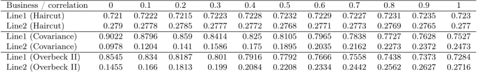
8.2 Case II: Risk sources with same mean but different variances

The second case under study in the simulation is keeping the means equal for both business lines and allowing different variances for them, and again we study the effect of correlations on the estimation of the allocated capital using the three principles which are the scope of this thesis.

The vector of means is the same as that used in the previous section and the covariance matrix now is: