S yed Z u b a ir
S ubm itted for th e Degree of D octor of Philosophy
from the University of Surrey
UNIVERSITY OF
SURREY
Centre for Vision, Speech and Signal Processing Faculty of Engineering and Physical Sciences
University of Surrey Guildford, Surrey GU2 7XH, U.K.
M arch 2014 © Syed Zubair 2014
P ro Q u e s t N u m be r: U621695
All rights reserved
INFO RM ATION TO ALL USERS
The quality of this reproduction is dependent on the quality of the copy submitted.
in the unlikely event that the author did not send a complete manuscript and there are missing pages, these will be noted. Also, if material had to be removed,
a note will indicate the deletion.
uest
P roQ uest U621695
Published by ProQuest LLC (2019). Copyright of the Dissertation is held by the Author.
Ail Rights Reserved.
This work is protected against unauthorized copying under Title 17, United States Code Microform Edition © ProQuest LLC.
ProQuest LLC
789 East Eisenhower Parkway P.O. Box 1346
Signal classification is widely applied in science and engineering such as in audio and visual signal processing. The performance of a typical classification system depends highly on the features (used to represent a signal in a lower dimensional space) and the classification algorithms (used to determine the category of the signal based on the features). Recent developments show th at dictionary learning based sparse representa tion techniques have the potential to offer improved performance over the conventional techniques for feature extraction, such as mel frequency cepstrum coefficient (MFCC) and classifier design, such as support vector machine (SVM). In this thesis, we fo cus on dictionary learning based methods for signal classification and address several challenges as explained below.
First we study the potential of using dictionary learning algorithms such as K-SVD for sparse feature extraction obtained by Orthogonal Matching Pursuit (OMP). Specifi cally, we have proposed the use of pooling and sampling techniques in audio domain to unify the dimension of feature vectors, and to improve computational efficiency. The proposed algorithm is also shown to have advantages for noisy signal classification. Most dictionary learning algorithms have been developed for vector/m atrix form of data. Our second contribution is to extend dictionary learning algorithms for high dimensional tensor data and use them to design classifiers. Different from existing tensor dictionary learning methods, we introduce various constraints on the dictionary learning process such as structured sparsity constraints on the core tensor and discrim inative constraints on the dictionaries based on the data-spread information measured by Fisher criterion. Such constraints facilitate the design of discriminative classifiers based on reconstruction error and further improve the overall performance even with reduced amount of training data.
Recently, structured block sparsity in vector/m atrix based dictionary learning method has been shown to outperform signal classification in terms of non-block sparse recon struction error. In our third contribution, we extend the concept of structured-block sparsity to tensors by providing underlying dictionaries with block structure. We de velop an algorithm for structured block-sparse tensor representation and perform clas sification based upon the block sparse tensor reconstruction error. Our algorithm shows improved performance over its m atrix based counter-parts and comparable performance with our previous tensor based method.
Our dictionary learning based classification methods are applied on audio and image data for various application scenarios such as speech and music discrimination, speaker identification, digit and face recognition. The experimental results confirm the advan tage of the proposed algorithms over several state-of-the-art baseline algorithms.
K ey w ords: Dictionary Learning, Sparse Coding, Tensor factorization and Decompo sition, Audio Classification, Machine Learning, Block Sparsity, Classification, Speaker
Recognition, Digit Recognition, Face Recognition.
Email: [email protected]
First of all, I show my humble gratitude to God who kept me persistent inspite of all odds, from Him we came and to Him we will return.
I also thank my supervisor. Dr. Wenwu Wang, who helped me to get to this stage of my work and guided me through different stages of my study.
My affection goes to my mother for her prayers, to my wife for her patience during the time of difficulties, and my loving emotions to my cheerful children who have always been the source of refreshing my mood during the stressful work of my PhD.
At the end, I acknowledge Prof. Plumbley for his earlier works in sparse representation in audio applications th at motivated me to use them in my field of research.
2.1 A three-way tensor... 26
2.2 Tensor slices and fibres, (a) Frontal, horizontal and lateral slices of a tensor, (b) Columns, rows and tubes of a tensor... 27
2.3 A rank-1 third-order tensor, Y = a o b o c... 28
2.4 PARAFAC decomposition of a third-order tensor. ... 30
2.5 A three-way TUCKER model. ... 32
3.1 Block diagram of the proposed audio signal classification system... 43
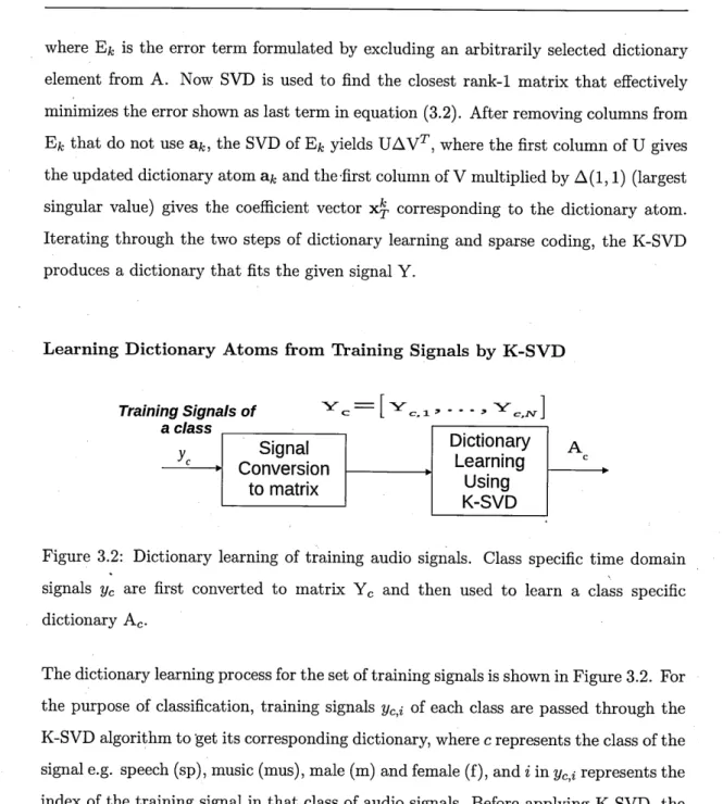
3.2 Dictionary learning of training audio signals... 45
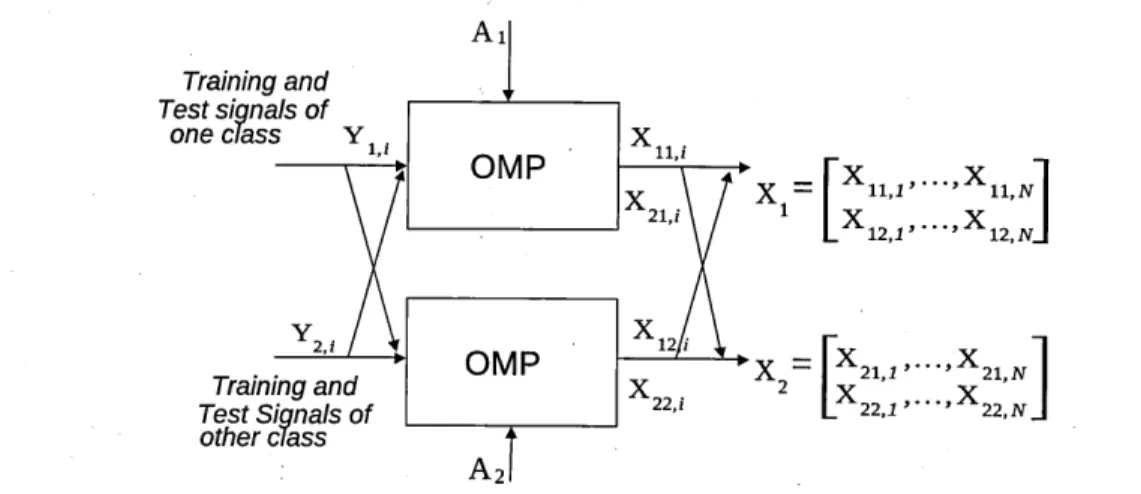
3.3 Extraction of sparse coefficients using OMP... 47
3.4 Max/average pooling of training sparse coefficient m atrix... 49
3.5 Sampling of training sparse coefficient matrix Xcd,i... 49
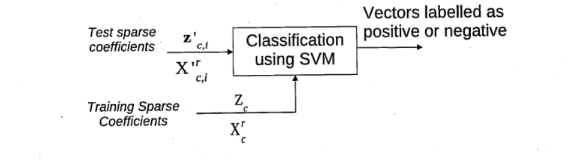
3.6 Sparse coefficients based audio signal classification using SVM... 50
3.7 Speech music classification for noisy testing d ata ... 54
3.8 Female-male speech classification for noisy testing and clean training data. 55 3.9 Speech music classification with noisy training and testing d ata... 56
3.10 Female-male speech classification with noisy training and testing data. . 57
3.11 Audio classification based on variable dictionary size... 58
3.12 Gender classification with linear and non-linear SVM. ... 59
4.1 Convergence curve of the GT-G algorithm over 100 trials... 82
4.2 Convergence curves of the GT-D algorithm... 83
4.3 Classification performance for the identification of 5 speakers... 85
4.4 Effect of the core tensor sparsity oii classification performance for digit recognition. ... 88
4.5 Classification performance for digit recognition. . ... 89 vii
viii List o f Figures
4.6 Comparison of the classification accuracy of the GT-D and TALS algo rithm s... 90 5.1 Block sparse structure of a third-order core tensor X ... 98 5.2 Face recognition rates of BT-OMP with varying block sparsity...106 5.3 Classification rates of different algorithms for a different number of train
ing examples... 107 5.4 Effect of block mode sparsity on digit recognition...108 5.5 Comparison of digit recognition performance between BT-OMP and GT-G. 108
3.1 Speaker identification performance using non-linear SVM... 59 3.2 Speaker identification performance using linear SVM... 60 3.3 Classification performances for the identification of 5 speakers using
Dic-Classifier. ... 61 4.1 Confusion matrix for the identification of 5 speakers using GT-D algorithm. 86 4.2 Confusion matrix for digit recognition using GT-D algorithm... 91 5.1 Confusion matrix for digit recognition using BT-OMP algorithm... 109
Journal A rticles
S. Zubair, F. Yan and W. Wang, “Dictionary Learning Based Sparse Coefficients for Audio Classification with Max and Average Pooling” , Digital Signal Processing (Else vier), vol. 23, pp. 960-970, 2013.
S.Zubair and W. Wang, “ Discriminative Tensor Dictionary Learning with Block-Sparse Tucker Decomposition ” , IEEE Transactions on Neural Networks . (to be submitted) S. Zubair and W. Wang, “ Dictionary Learning Algorithms for Signal Classification ” ,
Digital Signal Processing, A Review, (Elsevier), (to be submitted) Conference Papers
S. Zubair, W. Wang and J. A. Chambers, “ Discriminative Tensor Dictionaries and Sparsity for speaker Identification” , in Proc. of 4th Joint Workshop on Hands-free Speech Communication and Microphone Arrays, Nancy, France, May 12-14, 2014. (Ac cepted)
S. Zubair and W. Wang, “Tensor Dictionary Learning with Sparse Tucker Decomposi tion” , m Proc. 18th International Conference on Digital Signal Processing (DSP 2013),
Santorini, Greece, July 1-3, 2013.
S. Zubair, W. Dai, and W. Wang, “Sparseness Constrained Tensor Factorization Al gorithm for Dictionary Learning over High-Dimensional Space” , in Proc. 9th IM A International Conference on Mathematics in Signal Processing (IMA 2012), Birming ham, UK, 17-20 December, 2012.
S. Zubair and W. Wang, “Audio Classification Based on Sparse Coefficients,” in Proc. IEEE Sensor Signal Processing for Defence (SSPD 2011), London, UK, Sept 28-29,
2011.
List o f Figures vi
List o f Tables viii
List o f P u b lication s xi
1 Introduction 1
1.1 Dictionary Learning and Sparse C o d i n g ... . 3
1.2 Tensor Dictionary Learning for High-dimensional D a t a ... 5
1.3 Block Dictionary for Tensor Block S p a r s i t y ... 6
1.4 C o n trib u tio n s... 6
1.5 Thesis Outline ... 7
2 Background and L iterature Survey 9 2.1 Signal C la ssificatio n ... 9
2.2 Sparse Representation and Dictionary L e a rn in g ... 12
2.3 Dictionary Learning in Classification Applications ... 16
2.3.1 Classification Based Upon Sparse Coefficients ... 16
2.3.2 Classification Based Upon Sparse Reconstruction E r r o r ... 20
2.3.3 Learning a Classifier W ithin a Dictionary Learning Algorithm . . 23
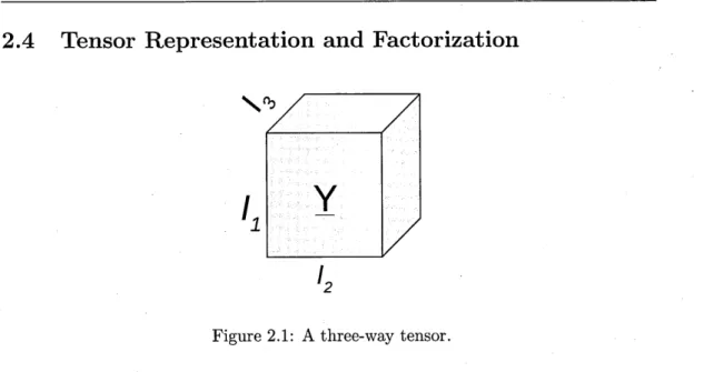
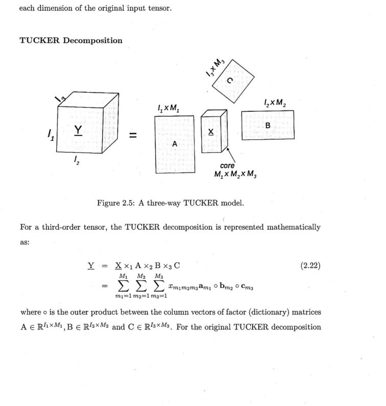
2.4 Tensor Representation and Factorization ... 26
2.4.1 Tensor Preliminaries and Notations ... 27
2.4.2 Tensor Factorization and D ecom position... 29
2.4.3 Tensor Decomposition for Classification A pplications... 35
2.5 S u m m a r y ... 37 xiii
xiv , Contents
3 D iction ary Learning B ased A udio C lassification 39
3.1 Introd uctio n ... 39
3.2 The Proposed Audio Signal Classification S y ste m ... 43
3.2.1 Dictionary Learning of Training S ig n a ls ... 43
3.2.2 Sparse Coding ... 46
3.2.3 Pooling / Sampling of Coefficients M a tr i x ... 48
3.2.4 Signal Classification by S V M ... 50
3.2.5 Extension to Multi-class Audio C lassification ... 51
3.3 Experim ents... ... 51
3.3.1 D a ta s e ts... 51
3.3.2 S e t u p ... 52
3.3.3 Results ... 53
3.3.4 Multi-class Classification... 58
3.3.5 Classification with Linear S V M ... 59
3.3.6 Comparison with DicClassifier ... 60
3.3.7 Further D iscu ssio n... 61
3.4 S u m m a r y ... 63
4 D iscrim inative Tensor D iction ary Learning for Signal C lassification 65 4.1 Introd uctio n ... 65
4.1.1 Prior W o r k ... 67
4.1.2 Motivations and Contributions . ... 68
4.1.3 Chapter O u t l i n e ... 70
4.2 Problem Formulation and Optimization C riterio n ... 70
4.3 Tensor OMP ... 73
4.4 Proposed Method: G ra d T e n so r... 75
4.4.1 General Dictionaries ( G T - G ) ... 75
4.4.2 Discriminative D ic tio n a rie s ... 77
4.5 Experiments and R esu lts... . 81
4.5.1 Simulation Study on Convergence ... 82
4.5.2 Signal C la ssificatio n ... 84
5 Tensor D iction aries w ith B lock Structure 93
5.1 Introd uctio n... 93
5.2 Classification Based on S p arsity ... 95.
5.3 Matrix Based Block Dictionary and Block Sparsity for Classification . . 95
5.4 Block Dictionary and Sparsity for T e n s o rs ... 97
5.5 M e th o d o lo g y ... 98
5.5.1 Block D ic tio n a rie s ... 98
5.5.2 Block Sparse Core T e n s o r ... 100
5.6 Experimental R esu lts... 104
5.6.1 Face R eco gn ition ... 104
5.6.2 Digit Recognition... 107
5.7 S u m m a r y ... 110
6 C onclusion and Future W ork 111 6.1 C onclusions... I l l 6.2 Future Work ...112
In trod u ction
Signal classification is an important task in different fields of science and engineering. It helps to learn relationships and structures hidden in the data and make predictions about future unseen data. It has wide spread applications in fields as diverse as business, medical sciences, astrophysics, security and surveillance [1] .
For a classification system, two components are of major importance: (1) feature ex traction (2) learning methods. For example, raw speech data often contains redundant information. In speech recognition, before training a classifier, the raw signal is first represented in a low dimensional feature space as e.g. linear predictive coding (LPC) coefficients and mel frequency cepstrum coefficients (MFCC).
Other part of the classification system, learning algorithm, uses those features to train the system. This training process gives rise to a classifier/model which defines decision boundaries for each class of signals. Inspired by human neural systems, one such learn ing algorithm is the Neural Network (NN) which emulates human neurological system to categorise a signal into its relevant class. Other examples include Decision Trees (DT) [2], Support Vector Machines (SVM) [2] and Gaussian Mixture Models (GMM) [3]. All of these algorithms are different in their utility, computational complexity, performance errors and training models. Recent developments in the field of sparse representation have given rise to dictionary learning algorithms which share a common theme of learn-from-data with the traditional learning algorithms. These algorithms
Chapter 1. Introduction
learn a classifier model from signal features. Hence a feature extraction part along with the classifier makes a complete classification system.
Depending upon the type of training data, learning methods can be divided into three categories:
• Supervised Learning • Unsupervised Learning • Semi-supervised Learning
In supervised learning, the classification model is trained by data with known label information while in case of unsupervised version, the label of the training data is unknown. However in some cases, in addition to the labelled training data, some of the data is available without label information. In this case, the learning method is known as semi-supervised.
One of the well-known unsupervised learning algorithms is K-means th at is used to learn the set of descriptive vectors These descriptive vectors constitute a codebook th a t is used to represent the input signals. In this way, a large number of input samples are represented by only one vector of the codebook with which they have the smallest distance (e.g. Euclidean distance). Though this performs a high compression of the input sample space, it lacks the more accurate representation as the input signal may be a combination of many codebook vectors and the representation of a signal by a single vector may introduce errors. This under-representation of a signal gives rise to incomplete features and thus makes it unsuitable for signal classification. This issue is addressed by the Bag of Features (BoF) model [4] th at converts an input signal into an unordered collection of local features, quantizes them into discrete features using K-means learned codebook, and then computes a compact histogram representation in terms of codebook vectors. Recent work in classification [5] shows that BoF based on sparse coding outperforms the traditional BoF model based on K-means and vector quantization particularly for image classification. This may be because of relatively coarse representation of signals in terms of K-means learned codebook as compared to sparse codes which are based on dictionary learning techniques. This motivates the use
of dictionary learning algorithms for generating sparse features th a t can be used for signal classification.
1.1
D ictio n a ry L earning and Sparse C od in g
In recent years, parametrized waveforms termed as atoms, are being used to represent signals. A collection of those atoms constitute a dictionary th at can be used to represent a signal y as:
y = A x (1.1)
where A is a dictionary matrix and x is a coefficient vector whose elements are used to linearly combine the dictionary atoms to synthesize y. Equation (1.1) can further be
represented as: '
y = Y^Xiai
(1.2)i
where represents a dictionary atom and Xi is the coefficient corresponding to In this representation, if a large number of coefficients are zero, then the representation of the signal y is considered as sparse.
Depending upon the dictionary type, a signal can be represented in terms of either pre-defined basis such as Fourier, chirplets, wavelets or the one th a t is learned from the signal. Although pre-defined dictionaries are flexible for the approximation of different types of signals, there is no guarantee th at such basis will provide best signal representation. Instead, learned dictionaries were shown to have better performance compared to pre-defined dictionaries for speech [6] and image [7] reconstruction. This may be because they are more tuned to the input signal structures.
Learned dictionaries, particularly over-complete ones where dictionary size is greater than the signal dimension, have been used for the sparse representation of signals [8]. The sparse coefficients succinctly represent the input signals by selecting those dictio nary atoms which have high contribution towards signal representation. For example in de-noising or enhancement, the sparse coefficients representing noise are different
Chapter 1. Introduction
from the one representing actual information in the signal, hence discarding the noise coefficients enhances the signal quality. This resulted in the development and deploy ment of dictionary learning based algorithms in diverse fields such as source separation
[9], coding [6], signal de-noising [7], and content analysis [10].
For signal classification, dictionary learning based algorithms have been used for audio [11], image [12] and gene classification [13]. These methods have either outperformed or showed at least comparable performances for classification as compared to the tra ditional machine learning approaches in their respective fields. This may be due to the different sparse coefficients having different support for different types (classes) of signals. The discriminative characteristics of sparse features stimulate their employ ability in classification applications. These sparse coefficients require the dictionaries containing information peculiar to a class. Hence we learn class-specific dictionaries to generate class-specific sparse coefficients. In Chapter 3, we use sparse coefficients for audio classification. When a large number of these audio signals are converted to sparse features on a frame-by-frame basis, it also poses computational complexities in training and testing phases of a classifier. Hence there is a need for a method th at could efficiently summarize the large number of sparse feature vectors per sample into a smaller number without compromising the classification performance.
Inspired by these motivations, in Chapter 3, we use dictionary learning algorithms to obtain class-specific dictionaries and introduce different variations in extracting the class-specific sparse coefficients by various pooling methods [14]. The pooling tech niques also help in selecting the most relevant dictionary atoms for sparse representation th a t boost up the overall classification performance.
The dictionary learning algorithms for signal classification are normally based on one dimensional data, called vectors. In many applications such as images and videos, the original data is available in the form of two or three dimensional (tensors) form which if converted to a vector may cause deformation of the original signal structure. Work in [15] shows th at this deformation of signal structure in matrix based learning methods make them inferior to tensor (high dimensional data) based methods in signal representation. Hence, it is highly desirable to develop algorithms that could learn
dictionaries without distorting the original multi-dimensional structure of the data. This leads to the tensor dictionary learning problem as in [16].
1.2
T ensor D ictio n a ry L earning for H ig h -d im en sio n a l D a ta
Unlike two dimensional data such as matrix, higher dimensional data is often rep resented as tensor which is formed by combining low dimensional data models (e.g. matrices) along a specific dimension. A typical example of 3-dimensional tensor is formed by stacking matrices one after the other along the third dimension.
Each dimension of the tensor contains important information which can be captured by decomposing them into its constituent factors. These factors are usually smaller in size and helps to compress the tensor data along-with capturing salient information. One such method is suggested by Tucker [16] which decomposes a tensor into its factor dictionaries and a core tensor. This core tensor coupled with the dictionaries establishes the latent relationship between different dimensions of the original tensor.
TUCKER dictionary learning algorithms have evolved through different variations in learning factor dictionaries and the core tensor. Some methods apply non-negative constraints to obtain non-negative factors [17] while others enforce sparsity on the factors along with the non-negative constraints [18].
These tensor dictionary learning methods have been used in wide applications such as computer vision, data mining and face recognition. In classification applications, the TUCKER decomposition method is used to find out either the core tensor which acts as features for input data [17] or its dictionaries th a t can be used to build up classifiers [19]. In the former case, the non-negativity as well as sparsity constraints have been applied to the dictionaries and the core tensor. However, in the latter case, only non-negative constraints have been applied as in [19]. In our work, sparsity is also applied in the second case and its effect on the classification performances is studied, as detailed in Chapter 4.
The sparsity normally applied in the TUCKER decomposition is usually unstructured where non-zero elements are scattered in the dictionaries and in the core tensor
ar-Chapter 1. Introduction
bitrarily. This configuration is useful in many applications. However, recent works in structured sparse representation for vectors show better classification accuracies as compared to non-structured one [20]. Hence there is a potential th at the classification performances could be improved if structured sparsity is employed in tensors. Thus in Chapter 4, we investigate the application of structured sparsity (block sparsity) on the core tensor of the TUCKER model to build up classifiers for tensor data.
1.3
B lo ck D ic tio n a r y for Tensor B lo ck S p arsity
Recent developments suggest th at the classification can be performed by exploiting the block sparse structure during signal reconstruction [21]. This method is based upon vector/m atrix data where a signal is classified based upon block sparse reconstruction error as opposed to non-block traditional sparse reconstruction error. In Chapter 5, we extend this concept to tensors and develop an algorithm that introduces structured block sparsity in the core tensor and the classification is also performed based upon block sparse reconstruction error. However, this requires underlying dictionary with block structure where atoms inside a block are more correlated with one another as compared to the atoms across multiple blocks. Hence we also devise a method to form block dictionaries where each block represents a sub-space of a particular class of signals.
1.4
C o n trib u tio n s
Inspired from the above mentioned motivations, we have made following contributions towards the scholastic investigation of these issues:
1. Since the classification process involves feature extraction as well as the clas sifier training, we first use dictionary learning algorithm to learn class-specific dictionaries which are then used to extract class-specific sparse features of audio signals. The sparse features obtained are then summarized to a single sparse feature vector per signal by applying pooling techniques before feeding them to a
classifier. The pooled sparse features are compared with the other conventional audio features. It is shown th a t the sparse features show high and consistent classification performance under the varying levels of additive noise.
2. We develop a new dictionary learning algorithm for multidimensional tensor data which factorizes the data block into its smaller factors with structured-sparsity (block sparsity) constraints on one of its factors (core tensor) as opposed to non structured sparsity constraints. The block sparse core tensor coupled with the dictionaries is then used to build classifiers. The block sparse structures in the core tensor helps to select those dictionary atoms which are particular to a class and thus introducing discriminative capability in the classifiers.
3. The dictionary learning algorithm developed is further extended to learn discrimi native dictionaries by incorporating additional data-spread information measured by Fisher discriminant criterion in the dictionary learning process while preserv ing the block sparsity in the core tensor. This shows improved performance for the classification applications of speaker identification and digit recognition. 4. This notion of sparsity used in tensors is further extended to the structured
block sparse core tensor along with block dictionaries. Instead of finding the sparse representation in terms of dictionary atoms, sparse representations are computed in terms of blocks of the underlying dictionaries and the classification is performed in terms of block sparse reconstruction error. This block sparse representation is then used for face recognition in comparison with the state of the art vector/m atrix based block sparse representation which shows improved performance of tensor based method over its vector/m atrix counterparts.
1.5
T h esis O u tlin e
In what follows, we begin Chapter 2 by presenting the literature of dictionary learning based sparse representation techniques with the focus being placed on signal classifica tion and their extension to high dimensional tensor data. Chapter 3 shows the classifi cation of audio signals based upon sparse coefficients with different pooling techniques.
Chapter 1. Introduction
In Chapter 4, new dictionary learning methods are proposed for high dimensional data with sparsity constraint on one of its factors. Its extension with discriminative dictio nary constraints and its application for signal classification are also included. Chapter 5 presents the extension of tensor sparse representation to deal with structured block sparsity with underlying block dictionaries. Lastly, Chapter 6 concludes the thesis along with suggestions for future work.
B ackground and L iterature
Survey
A variety of algorithms have been developed in the field of signal classification including classical methods such as support vector machine (SVM), and more recent techniques based on sparse representation and dictionary learning. In this chapter, we present an overview of the dictionary learning based classification methods and their models. We also give brief account of other traditional machine learning based classification algorithms. We then present decomposition algorithms for high dimensional data, i.e. tensors, and their use in the field of signal classification.
2.1
S ign al C lassification
The foundations of the modern classification methodologies date back to the beginning of nineteenth century when Gauss and Legendre introduced the method of least squares
which is the basis of the method now known as linear regression. Regression predicts the values of a test sample, while classification predicts the category in which a test sample lies. For example, to find the actual grade of a student in a class, regression can be applied, while to find the category of a speaker whether it is male or female, classification can be used. For this qualitative prediction, Fisher introduced linear discriminant analysis (LDA) in 1936 [1] by taking into account the spread of the data.
10 Chapter 2. Background and Literature Survey
The field of prediction and classification was further promoted to the next stage by the authors who proposed logistic regression (LR) [1] in 1940. As compared to the LDA, this method may work well if the output category is more dichotomous such as pass/fail, yes/no, healthy/ill [22]. In 1970, more generalized linear methods were introduced encompassing all the previous linear and logistic regression methods. All of these methods were proposed under the notion of linear models partly because of the prohibitive computational complexity for non-linear models at th at time.
In 1980, the advancement in computing technology facilitated the solution to non linear problems with a reasonable computational complexity. This shifted the focus of researchers from linear models to the development of non-linear models. In mid 1980s, classification and regression trees were introduced by Breiman et al. [23]. In 1986, Hastie and Tibshirani coined the term generalized additive models for a class of non-linear extensions to generalized linear models [2]. This embarked a series of developments in the machine learning and classification methods th at resulted in highly sophisticated linear/ non-linear techniques.
In a classification paradigm, the main quest is to find the category of an object with which it matches the most. For a linear classifier W G a classification problem can be represented mathematically as:
labeliy) — argm ax | z = [z i,... ,zl]^ '■= W y} (2.1) where y is a test signal, z is a label vector obtained by linear transformation of y over W, and T is the transpose of a vector.
The formation of a classifier requires the availability of some training data th at is used to build up a model of the category also termed as class. At times, the label information about the samples of the training data is not known. Depending upon the label information of the training data, the classification approach can be grouped as supervised., semi-supervised or unsupervised [22] as discussed in Chapter 1. In this thesis, we will discuss mainly the supervised classification approach.
Many supervised algorithms have been proposed to build up class models and define class boundaries for predicting the category of a test signal, such as Neural Networks
(NN) [24], Support Vector Machines (SVM) [25], Bayesian classifier [22], Gaussian Mixture Models (GMM) [3] and Markov Models (MM) [26]. The choice of a classifier can be made based upon the properties of the data. In the cases where data of different classes seem to be distinct with each another, i.e. separable, then less complex or linear classifier is preferred. However, the exact preference for the selection of a classifier can only be made after proper evaluation in the form of classification experiments [2]. Here we discuss two notable machine learning methods th at are extensively being used nowadays, namely, NN and SVM.
Inspired by the learning and activation mechanism of human biological neurons, NN tries to emulate th at mechanism with orders of magnitude less complex as compared to the human brain. For example, a human brain is made up of 85 billion neurons [27] while the current state-of-the-art NN’s have a maximum complexity of 1.73 billion neurons simulated recently by using about 83000 processors of supercomputers [28]. A simple neuron is constituted of inputs connected to a node which computes the output for incoming weighted input values. Hence a neural network is defined in terms of the algorithm th at calculates the weights, a network topology th at describes the number of neurons as well as the number of layers and manner in which they are connected and a transfer function th a t transforms the incoming values into an output value. Input features are applied to NN which are scaled by the weights and fed to a transfer function th at calculates the output value. A predefined threshold value specifies the category of the output value. However, with the increasing number of neurons and the layers, learning of the neural network parameters becomes very complex.
Another state-of-the-art algorithm, SVM, separates the data points into groups by finding a linear boundary between them, called a hyperplane. This hyperplane separates the data of two linearly separable classes in such a way th a t the d ata points closest to the hyperplane on its both sides are at maximum distance from the hyperplane. This involves the search of Maximum Margin Hyperplane (MMH) th at creates the maximum separation between the two classes. The data points from each class which are closest to the hyperplane are called Support Vectors (SV). For non-linearly separable data, some points of the data may fall on the incorrect side of the margin. In this case, a cost value is applied to all those points that fall on the incorrect side and then the algorithm
12 Chapter 2. Background and Literature Survey
attem pts to minimize th at cost. Another way of coping with this problem of non-linear separability is to use kernel-trick by mapping the problem into a higher dimensional space [29]. This mapping may convert the non-linear relationship into linear one and helps in classifying non-linearly separable data. A dot product of incoming test feature vector with the weights defining the hyperplanes decides the category of the data. In this way, traditional machine learning algorithms are used for signal classification.
2.2
S parse R ep re sen ta tio n and D ictio n a ry L earning
For a physical process, the data captured by sensors may contain redundancy due to the fact th at multiple versions of the sensor data come from the same process and hence are potentially correlated. The sampling process of the sensors is often dense and cannot reject the irrelevant information. The relevant information essential for human perception is of low dimensionality as compared to the recorded data. This curse of
dimensionality has a direct effect on the complexity of the classification algorithms. One of the earlier methods for dealing with the dimensionality issue is Principal Com ponent Analysis (PCA) [30]. PCA reduces the dimensionality by analysing the spread of the data and summarizing the correlated data into lower dimensional uncorrelated components. In some cases, the underlying causes for data generation are not located in the ensemble of data, rather they lie within different subspaces. Independent Compo nent Analysis (ICA) [31] is used to find out different sources in the production of data by analysing the higher order statistical characteristics of the data and by minimizing the mutual information between the observed signals.
Studies reveal th at human visual cortex reduces a high dimensional retinal image to a low dimensional space defined by the receptive fields of a small number of active neurons. This hypothesis triggered research in the area of sparse representation. In 1997, Olshausen and Field [32] devised method for sparse representation of the input data based upon dictionary learning and provided evidence suggesting th at the primary visual area VI in the human cortex follows a sparse coding model. If Y G is an input signal and is decomposed into a dictionary matrix A G R A *^ and a coefficient
matrix X G then the dictionary learning objective function can be formulated as:
rninQ = m m \ \ Y - A X \ \ j r - \ - X a F A { A ) X ^ F x { X ) (2.2) where Fa and F x are the regularizers for dictionary A and coefficient matrix X, respec
tively, and Xa and Xx are the penalty parameters for the regularizers. These regularizers assign certain characteristics to the dictionary and the coefficient matrix. In case of Ol shausen and Field’s work, the specific structure is only applied to the coefficient m atrix which makes each coefficient column vector sparse, hence with the sparsity constraints,
(2.2) becomes
m ina = min|| Y - A X ||J .+ A „ F x ( X ) (2.3) where f% (X ) =
II
ilo and Xj is a column vector of the coefficient m atrix X. Hence (2.3) becomesh
minC? = m i n ^ || y* - Axi ||| +A^ || Xi ||o (2.4)
A , A . A X i _
1 = 1
where || • ||o is called the £q norm and it counts the number of non-zero values in
a vector x, is the penalty th at keeps balance between the sparsity of x and the signal reconstruction error. The complexity of finding the sparest solution of y with
£q norm is NP-hard [33], hence a number of sub-optimal methods have been proposed for finding sparse representation. Those methods can be grouped as greedy methods, convex optimization based methods or local optimization based techniques. Amongst the greedy approaches, the simplest one is Matching Pursuit (MP) [34], which calculates the sparse coefficients of the input signal based upon the inner product of the residual error with the dictionary atoms. The atom which has the highest correlation with the residual error is then found and its corresponding coefficient is updated. To get a more accurate representation. Orthogonal Matching Pursuit (OMP) [35] updates the sparse coefficients by orthogonal projection of the input signal vector on all selected atoms. However, due to the least squares calculation step, OMP is relatively more demanding in terms of computational time and memory requirements. A faster approach in greedy pursuit is gradient pursuit (GP) [36] which speeds up the costly orthogonal projection step by using gradient optimization techniques.
14 Chapter 2. Background and Literature Survey
Convex optimization based sparse representation methods include Basis Pursuit (BP) [37] and Regression Shrinkage and Selection (LASSO) [38]. These methods relax the NP-hard £q norm calculation with £i norm based convex approximation and then use linear or non-linear convex optimization to obtain the solutions. Another method based upon non-convex local optimization technique is Focal Under-determined System Solver (FOCUSS) [39] which performs better than other greedy based method in the case when the atoms of dictionary are highly correlated. However, it has high computational requirement. These methods facilitate the representation of an input signal vector as a linear combination of a small number of dictionary atoms corresponding to the support of Xj. This requires the design of an over-complete dictionary th at provides an underlying subspace for sparse representation. By over-complete, we mean th at the number of atoms K in the dictionary is greater than the signal dimensionality Ii.
The problem of learning a dictionary from data is not trivial and has attracted a great deal of research attention in this field. Normally, dictionary learning algorithms are executed as a two-step process; dictionary update and sparse coding. Most of the dic tionary learning methods only differ in the way each step is performed. One class of the dictionary learning algorithms is based on the probabilistic framework [32] [40] [8] where the dictionary is sought by maximizing the likelihood function. In [32], Olshausen and Field proposed a dictionary learning algorithm based upon the maximum likeli hood learning with an assumption of sparsity promoting the distribution of the sparse coefficients as a-priori such as Laplace distribution. This assumption on the sparse coefficients makes the overall probabilistic inference complex and computationally in tensive. Following similar probabilistic approach, Kreutz-Delgado et al. [8] proposed a maximum a-posteriori probability (MAP) based learning method which replaces the likelihood function in [32] with a posterior probability and seeks for its maximization in order to learn the dictionary with sparse codes. In this case, the sparse coding is performed by FOCUSS [39] method. The Method of Optimal Directions (MOD) [40] formulates the dictionary learning problem as a least squares problem and gives a closed form expression for its computation. In sparse coding step, it uses OMP [41] for the calculation of sparse coefficients. Unlike previous methods, MOD calculates the whole dictionary and the whole sparse coefficients matrix simultaneously in their
corresponding update steps. In the majorization minimization (MajM) method [6], the actual objective function is substituted with a surrogate function th a t minimizes the objective using majorization optimization. This method computes the dictionary and the sparse codes more efficiently as compared to the other probabilistic methods. In this case, the sparse coding stage is performed by using iterative thresholding algorithm [42].
Another type of dictionary learning algorithms, known as K-SVD [7], is based on K- means clustering approach which minimizes the objective function by finding the sin gular value decomposition of the training data. This algorithm uses OMP for the calculation of coefficients in the sparse coding step. This method also calculates the dictionary and the coefficients alternatively. However, different from the other methods, in K-SVD, both the sparse coefficients and the dictionary atom are updated simulta neously in the dictionary update step.
In all these algorithms, the alternating steps of dictionary update and sparse coding are performed on the whole training data, hence their complexity increases with increase in the number of input samples. An online algorithm th a t works on real-time d ata is proposed in [43] where the two steps are performed by using the subset of the training data. In each new iteration, the subset is augmented with new training d ata and the alternating steps are run with th at new data. The results calculated in the previous step are used to initialize the new step. In this way, the dictionary and the sparse coefficients are calculated until the whole data is consumed.
Due to the adaptability of the dictionaries for different types of data and their ability to represent those data sparsely, dictionary learning methods have been used in wide areas of engineering applications such as source separation, computer vision and image processing. Since information extraction is the basis of classification, dictionary learning techniques have also been applied for classification. Research in the field of signal classification is largely driven in two directions: (1) Feature Extraction (2) Classifier Model. Hence the role of dictionary learning algorithms has also been investigated in theses two directions. In addition to that, some researchers have also introduced the learning of a stand-alone classifier in a dictionary learning algorithm [44] in the sense
16 Chapter 2. Background and Literature Survey
th a t a classifier is learned as a separate output of the algorithm.
A typical way of the application of dictionary learning algorithms for classification requires the learning of dictionaries for each class [45] [46]. These class-specific dictio naries represent the internal details of the signals from one class while rejecting the features from the other, hence each class-specific dictionary is believed to represent the corresponding class signals sparsely as compared to the other class dictionaries. In this way, the sparse coefficients thus obtained have the ability to show discrimina tive information about each class and can be used as features for classification. These class-specific dictionaries also represent the corresponding class signals with least re construction error, hence this uniqueness in the reconstruction error is another way for finding the label of a test signal based upon sparse representation. In the next section, we further discuss different ways of signal classification under the framework of dictionary learning algorithms based sparse representation.
2.3
D ic tio n a r y L earning iij C lassification A p p lica tio n s
In the framework of dictionary learning and sparse coding, signal classification is per formed mainly in three different ways, as discussed next.
2.3.1 C lassification B a sed U p o n Sparse C oefficients
In this way, with a given underlying dictionary, sparse codes are computed which act as class features and are supplied to any classifier used in the conventional machine learn ing methods. In this model, there are three factors which differentiate the classification systems based upon sparse coefficients. These are:
• Methodology th at is used for the extraction of sparse codes. • Type of dictionary and the dictionary learning technique. • Type of a classifier th at is used for classification.
In one of the pioneering works for the use of sparse representations in audio applications, Plumbley et al. [47] suggested the use of sparse representation for polyphonic music which triggered wide use of this concept in various fields of signal classification in general and for audio applications in particular.
As discussed before, one of the earliest methods for extracting sparse coefficients was proposed by Mallat and Zhang [34] known as matching pursuit (MP), hence the sparse coefficients derived by this method were also termed as MP sparse features. In [48], Chu et al. suggested the use of these sparse features for the classification of environmental sounds in comparison with MFCC features which are widely used in audio processing applications. The MP sparse features are extracted with an underlying pre-defined Fourier dictionary. A Gaussian mixture model (GMM) is used as a classifier to inves tigate the performance of MP features over conventional MFCC features. The results suggest th at MP features offer better performance over the MFCC features.
The same concept of MP features is further extended in [49] for a dataset of envi ronmental sound th at is different from those used in [48]. The MP sparse features extracted in this work are further decomposed into two separate matrices, one for the temporal and other for the spectral features, by using non-negative m atrix decompo sition method proposed in [50]. The dictionary used here for the extraction of MP features is based upon Cabor function. These extracted features are supplied to linear discriminant analysis (LDA) classifier for audio classification.
The benefits of the sparse features over the conventional audio features were further explored in other areas of audio classification problems. In [51], Scholler and Purwins studied the use of these MP sparse features for drum classification in comparison with MFCC features. However, unlike previous methods which use a pre-defined fixed dic tionary for the extraction of sparse features, a learned dictionary is used which is based on the optimization method proposed in [52]. The classification method employed here is based upon Random Forests (RF) proposed in [53].
The above systems use MP method for the extraction of sparse features which show good performance for audio classification applications. However, with the increase in the number of training samples, the number of sparse feature vectors used to train the
18 Chapter 2. Background and Literature Survey
classifier such as SVM also increases. This introduces computational burden for training classifiers. In addition, due to the increased computational complexity introduced when dealing with a large number of sparse feature vectors derived from the audio frames, such problem is also likely to occur during the test phase. Hence, in Chapter 3, we use an improved version of MP, OMP, for the extraction of sparse features along with the pooling techniques th at summarize a data sample consisting of many sparse vectors into a single sparse feature vector which reduces the computational cost in the training / testing phase. Moreover, the pooled sparse features also show promising results over conventional MFCC features. A similar approach has also been taken in [54] where OMP and K-SVD are used for contour detection in image segmentation problem. The gradient of the image is used to detect its contours which are supplied to the K-SVD to generate gradient sparse coefficients with OMP based upon the learned dictionary. The pooling technique suggested in our work, as demonstrated in Chapter 3, along with the OMP features is further extended to a multi-layer OMP algorithm in [55]. The algorithm is designed to take into account all the modalities of input signal such as images in which each patch has its own local properties. For this purpose. Bo et al. in [55] propose a multilayer m ultipath version of the OMP algorithm. The algorithm starts with small raw patches of the image, and then learns its mutually incoherent dictionary on those small patches along with sparse coding step using OMP. The resulting sparse codes are spatially pooled to form bigger patches followed by the normalization which are fed as input to the next layer. The same process of mutually incoherent dictionary learning and sparse coding is performed on the output of the previous layer and same operations of pooling and normalization are also repeated. In this way, a hierarchical m ultipath sparse coding is performed which gives rise to sparse representation of the input image at the final stage. This sparse representation is then supplied to a linear SVM for signal classification.
Signal classification requires th a t the features used should have a discriminating nature. This discriminant behaviour, however, is not very robust to noise and the outliers [56], and hence some inherent ability against these odds is required. Sparse representation of the signals is very powerful for reconstruction purposes and has inherent ability against noise [57]. Hence in [58], Huang and Aviyente combine the discriminative
ability of linear discriminant analysis (LDA) with the reconstruction power of sparse representation. Inspired by OMP like methods, both characteristics, discriminant as well as noise tolerance, are induced in the sparse features based upon a greedy technique. The dictionaries, however, used for this purpose are pre-defined dictionaries such as Haar wavelet and Gabor basis. The sparse representation found in this case acts as features for the SVM classifier.
In all the above methods, the OMP operates on the input vectors one after the other. Si multaneous sparse coding method (SOMP) proposed in [59] uses OMP for simultaneous coding of the input signals. SOMP finds out the sparse representation of all the input samples at once as a linear combination of a common subset of atoms. To add more discriminative capability to these SOMP based coefficients, an LDA based discriminant criterion is proposed in [60] which is applied on class-specific SOMP coefficients. W ith this discriminant sparse coding stage, dictionary is learned based upon K-SVD [7] in an alternating minimization fashion. The discriminative sparse coefficients thus obtained are then applied to a linear SVM for classification.
In [61], again SOMP is used for the extraction of sparse coefficients but with a different dictionary learning algorithm, MOD. However, by exploiting the sparse structure of the signals belonging to the same class, these sparse codes are first used to divide the input samples into distinct groups and then the subset of the dictionary atoms is selected th at best represents the input samples in a group. The sparse coefficients extracted in this way are used for classification based on SVM.
In some cases, input signals are shift-invariant such as audio signal or rotational / trans lational invariant such as images. The sparse coefficients of such transform-invariant signals are better represented by their respective transform-invariant dictionaries. To address this issue, the authors in [62] propose sparse coding and shift-invariant dictio nary learning method in which input signals are reconstructed using all shifts of the dictionary atoms. They also used SVM for the classification of sparse features gener ated through such a dictionary. In case of images. Bar and Sapiro in [63] propose a hierarchical dictionary learning method for taking into account rotational, translational and scaling variations of the input images.
20 Chapter 2. Background and Literature Survey
In [64], unlike greedy algorithms, the authors use an encoder suggested in [65] that maps a signal efficiently into its sparse components. This method is known as Predic tive Sparse Decomposition (PSD). This encoder is trained on the sparse codes which are obtained during the dictionary learning process, with dictionary learned using a stochastic gradient method. The extracted sparse features are used to train SVM for music classification.
In most of the above classification schemes, sparse coefficients are obtained using class- specific dictionaries. Different from this approach, the authors in [66] build up one large dictionary for all the classes. The dictionary is learned by using an online dictionary learning algorithm [43] applied for texture classification. A positivity constraint is applied on the sparse coefficients calculated for each texture image which are used to build up histograms of each texture image. These histograms are then used for classification using nearest neighbour classifier.
Recently in [67], sparse coding has been proposed for transfer learning in which the labelled and the unlabelled data come from different distributions. In this case, sparse coding is performed in such a way th at the difference between the probability distribu tion of labelled and unlabelled data is minimized. For this purpose, a maximum mean discrepancy (MMD) metric is used to compare the distance between samples means of sparse codes for labelled and unlabelled data. An alternating dictionary learning and sparse coding optimization algorithm is proposed in which the dictionary is learned by an ^2-norm constrained least squares method while sparse coding is performed by
^i-norm regularised least squares method along with minimizing the MMD metric. The classifier used here for the classification of sparse codes is logistic regression (LR).
2 .3 .2 C la s s if ic a tio n B a s e d U p o n S p a r s e R e c o n s t r u c tio n E r r o r
In this method, the reconstruction error of a test signal based upon sparse representa tion is used to classify the signal [46]. Mathematically, a class label for the test signal y in terms of sparse representation is given as:
where x* is the optimized sparse vector th a t gives the minimum reconstruction error in above equation and A i is the dictionary of the z-th class giving the best representation for the test signal, x* is found with the help of OMP algorithm.
One of the earlier works th at used the reconstruction error for signal classification was presented in [68] for texture classification of images. In this work, a dictionary is termed as a frame and sparse codes are calculated by using Order Recursive Matching Pursuit (ORMP) [69]. The classification is performed using the sparsity based reconstruction error as in (2.5). However, to further lower the classification error, smoothing is applied on the reconstructed images before the reconstruction error is calculated.
Another approach in this category combines the reconstructive power of the learned dic tionaries with discriminative ability by introducing discrimination inducing constraints in dictionaries, as in [70]. In this work, separate dictionaries are learned for each class along-with discriminative properties. Dictionaries are made discriminative by intro ducing a softmax [70] cost function which makes a dictionary highly re-constructive for its own class but generates low energy coefficients for the other classes. The sparse coefficients are calculated using OMP and the dictionary is updated using a K-SVD like approach.
Unlike [70], Yang et al. in [71] suggest the use of a unified dictionary containing the dictionaries of all triasses. Each class specific dictionary is considered as sub-dictionary. The sub-dictionaries are learned with a constraint th a t the projection of the sparse coefficient vector of a signal over all the subspaces is zero except the subspace of its own class. Here the dictionaries are learned by the method suggested in [72] using a Lagrange dual which converts a constrained objective function into an unconstrained one by using penalty parameters. The classification is done based upon sparse repre sentation as in equation (2.5).
D ic tio n a rie s w ith sp ecial s tr u c tu r e
Following equation (2.2), the regularizer term Fa (A) defines dictionaries with special
structures. In the context of classification, this special structure normally makes the dictionary more discriminative and helps in improving the classification performance.
22 Chapter 2. Background and Literature Survey
In [12], multiple dictionaries are learned one for each class with discrimination promot ing term F^(A ). In this case. F a (A) = Q introduces incoherence among the dictionaries and is defined as:
Q = min || A J A j ||^ (2.6) if ;
where A% and A j are the dictionaries related to different classes i and j respectively and subscript F is Frobenius norm. In this work, the classification method based upon the sparse reconstruction is also somewhat different from a common approach given in (2.5). Though (2.5) gives good classification results in [70], it does not take into account the sparsity constraint on the coefficient vector. Hence, the authors use
label{y) = arg nun || y - A*x* \\l 4-y || x* jji (2.7) for signal classification which also takes into account the sparsity of the coding coeffi cients. The dictionary learning and sparse coding are performed using a variation of the learning algorithm presented in [73].
To make the dictionaries more discriminative, Fisher criterion [74] based constraint proposed in [45] is applied to the class dictionaries. In this work, two discriminative fidelity terms are added to the objective function of the dictionary learning algorithm. One of the terms ensures th at the signal of a class is best reconstructed with its own dictionary in terms of the £ 2 norm and less accurately represented by other dictionaries. This is done by minimizing the signal reconstruction error with the ensemble of class- specific dictionaries and the dictionary of its own class and also by minimizing the signal reconstruction energy with its own class dictionary. These three quantities constitute one fidelity term. The other term applies the Fisher criterion on each class while learning its sparse coefficients. In this way, the class-specific dictionary and the sparse coefficients both exhibit the discerning features that can improve the classification performance with the classification criterion based on (2.7). In Chapter 4, we have extended this Fisher criterion for learning the dictionaries from high dimensional tensor data.
In the dictionary learning objective function defined in [45], the first discrimination fi delity term decreases the distance between the input signal space and the space spanned
by their own class dictionaries and increases its distance from the space spanned by the dictionaries of other classes, yet the class-specific dictionaries still share some atoms which are common to all classes. To purge the dictionaries with shared atoms, Kong and Wang in [75] introduce the concept of particular dictionaries and a common dictio nary. To remove the common atoms from class-specific dictionaries, a coherence term defined in (2.6) is combined with the first discriminative fidelity term defined in [45] (as discussed in above paragraph in the context of [45]) and added as a constraint to the objective function for dictionary learning. The coherence measure also helps to find out the related atoms in the class-specific dictionaries which are combined in a dictionary called common dictionary. The classification of a test signal is performed based on the reconstruction of the signal using a class-specific dictionary augmented with the common dictionary. The label for the class-specific dictionary th a t gives the minimum reconstruction error is assigned as the label for the test signal.
A new dictionary learning technique is formulated as a graph topology selection prob lem in [76]. The data samples are considered as nodes of a graph and their pairwise relations with one another as its edges. In graph topology selection process, a graph topology is sought where the new topology edges are subset of the original topology edges and consists of K connected components. The graph is partitioned into K
-clusters and the centres of the -clusters are considered as the dictionary atoms. By applying discriminative constraints, these clusters are also made class-specific so th a t the sparse representations of signals pertaining to one class have similar structure. The cluster centre of a matching class shows high peak in the sparse representation and hence provides the label for the signal under consideration.
2.3.3 Learning a C lassifier W ith in a D ictio n a ry L earning A lg o r ith m
In this methodology, apart from learning a dictionary and sparse coefficients, the learn ing algorithm also seeks for a separate independent classifier as a separate learning output. This classifier acts as a transformation matrix to assign a label to a test signal as given in equation (2.1).
24 Chapter 2. Background and Literature Survey
which dictionary is learned jointly along-with the logistic loss function based classifier [77]. An objective function is formulated to learn the dictionary for sparse coding along with the parameters of a classifier. Since three different quantities have to be learned, i.e. a dictionary, a sparse code and the parameters of the classifier, a block coordinate descent method is used in which sparse coefficients are calculated while fixing the dictionary and the classifier parameters. In the next iteration, sparse codes are kept fixed while the dictionary and the classifier parameters are learned. The dictionary and the classifier are learned using a projected gradient method. Given a learned dictionary and a classifier, the test signal is classified by finding its supervised sparse code with a given dictionary and minimizing the cost function with the learned classifier which assigns a label to the test signal. The whole objective function is made discriminative by not only minimizing the prediction error of the test signal with the learned classifier for one class but also maximizing the error with other classes.
This joint optimization of the dictionary and the classifier not only requires many parameters to be tuned, but also suffers from the problem of local minima. In discrim inative K-SVD (DK-SVD) [78], a linear classifier is again learned with the dictionary but not in alternating minimization manner. Rather labels of the input signals and the classifier transformation matrix are augmented with the input signals and dictionary atoms column-wise in a matrix in such a way th at in the new input signal vector, the upper sub-vector represents the input signal and the lower sub-vector shows its label. The lower-submatrix of the dictionary is also augmented with the linear classifier pa rameters in the same way. Then the dictionary along with the classifier is learned by using K-SVD. The sparse coding step uses the same OMP algorithm. In this way, when the K-SVD algorithm completes its iterations, the dictionary along with a classifier is also learned. The classification is performed by finding the sparse coefficients of a test signal and then projecting them linearly on to the classifier.
Though in [77] block coordinated descent methods are used to learn the dictionary and the classifier alternatively, this method and the DK-SVD are both batch-oriented approaches and their algorithmic complexity increases with the increase in the batch size (size of the data). In [79], the authors also used the same block coordinate descent method as in [77] and the joint optimization of dictionary and the classifier is formu
lated in a way similar to DK-SVD [78], but the d ata is consumed in an online fashion. Inspired by [43], the dictionary and the classifier learning are performed in an online fashion such th a t the algorithm progressively uses the data in the form of mini batches. When the new data comes in, the dictionary and the classifier learned in the previous iteration become the initialization point for the next iteration. In this way the dictio nary and the classifier are learned until the whole data is consumed. The optimization method used in this work is stochastic gradient method which assumes th a t the input data is independent and identically distributed (i.i.d.). Since the distribution of the input data is practically unknown, hence obtaining i.i.d. samples of the input data is difficult. However, a common trick is used to obtain such i.i.d. samples by cycling over a randomly permuted training set [80].
In a Bayesian framework of dictionary learning algorithm [81] where dictionary and sparse representation are determined using Bayesian non-parametric models [82], the authors in [83] extend this concept by learning the dictionary, the sparse codes and the classifier simultaneously. The dictionary is learned based upon a Beta-Bernoulli process [84] along with the sparse codes. To make the dictionary discriminative, a logistic regression classifier is incorporated into the probabilistic learning model of the d