Mining multi-dimensional concept-drifting
data streams using Bayesian network
classifiers
Hanen Borchani
a,, Pedro Larrañaga
a, João Gama
band Concha Bielza
aaComputational Intelligence Group, Departamento de Inteligencia Artificial, Facultad de Informática,
Universidad Politécnica de Madrid, Madrid, Spain
bLIAAD-INESC Porto, Faculty of Economics, University of Porto, Porto, Portugal
Abstract. In recent years, a plethora of approaches have been proposed to deal with the increasingly challenging task of mining concept-drifting data streams. However, most of these approaches can only be applied to uni-dimensional classi-fication problems where each input instance has to be assigned to a single output class variable. The problem of mining multi-dimensional data streams, which includes multiple output class variables, is largely unexplored and only few stream-ing multi-dimensional approaches have been recently introduced. In this paper, we propose a novel adaptive method, named
Locally Adaptive-MB-MBC (LA-MB-MBC), for mining streaming multi-dimensional data. To this end, we make use of multi-dimensional Bayesian network classifiers (MBCs) as models. Basically, LA-MB-MBC monitors the concept drift over time using the average log-likelihood score and the Page-Hinkley test. Then, if a concept drift is detected, LA-MB-MBC adapts the current MBC network locally around each changed node. An experimental study carried out using synthetic multi-dimensional data streams shows the merits of the proposed method in terms of concept drift detection as well as classification performance.
1. Introduction
Nowadays, with the rapid growth of information technology, huge flows of records are generated and collected daily from a wide range of real-world applications, such as network monitoring, telecom-munications data management, social networks, information filtering, fraud detection, etc. These flows are defined as data streams. Contrary to finite stationary databases, data streams are characterized by their concept-drifting aspect [37,39], which means that the learned concepts and/or the underlying data distribution are not stable and may change over time. Moreover, data streams pose many challenges to computing systems due to limited memory resources (i.e., the stream can not be fully stored in memory), and time (i.e., the stream should be continuously processed and the learned classification model should be ready at any time to be used for prediction).
In recent years, the field of mining concept-drifting data streams has received an increasing attention and a plethora of approaches have been developed and deployed in several applications [1,5,11,15,17,
Corresponding author: Hanen Borchani, Computational Intelligence Group, Departamento de Inteligencia Artificial, Facul-tad de Informática, Universidad Politécnica de Madrid, Boadilla del Monte, 28660 Madrid, Spain. Tel.: +34 913363675; Fax: +34 913524819; E-mail: [email protected].
39]. All proposed approaches have a main objective consisting of coping with the concept drift and maintaining the classification model up-to-date along the continuous flows of data. They are usually composed of a detection method to monitor the concept drift and an adaptation method used for updating the classification model over time.
However, most of the work within this field has only been focused on mining uni-dimensional data streams where each input instance has to be assigned to a single output class variable. The problem of mining multi-dimensional data streams, where each instance has to be simultaneously associated with multiple output class variables, remains largely unexplored and only few multi-dimensional streaming methods have been introduced [23,30,33,40].
In this paper, we present a new method for mining dimensional data streams based on multi-dimensional Bayesian network classifiers (MBCs). The so-called Locally Adaptive-MB-MBC (LA-MB-MBC) extends the stationary MB-MBC algorithm [6] to tackle the concept-drifting aspect of data streams. Basically, LA-MB-MBC monitors the concept drift over time using the average log-likelihood score and the Page-Hinkley test. Then, if a concept drift is detected, L A - M B - M B C adapts the current MBC network locally around each changed node. An experimental study carried out using synthetic multi-dimensional data streams shows the merits of the proposed adaptive method in terms of concept drift detection and classification performance.
The remainder of this paper is organized as follows. Section 2 briefly defines the multi-dimensional classification problem, then introduces multi-dimensional Bayesian network classifiers. Section 3 dis-cusses the concept drift problem, and Section 4 reviews the related work on mining multi-dimensional data streams. Next, Section 5 introduces the proposed method for change detection and local MBC adap-tation. Sections 6 and 7 cover the experimental study presenting the used data, the evaluation metrics, and a discussion on the obtained results. Finally, Section 8 rounds the paper off with some conclusions and future works.
2. Background
2.1. Multi-dimensional classification
In the traditional and more popular task of uni-dimensional classification, each instance in the data set is associated with a single class variable. However, in many real-world applications, more than one class variable may be required. That is, each instance in the data set has to be associated with a set of many different class variables at the same time. An example would be classifying movies at the online internet movie database (IMDb). In this case, a given movie may be classified simultaneously into three different categories, e.g. action, crime and drama. Additional examples may include a patient suffering from multiple diseases, a text document belonging to several topics, a gene associated with multiple functional classes, etc.
Hence, the multi-dimensional classification problem can be viewed as an extension of the uni-dimensional classification problem where simultaneous prediction of a set of class variables is needed. Formally, it consists of finding a function / that predicts for each input instance given by a vector of m features x = (x\,...,xm), a vector of d class values c = (ci,...,c^), that is,
/ : QXl x ... x QXm — ^ d x ... x QCd
where Qxi and Qc3 denote the sample spaces of each feature variable Xi, for alli e {1,...,m}, and
each class variable Cj, for all j e {1,...,d}, respectively. Note that, we consider that all class and feature variables are discrete random variables such that |Qx31 and |Qc31 are greater than 1.
When |He | = 2 for all j e {1,...,d}, i.e., all class variables are binary, the multi-dimensional classification problem is known as a multi-label classification problem [25,36,42]. A multi-label classi-fication problem can be easily modeled as a multi-dimensional classiclassi-fication problem where each label corresponds to a binary class variable. However, modeling a multi-dimensional classification problem, that possibly includes non-binary class variables, as a multi-label classification problem may require a transformation over the data set to meet multi-label framework requirements.
Since our proposed method is general and can be applied to classification problems where class vari-ables are not necessarily binary, we opt to use, unless mentioned otherwise, the term multi-dimensional classification as a more general concept.
2.2. Multi-dimensional Bayesian network classifiers
A Bayesian network [22,28] over a finite set U = {X\,...,Xn}, n ^ 1, of discrete random variables
is a pair B = (Q, x). Q = (V,A) is a directed acyclic graph (DAG) whose vertices V correspond to variables Xi and whose arcs A represent conditional dependence relationships between triplets of variables. 0 is a set ofparameters such that each of its components QXi\va(Xi) = P(xi\pa(xi)) represents
the conditional probability of each possible value Xi of Xi given a set value pa(a;j) of Pa(Xj), where Pa(-Xj) denotes the set of parents of Xi (nodes directed to Xi) in Q. The set ofparameters 0 is organized in tables, referred to as conditional probability tables (CPTs). B defines a joint probability distribution over U factorized according to structure Q given by:
n
P(x\,... ,xn) = I I P(xi\pa(xi)) (1)
Two important definitions follow:
Definition 1. Two sets of variables X and Y are conditionally independent given some set of variables Z, denoted as /(X, Y|Z), iff P(X|Y, Z) = P(X|Z) for any assignment of values x, y, z of X, Y, Z, respectively, such that P(Z = z) > 0.
Definition 2. A Markov blanket of a variable X, denoted as MB(X), is a minimal set of variables with the following property: I(X,S\MB(X)) holds for every variable subset S with no variables in
MB(X) U X.
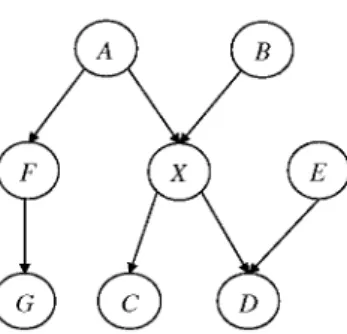
In other words, MB(X) is a minimal set of variables conditioned by which X is conditionally indepen-dent of all the remaining variables. Under the faithfulness assumption, ensuring that all the conditional independencies in the data distribution are strictly those entailed by Q, MB(X) consists of the union of the set of parents, children, and parents of children (i.e., spouses) of X [29]. For instance, as shown in Fig. 1, MB(X) = {A, B, C, D, E} which consists of the union of X parents {A, B}, its children
{C, D}, and the parent of its child node D, i.e., {E}.
A multi-dimensional Bayesian networks classifier (MBC) is a Bayesian network specially designed to deal with the emerging problem of multi-dimensional classification.
Definition 3. An MBC [38] is a Bayesian network B = (Q,x) where the structure Q = (V, A) has a restricted topology. The set of n vertices V is partitioned into two sets: Vc = {C\,..., C^}, d ^ 1, of class variables and Vx = {X\,...,Xm}, m ^ 1, of feature variables (d + m = ri). The set of arcs A is
Fig. 1. The Markov blanket of X denoted MB(X) con- Fig. 2. An example of an MBC structure. sists of the union of its parents {A, B}, its children
{C,D}, and the parent {E} of its child D.
- Ac c Vc x Vc is composed of the arcs between the class variables having a subgraph Qc = (Vc,Ac) - class subgraph -ofQ induced by Vc.
- Ax c Vx x Vx is composed of the arcs between the feature variables having a subgraph Qx = (Vx,Ax) –feature subgraph -ofQ induced by Vx.
- Acx ^ Vc x Vx is composed of the arcs from the class variables to the feature variables having a
subgraph Qcx = (V, Acx) - bridge subgraph -of Q induced by V [4].
Classification with an MBC under a 0-1 loss function is equivalent to solving the most probable explanation (MPE) problem, which consists of finding the most likely instantiation of the vector of class variables c* = (c|,...,c*d) given an evidence about the input vector of feature variables x = (x1,..., xm). Formally,
c* = (c\,...,c*i) = arg max p(C1 = c1,... ,Cd = Cd|x) (2)
ct,...,cd
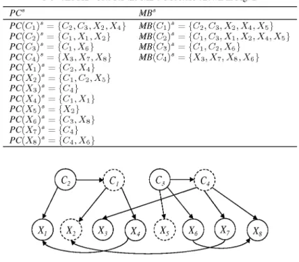
Example 1. An example of an MBC structure is shown in Fig. 2. The class subgraph Qc = {{C1,
...,C4}, Ac) such that Ac consists of the two arcs between the class variables C1, C2, and C3, the
feature subgraph Qx = {{X1,..., X8}, Ax) such that Ax contains the three arcs between the feature variables, and finally, the bridge subgraph Qcx = ({C1, • • •, C4,X1,..., X8}, Acx) such that Acx is composed of the eight arcs from the class variables to the feature variables. As an MPE problem, we have max P(c1,..., C4|x) = max P(c1\c2, c3)P(c2)P(c3)P(c4) C i , . . . , C 4 C i , . . . , C 4 • P(X1\C2, X4)P(X2\C1, C2,X5)P{X3\c4)P{X4\c1) • P(:c5)P(:c6|c3)P(:c7|c4)P(:c8|c4,:c6) 3. Concept drift
In uni-dimensional data streams, concept drift refers to the changes in the joint probability distribution
P(x, c) which is the product of the class posterior distribution P(c\x) and the feature distribution P(x).
Therefore, three types of concept drift can be distinguished [17,37]: conditional change (also known as real concept drift) if a change occurs in P(c|x); feature change (also known as virtual concept drift) if a change occurs in P(x); and dual change if changes occur in both P(c\x) and P(x).
categorized into either abrupt or gradual. An abrupt concept drift occurs at a specific time point by suddenly switching from one concept to another. On the contrary, in a gradual concept drift, a new concept is slowly introduced over an extended time period. An additional categorization is based on whether the concept drift is local or global. A concept drift is said to be local when it only occurs in some regions of the instance space (sub-spaces), and global when it occurs in the whole instance space [12].
Several additional concept drift categorizations may be found in literature such as the one proposed by Minku et al. [26] characterizing concept drifts according to different additional criteria, namely, severity (severe if no instance maintains its target class in the new concept, or intersected otherwise), frequency (periodic or non-periodic) and predictability (predictable or random). Concept drifts may be also reoccurring if previously seen concepts reappear (generally at irregular time intervals) over time, or
novelties when some new variables or some of their respective states appear or disappear over time [16].
The same definitions and categorizations of uni-dimensional concept drift can be applied in the con text of multi-dimensional data streams. In fact, the feature change involving only a change in P(x) is exactly the same; whereas, for the conditional change, we have now a vector of d class variables C = (Ci,...,Cd) instead of a single class variable C, i.e., the conditional change may occur in the dis tribution P(c|x). Moreover, as previously, the change is called dual when both feature and conditional changes occur together. Furthermore, the multi-dimensional concept drift can be also categorized into
abrupt or gradual depending on the rate of change, and into local or global depending on whether it
occurs in some regions of the instance space or in the whole instance space, respectively.
Consequently, the main differences between the uni-dimensional and the multi-dimensional concept drifts consist mainly of the changes that may occur in the distribution and the dependence relationships between the class variables, as well as the distribution and the dependence relationships between each class variable and the set of feature variables.
Besides these categorizations, and in the context of streaming multi-label classification, Read et al. [33] discuss that concept drift may also involve a change in the label cardinality, that is, a change in the average number of labels associated with each instance computed as LCard = l/N J2i=i J2j=i c\ with c- ∈ {0,1}, where N denotes the total number of instances and d the number of labels (or binary class variables).
In addition, Xioufis et al. [40] consider that a multi-label data stream contains separate multiple targets (concepts) and each concept is likely to exhibit independently its own drift pattern. This assumption allows to track the drift of each concept separately using for instance the binary relevance method [18]. In fact, binary relevance proceeds by decomposing the multi-label learning problem into d independent binary classification problems, such that each binary classification problem aims to predict a single label value. However, the main drawback of this assumption is the inability to deal with the correlations that concepts may have with each other and which may drift over time.
It is important to note that the different presented types of drift are not exhaustive and the categoriza tions discussed here are not mutually exclusive. In our case, we particularly deal with a local concept
drift in multi-dimensional data streams. Moreover, as mentioned later in Section 6.1, we consider for the
empirical study different rates for local concept drifts, i.e., either abrupt or gradual.
4. Related work
In this section, we review the existing related works. All have been developed under the streaming multi-label classification setting, and can be viewed as extension of stationary multi-label methods to concept-drifting data streams.
Qu et al. [30] propose an ensemble of improved binary relevance (MBR) taking into account the depen-dency among labels. The basic idea is to add each classified label vector as a new feature participating in the classification of the other related labels. To cope with concept drifts, Qu et al. use a dynamic clas-sifier ensemble jointly with a weighted majority voting strategy. No drift detection method is employed in MBR. In fact, the ensemble keeps a fixed number K of base classifiers, and is updated continuously over time by adding new classifiers, trained on the recent data blocks, and discarding the oldest ones. Naive Bayes, C4.5 decision tree algorithm, and support vector machines (SVM) are used as different base classifiers to test the MBR method.
Xioufis et al. [40] tackle a special problem when dealing with multi-label data streams, namely class
imbalance, i.e., the skewness in the distribution of positive and negative instances for all or some labels.
In fact, each label in the stream may have more negative than positive instances, and some labels may have much more positive instances than others. To deal with this problem, the authors propose a multiple windows classifier (MWC) that maintains two windows of fixed size for each label: one for positive instances and one for negative ones. The size Np of the positive windows is a parameter of the approach
and the size Nn of the negative windows is determined using the formula Nn = Np/r, where r is
another parameter of the approach, called distribution ratio. r has the role of balancing the distribution of positive and negative instances in the union of the two windows. The authors assume an independent concept drift for each label, and use a binary relevance method [18] with fc-nearest neighbors (fcNN) as base classifier. No drift detection method is employed in MWC. Positive and negative windows of each label are updated continuously over time by including new incoming instances and removing older ones.
Moreover, Kong and Yu [23] propose also an ensemble-based method for multi-label stream classifi-cation. The idea is to use an ensemble of multiple random decision trees [41] where tree nodes are built by means of random selected testing variables and spliting values. The so-called Streaming Multi-lAbel Random Trees (SMART) algorithm does not include a change detection method. In fact, to handle con-cept drifts in the stream, the authors simply use a fading function on each tree node to gradually reduce the influence of historical data over time. The fading function consists of assigning to each old instance with time stamp U a weight w(t) = 2~(-t~ti^x, where t is the current time, and A is a parameter of the
approach, called fading factor, indicating the speed of the fading effects. The higher the value of A, the slower the weight of each instance will decay.
Finally, Read et al. [33] present a framework for generating synthetic multi-label data streams along with a novel multi-label streaming classification ensemble method based on Hoeffding trees. Their method, named EaHTps, extends the single-label incremental Hoeffding tree (HT) classifier [10] by using a multi-label definition of entropy and by training multi-label pruned sets (PS) at each leaf node of the tree. To handle concept drifts, Read et al. use the ADWIN Bagging method [5] which consists of an online bagging method extended with an adaptive sliding window (ADWIN) as a change detector. When a concept drift is detected, the worst performing classifier of the ensemble of classifiers is replaced with a new classifier. Read et al. also introduce BRa, EaBR, EaPS, HTa methods, that extend respectively binary relevance (BR) [18], ensembles of BR (EBR) [32], ensembles of textttPS (EPS) [31], and multi-label Hoeffding trees (HT) [8] stationary methods by including ADWIN to detect the potential concept drifts.
The presented streaming multi-label methods are summarized in Table 1. Contrary to these methods, which are all based on a multi-label setting, requiring all the class variables to be binary, our proposed adaptive method has no constraints on the cardinalities of the class variables. Moreover, these methods either do not present any drift detection method (for instance, MBR [30], MWC [40] and SMART [23] approaches) or they use a drift detection method and keep updating an ensemble of classifiers over
Table 1
Summary of streaming multi-label classification methods
Reference Method Base classifier Adaptation strategy Qu et al. [30] Ensemble of improved
binary relevance (MBR)
Xioufis et al. [40] Multiple windows classifier (MWC)
Naive Bayes, C4.5, SVM fcNN Random tree Evolving ensemble. No detection
Two windows of fixed size for each label. No detection
Fading function. No detection Kong and Yu [23] Streaming multi-label
random trees (SMART)
Read et al. [33] Ensemble of multi-label Hoeffding tree Evolving ensemble.
Hoeffding trees with PS at the leaves Detection using the ADWIN algorithm
(EaHTPS), as well as BRa, EaBR, EaPS, and HTa methods
time by replacing the worst performing classifier with a new one when a drift is detected (such as EaHTps [33] using ADWIN algorithm as a change detector). In both cases, the concept drift cannot be detected locally, and the adaptation process is basically based on ensemble updating.
In our case, we only use a single model (i.e., MBC) and our proposed drift detection method performs locally: it is based on monitoring the average local log-likelihood of each node of the MBC network using the Page-Hinkley test. Being based on MBCs, our adaptive method presents also the merit of explicitly modeling the probabilistic dependence relationships among all variables through the graphical structure component.
5. Locally adaptive-MB-MBC method
Before providing more details about the proposed approach, let us introduce the following notation. Let D = {D1,D2,...,Ds,...} denote a multi-dimensional data stream that arrives over time in batches,
such that Ds = {(x(1), c( 1 )) , . . . , ( x( N s ), c( N s )) } denotes the multi-dimensional batch stream received
at step s, and containing Ns instances. For each instance in the stream, the input vector x = ( x1, . . . ,xm)
of m feature values is associated with an output vector c = ( c1, . . . ,cd) of d class values. For the sake of
simplicity, and regardless of being class or feature variable, we denote by Vi each variable in the MBC, i = 1,... ,n, such that n represents the total number of variables, i.e., n = d+m. Given an MBC learned
from Ds, denoted MBCs, and a new incoming batch stream Ds+1, the adaptive learning problem consists
of firstly detecting possible concept drifts, then, if required, updating the current MBCs, as MBCs+1, to
best fit the new distribution of Ds+1.
In what follows, we start by presenting the proposed drift detection method in Section 5.1. Next, we introduce the MBC adaptation method in Section 5.2.
5.1. Drift detection method
The objective here is to continuously process the batches of data streams and detect the local concept drift when it occurs. As mentioned before, this local concept drift can also be either abrupt or gradual. Our proposed detection method is based on the average local log-likelihood score and the Page-Hinkley test, and is applied locally, i.e., to each variable in the MBC network.
C1 C2 • C3 • C4 8 10 Block number
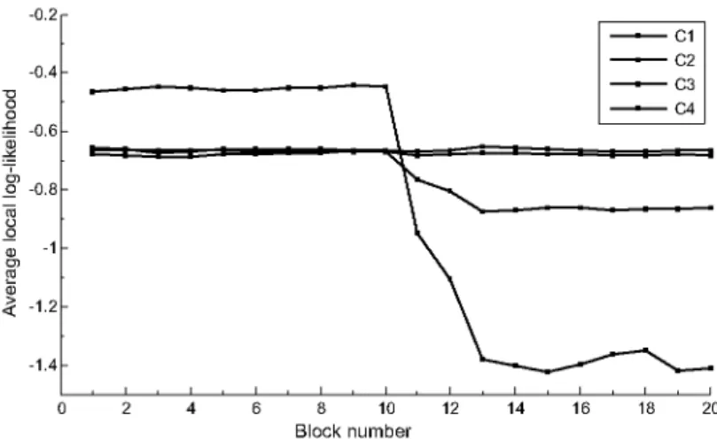
Fig. 3. The evolution of the average local log-likelihood values of four different class variables, namely C1, C2, C3, and C4. (Colours are visible in the online version of the article; http://dx.doi.org/10.3233/IDA-160804)
5.1.1. The average local log-likelihood score
The likelihood measures the probability of a data set Ds given the current multi-dimensional Bayesian
network classifier. For convenience in the calculations, the logarithm of the likelihood is usually used:
Ns n n qi Ti
LLS = log P(Ds\0s) = log I I I I P{v\ |pa(vj)' ', 6s) = 2, /_, / , log 7ijk ) Nf (3)
l=\i=\ i=\ j=\ k=\
where v\ , pa(^j) ^ are respectively the values of variable Vi and its parent set Pa(V^) in the /t h instance
in Vs. ri denotes the number of possible states of Vi, and qi denotes the number of possible
configura-tions that the parent set Pa(V^) can take. N?-k is the number of instances in Vs where variable Vi takes
its kth value and Pa(V^) takes its jt h configuration.
We consider then the average log-likelihood score in Vs, which is equal to the original log-likelihood
score LLS divided by the total number of instances Ns. This in fact will allow us to compare the
like-lihood of an MBC network based on different batch streams that may present different numbers of instances. Hence, using the maximum likelihood estimation for the parameters, 6, ijk N ijk
Nfj = Yfk=i ^tjk for every i, • • • ,n, the average log-likelihood can be expressed as follows:
n -. Hi Ti ]\TS L L = y —— y y wi7-fc log ——— ^—' NNs s ^—' ^—' J N %=\ j=\ k=\ where (4) V
Finally, since the change should be monitored on each variable, we use the average local log-likelihood of each variable Vi in the network expressed as:
u:
Ns i Qi Ti N?jk Nijk log —— ij (5) j=1 k=1Example 2. To illustrate the key idea of using the average local log-likelihood to monitor the concept drift, we plot, in Fig. 3, the evolution of the average local log-likelihood values of four different class variables, namely, C1, C2, C3, and C4. As it can be observed, the average local log-likelihood values for
C2 and C3 are stable over time, which means that there is no concept drift for both variables. However, -0.2 -0.4 -0.6 -0.8 --1.2 -1.4 0 2 4 6 2 4 6 8 20
abrupt and gradual concept drifts could be detected for variables C1 and C4, respectively, as their cor-responding average local log-likelihood values drop at block 10. In the next section, we will introduce how to detect this drift point using as input the average local log-likelihood values of each variable.
5.1.2. Change point detection
In recent years, several change detection methods have been proposed to determine the point at which the concept drift occurs. As pointed out in [16], these methods can be categorized into four groups: i) methods based on sequential analysis such as the sequential probability ratio test; ii) methods based on control charts or statistical process control; iii) methods based on monitoring distributions on two different time-windows such as the AD WIN algorithm; and iv) contextual methods such as the splice system. More details about these methods and their references can be found in [16], Section 3.2.
In this work, In order to detect the change point, we make use of the Page-Hinkley (PH) test [20,27]. The PH test is a sequential analysis technique commonly used for change detection in signal processing, and has been proven to be appropriate for detecting concept drifts in data streams [34].
In particular, we apply the PH test in order to determine whether a sequence of average local log-likelihood values of a variable Vi can be attributed to a single statistical law (null hypothesis); or it
— 1 — s demonstrates a change in the statistical law underlying these values (change point). Let lliy... ,1^,
denote the average local log-likelihood values for variavle Vi computed with Eq. (5) using the first batch stream D1 till the last received one Ds, respectively. To test the above hypothesis, the PH test considers
first a cumulative variable CUMf, defined as the cumulated difference between the obtained average local log-likelihood values and their mean till the current moment (i.e., the last batch Ds):
s
CUMf = 2_,(^h - meanjjt - 5) (6)
where mean-^ = 1 ^2h=1 11 j denotes the mean of lli,..., 11 i values, and 5 is a positive tolerance
pa-rameter corresponding to the magnitude of changes which are allowed. The maximum value MAXS of variable CUM* for t = 1 , . . . , s , is then computed:
MAXf = max iCUM\,t = 1,...,s\ (7)
Next, the PH value is computed as the difference between MAXS and CUMS:
PHf = MAXf - CUMf (8)
When this difference is greater than a given threshold A (i.e., PHf > A), the null hypothesis is rejected and the PH test alarms a change, otherwise, no change is signaled. Specifically, depending on the result of this test, two states can be distinguished:
- If PHf ^ A then there is no concept drift: the distribution of the average local log-likelihood values is stable. The new batch Ds is deemed to come from the same distribution as the previous data set
of instances.
- If PHf > A then a concept drift is considered to have occurred: the distribution of the average local log-likelihood values is drifting. The new batch Ds is deemed to come from a different distribution
than the previous data set of instances.
The threshold A is a parameter allowing to control the rate of false alarms. In general, small A values may increase the number of false alarms, whereas higher A values may lead to a fewer false alarms but may rise at the same time the risk of missing some concept drifts.
Note that, the PH test is designed here to detect decreases in the log-likelihood, since an increase in the log-likelihood score informs that the current MBC network still fits well the new data and thus no adaptation is required. In our case, each local PH test value, PHf, allows us to check if a drift occurs or not at each considered variable Vi. This in fact will locally specify where (i.e., for which set of variables) the concept drift occurs. Afterwards, the challenge is to locally update the MBC structure, i.e., update only the parts that are in conflict with the the new incoming batch stream without re-learning the whole MBC from scratch.
5.2. Local MBC adaptation
The objective here is to locally update the MBC network over time, so that if a concept drift occurs, only the changed parts in the current MBC are re-learned from the new incoming batch stream and not the whole network. This presents two main challenges: First, how to locally detect the changes, and second how to update the current MBC.
To deal with these challenges, we propose the Locally Adaptive-MB-MBC method, outlined by Algorithm 1. Given the current network MBCS, the new incoming batch stream Ds+l, and the PH test
parameters 5 and A, the local change detection firstly computes the average log-likelihood 11 i of each
variable Vi using the new incoming batch stream Ds+l (step 4), then computes the corresponding value PHl+l (step 5). Next, if this PH^+1 value is higher than A, then variable Vi is added to the set of nodes to
be changed (steps 6 to 8). Subsequently, whenever the resulting set of ChangedNodes is not empty, i.e., a drift is detected, then the UpdateMBC function, outlined by Algorithm 2, is invoked to locally update the current MBCS network (step 11); otherwise, we conclude that no drift is detected and the MBC network
is kept unchanged (step 13).
Algorithm 1 Locally Adaptive-MB-MBC
1. Input: Current MBCS, new multi-dimensional data stream Ds+1, 5, A
2. ChangedNodes = 0 3. for every variable V, do
4. Compute the average local log-likelihood l^ using Eq. (5) 5. Compute the local PH test, PH^+1
6. if PH^+ > A then
7. ChangedNodes <— ChangedNodes U {Vi} 8. end if
9. end for
10. if ChangedNodes ^ 0 then
11. MBCS+ <— UpdateMBC(ChangedNodes,MBCs,Ds+l ,PCS,MBS)
12. else
13. MBCs+l <— MBCS, i.e., no drift is detected
14. end if
15. return MBCS+
Before introducing the UpdateMBC algorithm, note that since the local log-likelihood computes the probability of each variable Vi given the set of its parents in the MBC structure, then a detected change for a variable Vi informs that the set of parents of the variable Vi has changed due to either the removal of some existing parents or the inclusion of new parents:
- The removal of an existing parent means that this parent was strongly relevant to Vi given Ds, and
becomes either weakly relevant or irrelevant to Vi given Ds+1. In other words, this parent was a
member of the parent set, or more broadly a member of the parents-children set of Vi, but with respect to Ds+1, it does not pertain to the parents-children set of Vi.
- The inclusion of a new parent means that this parent was either weakly relevant or irrelevant to Vi given Ds, and becomes strongly relevant to Vi given Ds+1. In other words, this parent was not a
member of the parents-children set of V,, but with respect to Ds+1, it should be added as a new
member of the parents-children set of Vi.
Recall that, variables are defined to be strongly relevant if they contain information about Vi not found in all other remaining variables. That is, the strongly relevant variables are the members of the Markov blanket of Vi, and thereby, all the members in the parents-children set of Vi are also strongly relevant to
Vi. On the other hand, variables are said to be weakly relevant if they are informative but redundant, i.e.,
they consist of all the variables with an undirected path to Vi which are not themselves members of the Markov blanket nor the parents-children set of Vi. Finally, variables are defined as irrelevant if they are not informative, and in this case, they consist of variables with no undirected path to Vi [2,21].
Therefore, the intuition behind UpdateMBC algorithm, is basically to firstly learn with Ds+1 the new
parents-children set of each changed node using the HITON-PC algorithm [2,3], determine the sets of its old and new adjacent nodes, and then locally update the MBC structure.
UpdateMBC is outlined by Algorithm 2. It takes as input the set of changed nodes, the current
net-work MBCS, the new incoming batch stream Ds+1, the parents-children sets of all variables PCS, and
the Markov blanket sets of all class variables MBS. For each variable Vi in the set of changed nodes, UpdateMBC initially learns from Ds+1 the new parents-children set of Vi, PC(V)s+1, using
HITON-PC algorithm (step 3). Then, it determines the set of its old adjacent nodes, i.e., {HITON-PC(Vi)s \ PC(Vi)s+1
(step 4). The variables included in this set are variables that pertained to PC(V)S but do not pertain
any-more to PC(Vi)s+1, which means that they represent the set of variables that were strongly relevant to V,
and have become either weakly relevant or irrelevant to V,. In this case, for each variable OldAdj belong-ing to this set, the arc between it and V, is removed from MBCs+1 (step 5), then, the parents-children
and Markov blanket sets are updated accordingly. Specifically, the following rules are performed: - Remove Vi from the parents-children set of OldAdj (step 6): since the arc between Vi and OldAdj
was removed, Vi does not pertain anymore to the parents-children set of OldAdj.
- If the old adjacent node OldAdj is a class variable, then update its Markov blanket MB(OldAdj)s+1
by removing from it the changed node Vi and its parents that do not belong to the parents-children set PC(OldAdj)s+1 of OldAdj (steps 7 to 9).
- If the changed node Vi is a class variable, then update its Markov blanket MB(Vi)s+1 by removing
from it the old adjacent node OldAdj and its parents that do not belong to the parents-children set of Vi, PC(Vi)s+1 (steps 10 to 12).
- Update the Markov blanket of each class variable that belongs to the parent set of Vi, without being a parent nor a child of OldAdj, by removing from it the old adjacent node OldAdj (steps 13 to 15). Subsequently, UpdateMBC determines the set of the new adjacent nodes of the changed node Vi, de-noted as 1 PC(Vi)s+1 \ PC(Vi)s (step 17). The variables included in this set are variables that belong to
PC(Vi)s+l but they were not previously in PC(V)S, which means that they represent the set of variables
that were weakly relevant or irrelevant to V, and become strongly relevant to Vi. Hence, new depen-dence relationships should be inserted between those variables and Vi verifying at each insertion that no cycles are introduced. In this case, a new arc is inserted from each new adjacent node NewAdj to
V, (step 18), then the parents-children and Markov blanket sets are updated accordingly. The following
Algorithm 2 UpdateMBC(ChangedNodes, MBCs,Ds+1, PCs, MBs) 1. Initialization: MBCS+ <— MBCS; PCS+ <— PCs;MBs+1 <— MBS 2. for every variable V, G ChangedNodes do
3. Learn PC(Vi)s+1 <— HITON-PC(Vi)
#Determine the set of the old adjacent nodes of the changed node Vi
4. for every variable OldAdj e {.PC(Vi)s \ PC(Vi)s+1 do 5. Remove the arc between OldAdj and Vi from MBCs+1
6. PC(OldAdj)s+1 <— PC(OldAdj)s+1 \ {Vi} 7. if OldAdj £ Vc then
8. MB(OldAdj)s+1 <— MB(OldAdj)s+1 \ {V, U {Pa(Vi)s+1 \ PC(OldAdj)s+1} 9. end if
10. if Vi G Vc then
11. MB(Vi)s+1 <— MB(Vi)s+1 \ {OldAdj L) {Pa(OldAdj)s+1 \PC(V,)S+1}
12. end if
13. for every class if e {Pa(Vi)s + 1 \ PC(OldAdj)s+1 do 14. MB(H)s+1 <— MB(H)s+1 \ {OldAdj}
15. end for 16. end for
#Determine the set of the new adjacent nodes of the changed node Vi
17. for every variable NewAdj e {PC(Vi)s+1 \ PC(Vi)s do 18. Insert an arc from NewAdj to Vi in MBC'S+1
19. PC(NewAdj)s+1 <— PC(NewAdj)s+1 U {Vi}
20. if NewAdj £ Vc then
21. MB(NewAdj)s+1 <— MB(NewAdj)s+1 U {Vi U Pa(Vi)s + 1}
22. end if
23. if Vi G Vb then
24. MB(Vi)s+1 <— MB(Vi)s+1 U {NewAdj U Pa(NewAdj)s+1}
25. end if
26. for every class H £ {Pa(Vi)s + 1 \ {NewAdj U PC(NewAdj)s+1} do
27. MB(H)s+1 <— MB(H)s+1 U {NewAdj}
28. end for 29. end for 30. end for
31. Learn from _DS+1 new CPTs for nodes that have got a new parent set in MBCs+1
32. return MBCS+1; PCS+1; MBs+1
- Add Vi to the parents-children set of NewAdj (step 19): since an arc was inserted between Vi and
NewAdj, Vi becomes a member of the parents-children set of NewAdj.
- If the new adjacent node NewAdj is a class variable, then update its Markov blanketMB(NewAdj)s+1
by adding to it the changed node Vi as well as its parent set Pa(Vi) (steps 20 to 22).
- If the changed node Vi is a class, then update its Markov blanket MB(Vi)s+1 by adding to it NewAdj
and its parent set Pa(NewAdj) (steps 23 to 25).
- Update the Markov blanket of each class variable that belongs to the parent set of Vi, without being a parent nor a child NewAdj, by adding to it the new adjacent node NewAdj (steps 26 to 28).
Table 2
PCs and MBs sets for the MBC structure shown in Fig. 2
PC pc(c\) pc(c2) pc(c3) pc(c4) PC(Xi)s pc(x2) pc(x3) pc(x4) pc(x6) pc(x6) pc(x7) pc(x8) {C2,C3,X2,X4} {Ci,Xi,X2} {C\,X6} {X3,X7,X8} {C2,X4} {Cl,C2, {d} { 2} {C3,Xs} {CA} {C4,X6} ,x6} MBS MB(C\) MB(C2) MB(C3) MB(C4) {C2,C3,X2,X4,X5} {C1,C3,X1,X2,X4,X6} {C1,C2,X6} {X3,X7,X8,X6}
Fig. 4. Example of an MBC structure including structural changes in comparison with the initial MBC structure in Fig. 2. Nodes C1, C4, X2, and X5, represented in dashed line, are characterized as changed nodes.
Finally, new conditional probability tables (CPTs) are learnt from Ds+1 for all the nodes that have got
a new parent set in MBCs+1 (step 31), and then the updated MBC network MBCs+1, the sets PCs+1 and MBs+1 are returned in step 32.
Note here that, all variables that belong to both PC(Vi)s and PC(Vi)s+1 of a changed node Vi do not
trigger any kind of change. In fact, these variables were strongly relevant to Vi and are still strongly
relevant to Vi, so that the dependence relationships between them and Vi remain the same. Moreover, the
order of processing the changed nodes does not affect the final result, that is, independently of the order, the updated MBC network MBCs+1 and the sets PCs+1 and MBs+1 will be the same by the end of the UpdateMBC algorithm. This is guaranteed because the identification of the old and new adjacent nodes
is performed independently for each changed node, and thereby, it is not affected by the order nor by the results of other nodes. The updating process of PC and MB sets is also ensured via simple operations such as removing or adding variables, and hence, the order of variable removal or addition will not affect the final sets.
Example 3. To illustrate the Locally Adaptive-MB-MBC algorithm, let us first reconsider the structure shown in Fig. 2 as an example of an MBCs structure learnt from a batch stream Ds using
the MB-MBC algorithm [6]. Then, let assume that we receive afterwards a new batch stream Ds+1
generated from the MBCs+1 structure shown in Fig. 4. Given both MBCs and Ds+1, the Locally
Adaptive-MB-MBC algorithm starts by computing the average log-likelihood and the PH test for each variable in MBCs. A change should be signaled for variables C1, C4, X2, and X5 by Algorithm 1,
i.e., ChangedNodes = {C1,C4,X2,X5}. Then, the MBC network should be locally updated via the
c
2) *( c,
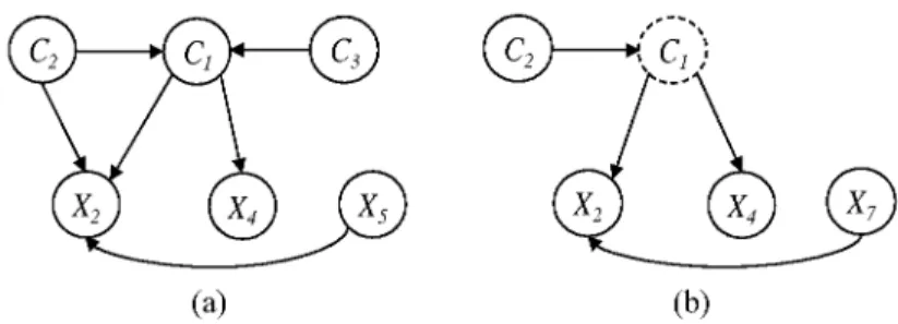
(a) (b) Fig. 5. Markov blanket of node C1 (a) before and (b) after change.
(a) (b)
Fig. 6. Markov blanket of node C4 (a) before and (b) after change.
The UpdateMBC algorithm updates the local structure around each changed node, then updates ac-cordingly the parents-children and Markov blanket sets. Note that UpdateMBC takes as input the current network MBCS, the set of ChangedNodes, the new incoming batch stream Ds+1, as well as the current
parents-children sets of all the variables PCS, and the current Markov blankets sets of all the class
vari-ables MBS, all represented in Table 2.
In what follows, we present a trace of UpdateMBC algorithm for each variable in the ChangedNodes set:
- The changed node C\ (see Fig. 4): Firstly, we determine the new parents-children set of C\ given
Ds+l using the HITON-PC algorithm (i.e., step 3 in Algorithm 2). We assume that HITON-PC de-tects the new parents-children set of C\ correctly, so we should have PC(C\)s+l = {C2,X2,X4}.
Next, we determine the set of old and new adjacent nodes for C\.
* For the old adjacent nodes, the steps 5 to 15 in Algorithm 2 would be performed. In this case, we have PC(C\)S \ PC(C\)s+l = {C3}, which means that C\ has only C3 as an old adjacent node.
Thus, we start by removing the arc between C\ and C3 (step 5); update the parents-children set of
C3 as follows: PC(Cs)s+l = PC(Cs)s+l \{C} = {XQ} (step 6); then, since C3 belongs to Vc,
we proceed by updating also the Markov blanket of C3 as follows: MB(Cs)s+1 = MB(Cs)s+1 \ {C\ U {Pa(Ci)s+1 \ PC(Cs)s+1}}. As it can be seen, we have P a ( C i )s + 1 \ PC(Cs)s+1 = {C2}, hence, C2 should be removed from the Markov blanket of C3, which results finally in: MB(C;i)s+l = MB(C;i)s+l \ {C\,C2} = {XQ} (steps 7 to 9).
Moreover, since C\ belongs to Vc, we update as well the Markov blanket of C\, i.e.,
MB(C\)s+l = MB(C\)s+l \ {C3 U {Pa(CS)S+1 \ PC(C\)S+1}} = {C2,X2,X^,Xz} (steps
10 to 12).
Finally, we update the Markov blanket set of each class parent of C\ (steps 13 to 15). In our case, we have only C2 as parent of C\, which does not pertain to PC(Cs), thus C3 should
(Cj) (Cj
{X2} \X-7j \^2) \^5 {X5 }
(a) (b) (a) (b) Fig. 7. Parents-children set of node X2 (a) before and (b) Fig. 8. Parents-children set of node X5 (a) before and (b) after change. after change.
be removed from the Markov blanket of C2, that is, MB(C2)s+l = MB(C2)s+l \ {C3} = { C1,X\,X2,X4,X5 }.
* For the new adjacent nodes, we have PC(C\)s+l \ PC(C\)S = 0. Thus, no new dependence
relationships must be added for C\.
- The changed node C4 (see Fig. 6): The first step is to determine the new parents-children set of C4 given Ds+l and using the HITON-PC algorithm. As previously, we assume that HITON-PC detects
the new parents-children set of C4 correctly, so we should have PC(C^)S~^1 = {C3,X3,Xj,Xg}.
* Next, we determine the set of old adjacent nodes, which in our case is empty, i.e, PC(C^)S \ PC(C4)s+l = 0.
* Then, the set of new adjacent nodes which is equal to PC(C^)S~^1 \ PC(C4)S = {C3}.
Conse-quently, we insert an arc from C3 to C4 (step 18), we update PC(Cs)s+l = PC(Cs)s+l U {C4} = {C4,XQ} (step 19), andMB(Cs)s+l = MB(Cs)s+llJ{C4L)Pa(C4)s+l} = {C^,XQ} (step20to 22). Similarly, update the Markov blanket set MB(C4)s+l = MB(C4)s+l U {C3 U Pa(Cs)s+1} = {Cs,Xs,Xj,Xg,XQ} (steps 23 to 25). C4 has no more parents except C3, so steps 26-28 in the UpdateMBC algorithm are not applied in this case.
- The changed node X2 (see Fig. 7): As previously, the first step is to determine the new parents-children set of X2 given Ds+l and using the HITON-PC algorithm. Assuming that HITON-PC
detects the new parents-children set of X2 correctly, we should have PC(X2)s+l = {C\,Xj}.
* Next, given that PC(X2)S = {C\,C2,X*,}, the set of old adjacent nodes is determined as PC(X2)S \ PC(X2)S+l = {C2,X5}.
For the first old adjacent node C2, we remove the arc between C2 and X2, we update
PC(C2)s+l = PC(C2)s+l \ {X2} = {C\,X\}, and we update MB(C2)s+l = MB(C2)s+l \ {X2 U {Pa(X2)s+1 \ PC(C2)s+l}}. Here X2 has two parents namely C\ and X5 (in fact X5
is not removed yet from the set of parents of X2 because we start by processing the old adja-cent variable C2), and since C\ pertains to PC(C2)s+l, the only variables to be removed from MB(C2)s+l are then X2 and X$, i.e., MB(C2)s+l = {C\,X\,X4}.
For the second old adjacent node X5, we remove the arc between X5 and X2, we update
PC(X^)s+l = PC(X§)s+l \ {X2} = 0, then update the Markov blanket set for every class
variable of X2 that does not pertain to PC(X^)s+l. In our case, X2 has only C\ as a class
par-ent (because both C2 and X5 have been already removed), so its Markov blanket is modified as follows MB(C\)s+l = MB(C\)s+l \ {X5} = {C2,X2,X^}.
* For the new adjacent nodes, we have PC(X2)s+l \ PC(X2)S = {Xj}. Thus, we insert an arc
from Xj to X2, update PC(Xj)s+1 = PC(Xj)s+1 U {X2} = {C4,X2}, then update the Markov
blanket set for every class variable of X2 that does not pertain to PC(Xj)s+l. In our case, X2
has only C\ as a class parent, which is different from Xj and not pertaining to PC(Xj), so its Markov blanket is modified as follows MB(C\)s+l = MB(C\)s+l U {Xj} = {C2,X2,X4,Xj}.
- The changed node X5 (see Fig. 8): The first step is to determine the new parents-children set of
X5 given Ds+l and using the HITON-PC algorithm. Assuming that HITON-PC detects the new parents-children set of X5 correctly, we obtain PC(X^)s+l = {C3}.
* Then, given that PC(X^)S = {X2}, we determine first the set of old adjacent nodes PC(X^)S \ PC(X^)s+l = {X2}. Since the changed variable X2 has been processed before the changed
node X5, we can see that the arc between these two variables has been already removed during the previous phase. Moreover, X5 has been already removed from PC(X2)s+l, so there is no
change for PC(X2)s+l = {C\,Xj}. X5 at this step has no class parents, so steps 13-15 in the UpdateMBC algorithm are not applied in this case.
* For the new adjacent nodes, we have PC(X5)s+l\PC(Xs)s = {C3}. Thus, we insert an arc from C3 to X5, update PC(Cs)s+l = PC(Cs)s+l U {X$} = {C4,X$,XQ}, and update its Markov blanket set MB(Cs)s+1 = MB(Cs)s+1 U {X$} = {C4,X5,XQ}. X5 is not a class variable and has no more class parents except C3, so no more changes have to be considered.
Note finally that, the changes performed on the local structure of each changed node lead as well to the changes of the PC and MB sets of some adjacent nodes such as, in our case, those of variables C2, C3 and Xj. However, some other variables do not present any change and their PC sets are kept the same, namely, X\,XS,X4,XQ, and Xg. In addition, the order of processing the changed variables affects the order of the execution of some operations, however it does not affect the final result.
6. Experimental design
6.1. Data sets
We will use the following data streams:
- Synthetic multi-dimensional data streams: We randomly generated a sequence of five MBC net-works, such that the first MBC network is randomly defined on a set of d = 5 class variables and
m = 10 feature variables. Then, each subsequent MBC network is obtained by randomly changing
the dependence relationships around a percentage p of nodes with respect to the preceding MBC network in the sequence. Depending on parameter p, we set three different configurations to test different rates of concept drift:
* Configuration 1: No concept drift (p = 0%). In this case, the same MBC network is used to sample the total number of instances in the sequence. This aims to generate a stationary data stream and allows us to verify the resilience of the proposed algorithm to false alarms.
* Configuration 2: Gradual concept drift (p = 20%). The percentage of changed nodes between each consecutive MBC networks is equal top = 20%. For each selected changed node, its parent set is modified by removing the existing parents and randomly adding new ones. For the parame-ters, new CPTs are randomly generated for the set of changed nodes presenting new parent sets, whereas the CPTs of the non-changed nodes are kept the same as the preceding MBC.
* Configuration 3: Abrupt concept drift (p = 50%). Similar to configuration 2, but we fixed the percentage of changed nodes between each consecutive MBC networks top = 50%.
Afterwards, for each configuration, 5 000 instances are randomly sampled from each MBC network in the sequence, using the probabilistic logic sampling method [19], then concatenated to form a data stream of 25 000 instances.
- SynT-drift data stream provided by Read et al. [33]: In order to compare our approach against existing multi-label stream classification methods (see Section 4), namely, BRa, EaBR, EaHTPS, EaPS, HTa, MBR, and MWC, we test our proposed adaptive methods on SynT-drift.
SynT-drift is a multi-label synthetic data stream including 1 000 000 instances with d = 8 binary class variables and m = 30 binary feature variables. It is sampled using the random tree generator proposed by Domingos and Hulten [10], that constructs a decision tree by choosing attributes at random to split, and assigning a random class label to each leaf. Once the tree is built, new examples are generated by assigning uniformly random values to attributes which then determine the class label via the tree.
Read et al. [33] included three concept drifts in SynT-drift of varying type, magnitude and extent. In the first drift, they changed only 10% of label dependencies. In the second drift, the underlying con-cept changes and more labels are associated on average with each instance (i.e., the label cardinality
LCard changes from 1.8 to 3.0), and in the third drift, 20% of label dependencies change. 6.2. Evaluation metrics
The synthetic data streams are processed by windows of instances, and the prequential setting [9,14] is used to evaluate the predictive performance of the MBC network on each window. In this setting, each incoming window is used for testing the MBC network before it is used for training, in such a way that the MBC network is always tested on instances that have not been seen before. We used the following metrics in order to assess the performance of the proposed adaptive method:
- Mean accuracy over the d class variables. It is defined as a class-based measure where the accuracy is calculated separately for each class variable, then averaged across all the class variables:
d Ns
1 TT-^ 1 TT-^
Accm = — y —— y o(cˆ li,cli) (9) d ^—' Ns ^—'
i=\ l=1
where Ns is the size of the testing data set, cˆ li denotes the Ci class value predicted by the
multi-dimensional classifier for sample I, and cli denotes its corresponding true value. 5(ˆ li,cli) = 1 if
the predicted and true class values are equal, i.e., cˆ li = cli, and S(ˆ li,cli) = 0 otherwise.
- Global accuracy over the d-dimensional class variable (also known as exact match [33]). It is con-sidered as an instance-based measure where the accuracy is calculated separately for each instance in the testing data set, then averaged across all the instances:
Ns
1 ^
Accg = —— o(cˆ l,cl) (10) l=i
In this more strict case, the (d-dimensional) vector of predicted classes ˆ c l is compared to the vector
of true classes cl, so that we have S(ˆ c l, cl) = 1 if both vectors are equal in all their components,
i.e., ˆ c l = cl, and S(cˆ l, cl) = 0 otherwise.
Note that for experiments on SynT-drift data stream, the KLDiv and SHD evaluation are omitted since we do not have an original MBC network for this data. Moreover, as reported in [33], we compute the subset accuracy instead of the mean accuracy:
- Subset accuracy: This is an instance-based measure defined as a trade-off between the mean accu-racy (which tends to be overly lenient) and the global accuaccu-racy (which tends to be overly strict). It alleviates the very strict global accuracy measure by taking into account the partial correctness of
the predicted class values and is computed as: i ^ | Q n Q |
Accsubset = — -———j- (11) TV C; U C;
1=1 ' ' "
Kullback-Leibler Divergence (KLDiv) [24]: It measures the divergence between the learned MBC
networks and the original ones. The lower the KLDiv values, the better the quality of the learning algorithm.
Structural Hamming Distance (SHD) [35]: It compares the structure of the learned and the original
MBC networks, and is defined as the number of operations required to make two completed partially DAGs (CPDAGs) match. The operations are add or delete an undirected edge, and add, delete, or reverse the orientation of an edge. Each of these operations is penalized with the same strength by increasing the SHD by 1. In our case, since all learned and original MBCs are DAGs, we build first the CPDAGs of both learned and original MBC DAGs using the DAG-to-CPDAG algorithm [7], then we compute the SHD metric. The lower the resulting SHD value is, the better the algorithm performed.
Running time: It reports the cumulative learning plus testing times in seconds.
7. Experimental results
For the first set of experiments, carried out using 15 variables (5 class variables with 3 possible values each, and 10 binary feature variables), we used the probabilistic logic sampling method [19] to randomly sample five different data streams for each configuration (i.e., for each p = 0%, p = 20% and p = 50%). Each generated data stream includes a total number of 25 000 instances.
For the sake of comparison, we consider here the Globally Adaptive-MB-MBC (GA-MB-MBC) which is also based on the MB-MBC algorithm [6] but differs from LA-MB-MBC by dealing globally with concept drift, that is, it learns the whole MBCS network from scratch whenever a change is detected.
Specifically, GA-MB-MBC, outlined in Algorithm 3, takes as input the current network MBCS, the new
incoming batch stream Ds+1, and the PH test parameters 5 and A. It starts by computing the average
-FT-S + 1 « +1
global log-likelihood LL using Eq. (4) (step 2), and the PH test value PH for the whole MBC network (step 3). Next, if PHs+1 is higher than A, then a new network MBCs+1 is learned from Ds+1
using the MB-MBC algorithm (step 5). Otherwise, i.e., PHS ^ A, the MBC network is kept unchanged
(step 7).
Algorithm 3 Globally Adaptive-MB-MBC
1. Input: Current MBCS, new multi-dimensional data stream Ds+1, 5, A T 7 * + 1
2. Compute the global average log-likelihood LL using Eq. (4)
3. Compute PHs+1
4. if PHs+1 > A then
5. Learn a new network MBCs+1 from Ds+1 using the MB-MBC algorithm.
6. else
7. MBCs+1 <— MBCS, i.e., no drift is detected
8. end if
Table3 Table 4
Experimental results (mean ± std. dev.) over synthetic data Experimental results (mean ± std. dev.) over synthetic data with p = 0%. Symbol • represents statistically significantly with p = 20%. Symbol • represents statistically significantly better values better values
LA-MB-MBC A = 1, block = 400 Mean accuracy 0.513 ± 0.041 Global accuracy 0.066 ± 0.020 SHD 23.926 ± 5.798 KLDiv 1.017 ± 0.295 Running time 1182.466 ± 61.454 A = 1, block = 700 Mean accuracy 0.529 ± 0.034 Global accuracy 0.076 ± 0.020 SHD 18.577 ±6.017 KLDiv 0.738 ± 0.163 Running time 1256.061 ± 68.628 A = 1, block = 1000 Mean accuracy 0.532 ± 0.033 Global accuracy 0.081 ± 0.011 SHD 20.576 ± 6.730 KLDiv 0.614 ±0.172 Running time 1311.709 ± 189.934 A = 1, block = 2000 Mean accuracy 0.535 ± 0.030 Global accuracy 0.085 ± 0.008 SHD 21.400 ±8.118 KLDiv 0.544 ± 0.242 Running time 1294.821 ± 173.761 A = 5, block = 1000 Mean accuracy 0.533 ± 0.034 Global accuracy 0.082 ± 0.011 SHD 20.000 ± 5.712 KLDiv 0.632 ±0.176 Running time 1286.319 ± 203.174 A = 10, block = 1000 Mean accuracy 0.533 ± 0.035 Global accuracy 0.081 ± 0.011 SHD 20.232 ±5.137 KLDiv 0.689 ± 0.108 Running time 1300.462 ± 252.984 GA-MB-MBC 0.524 ± 0.037 0.074 ± 0.012 19.432 ± 4.731» 0.836 ± 0.127 1208.019 ± 168.250 0.530 ± 0.036 0.081 ± 0.014 19.411 ± 6.368 0.642 ± 0.137 1226.992 ± 145.795 0.538 ± 0.032 0.088 ± 0.011* 22.272 ± 7.752 0.561 ± 0.123 1369.942 ± 236.678 0.536 ± 0.030 0.088 ±0.011 22.900 ± 7.736 0.465 ±0.183 1437.549 ± 163.353 0.535 ± 0.035 0.086 ± 0.012 21.688 ± 8.381 0.584 ± 0.124 1327.425 ± 284.478 0.533 ± 0.034 0.084 ± 0.013 22.352 ± 7.603 0.581 ± 0.103» 1346.379 ± 251.647 LA-MB-MBC A = 1, block = 400 Mean accuracy 0.499 ± 0.029 Global accuracy 0.060 ± 0.007 SHD 26.445 ± 7.620 KLDiv 1.006 ± 0.212» Running time 1382.035 ± 178.733 A = 1, block = 700 Mean accuracy 0.511 ±0.031 Global accuracy 0.070 ± 0.007 SHD 23.949 ± 8.748 KLDiv 0.827 ± 0.140 Running time 1439.025 ± 167.930 A = 1, block = 1000 Mean accuracy 0.519 ± 0.025 Global accuracy 0.073 ± 0.008 SHD 23.976 ± 8.371 KLDiv 0.657 ±0.137 Running time 1478.655 ± 223.565 A = 1, block = 2000 Mean accuracy 0.503 ± 0.018 Global accuracy 0.068 ± 0.005 SHD 29.500 ± 9.278 KLDiv 0.722 ± 0.224 Running time 1663.217 ± 101.465 A = 5, block = 1000 Mean accuracy 0.513±0.031 Global accuracy 0.070 ± 0.012 SHD 25.872 ± 7.503 KLDiv 0.820 ± 0.203 Running time 1401.360 ± 207.668 A = 10, block = 1000 Mean accuracy 0.506 ± 0.034 Global accuracy 0.067 ± 0.011 SHD 27.408 ± 7.043 KLDiv 0.981 ± 0.295 Running time 1417.753 ± 235.996 GA-MB-MBC 0.504 ± 0.027 0.064 ± 0.009 20.835 ± 3.797 1.184 ± 0.192 1226.243 ± 75.250* 0.499 ± 0.023 0.064 ± 0.004 20.760 ± 6.287 1.090 ± 0.279 1278.331 ± 139.580* 0.510 ± 0.011 0.070 ± 0.010 22.776 ± 7.278 0.871 ± 0.340 1420.196 ± 215.475 0.504 ± 0.008 0.068 ± 0.010 24.217 ± 8.36» 0.860 ± 0.196 1499.978 ± 160.857 0.495 ± 0.025 0.064 ± 0.006 23.624 ± 7.400 1.150 ± 0.366 1370.247 ± 210.343 0.490 ± 0.027 0.063 ± 0.006 23.928 ± 6.861* 1.170 ± 0.328 1396.702 ± 192.921
We applied both L A - M B - M B C and GA-MB-MBC using three different values of A, namely A = 1, 5, 10, and four different block sizes, namely block = 400, 700, 1000, 2000. This in fact allows us to study the sensitivity of both algorithms with respect to the input parameter A and the block size, respectively. Tables 3-5 show the estimated performance results as mean values and standard deviations for each metric and each method over the five randomly generated data streams. The best result for each metric is written in bold.
In Table 3, presenting the results with p = 0% (i.e., stationary data streams), we can first notice the very low sensitivity of both algorithms with respect to A values. In fact, even if the best result for the mean accuracy is obtained with GA-MB-MBC with A = 1 and block = 1000, and the best result for the global accuracy is obtained with GA-MB-MBC with A = 1 and block = 1000 or block = 2000, both algorithms LA-MB-MBC and GA-MB-MBC present similar predictive performance for the remaining A
Table 5
Experimental results (mean ± std. dev.) over synthetic data with p = 50%. Symbol • represents statistically significantly better values
LA-MB-MBC GA-MB-MBC λ = 1, block = Mean accuracy Global accuracy SHD KLDiv Running time λ = 1, block = Mean accuracy Global accuracy SHD KLDiv Running time λ = 1, block = Mean accuracy Global accuracy SHD KLDiv Running time λ = 1, block = Mean accuracy Global accuracy SHD KLDiv Running time λ = 5, block = Mean accuracy Global accuracy SHD KLDiv Running time 400 0.479 ± 0.016 0.057 ± 0.007 24.690 ± 4.951 1.096 ± 0.234 1343.131 ± 142.840 700 0.476 ± 0.013» 0.059 ± 0.008 26.720 ± 4.219 1.074 ± 0.194 1439.041 ± 185.292 1000 0.479 ± 0.023 0.064 ± 0.010 26.240 ± 3.156 0.871 ± 0.250 1559.923 ± 176.562 2000 0.465 ± 0.015 0.058 ± 0.005 30.183 ± 5.275 0.921 ± 0.103 1673.916 ± 116.459 1000 0.473 ± 0.022 0.057 ± 0.004 25.752 ± 3.600 1.004 ± 0.219 1491.192 ± 199.937 λ = 10, block = 1000 Mean accuracy Global accuracy SHD KLDiv Running time 0.468 ± 0.020 0.054 ± 0.007 28.224 ± 5.012 1.144 ± 0.239 1407.993 ± 248.196 0.474 ± 0.028 0.058 ± 0.015 20.565 ± 3.384 1.423 ± 0.259 1218.967 ± 93.073* 0.473 ± 0.032 0.061 ± 0.016 21.389 ± 3.189* 1.404 ± 0.463 1304.240 ± 131.041 0.484 ± 0.016 0.067 ± 0.012» 21.000 ± 2.930» 1.165 ± 0.570 1420.462 ± 119.949 0.468 ± 0.012 0.061 ± 0.005 23.050 ± 4.975» 0.995 ± 0.304 1569.938 ± 120.646 0.490 ± 0.005 0.071 ± 0.007* 20.376 ± 3.215* 1.011 ± 0.464 1409.244 ± 126.923 0.489 ± 0.007 0.070 ± 0.008 20.736 ± 3.380» 1.053 ± 0.398 1403.722 ± 133.458
values (i.e., A = 5 and A = 10). Moreover, regarding the block size, as expected the best results are obtained with block = 1000 and block = 2000 instances; however, using blocks of 400 instances results in the worst results since having only a small number of instances may affect the quality of the learned MBCs. LA-MB-MBC and GA-MB-MBC show similar results as well for SHD, KLDiv, and running time. In order to study whether the differences in each metric performance are statistically significant or not, we performed a statistical comparison using the Friedman test followed by the Tukey-Kramer post-hoc test with a significance level a = 0.05. We represent the values that are statistically significantly better with the symbol • in Table 3. For all the comparisons, it turns out that only three values were statistically significantly better, which let us state once again that the performance of both algorithms is quite similar. In Table 4, presenting the experimental results with a drift rate p = 20%, LA-MB-MBC is performing the best with A = 1 and block = 1000 for the mean accuracy, global accuracy and KLDiv. However, the best SHD result is obtained with GA-MB-MBC with A = 1 and block = 700. In addition, contrary to results in Table 3 (p = 0%), we can observe that under a higher drift rate (p = 20%), both
algo-Table 6
Experimental results over SynT-drift data
BRa EaBR EaHTPS EaPS HTa MBR MWC LA-MB-MBC GA-MB-MBC Global accuracy 0.018 0.015 0.026 0.030 0.046 0.020 0.014 0.040 0.038 Subset accuracy 0.196 0.195 0.221 0.184 0.164 0.199 0.159 0.173 0.198 Running time 62 375 34 628 14 678 1869 3714 3097
LA-MB-MBC MeanAcc. LA-MB-MBC GlobalAcc. GA-MB-MBC MeanAcc. GA-MB-MBC GlobalAcc 10 15 Block number 20 25
Fig. 9. Classification results with the drift rate p = 0% and A = 1. (Colours are visible in the online version of the article;
http://dx.doi.org/10.3233/IDA-160804)
rithms become more sensitive to the A value. For both LA-MB-MBC and GA-MB-MBC algorithms, the best accuracies are obtained with A = 1 and block = 1000, and as long as A increases, all the perfor-mance measures deteriorate. In fact, using higher A values, some concept drifts cannot be detected and consequently the model cannot be updated correctly; which may affect its performance over time. In this case, we can see that GA-MB-MBC is more sensitive since missing the detection of a drift affects the whole MBC network. In addition, as previously, using small blocks leads to worse results than the ones obtained with blocks 1000 or 2000. Finally, we can see that there are only few statistically signif-icant differences (represented by •) resulting from a statistical comparison of both algorithms using the Friedman test followed by the Tukey-Kramer post-hoc test with a significance level a = 0.05, i.e., both algorithms show similar predictive performance.
Table 5 shows the experimental results with a drift rate p = 50%. We may observe here that the best accuracies were obtained with GA-MB-MBC with A = 5 and block = 1000. In general, we can conclude here that, in all A values, GA-MB-MBC outperforms LA-MB-MBC in SHD and mean and global accuracies, however, LA-MB-MBC presents slightly better KLDiv values than GA-MB-MBC. The better performance of GA-MB-MBC compared to L A - M B - M B C can be explained by the fact that having 50% of drift affects a larger instance space (i.e., it can be viewed as a global change), and consequently it might be better to re-build all the MBC network rather than updating it locally.
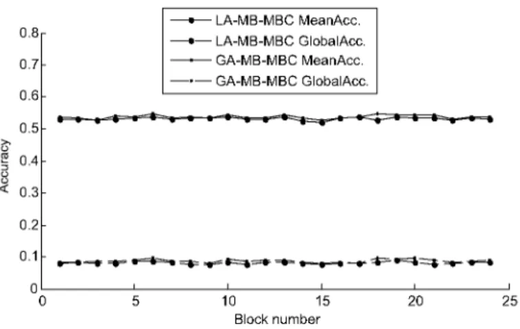
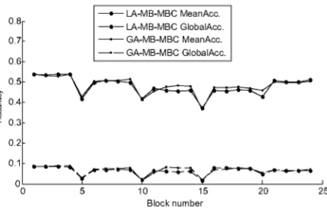
In addition, we plot in Figs 9-11 the mean and global accuracy curves for LA-MB-MBC and GA-MB-MBC algorithms, with A = 1 , block = 1000, and p equal to 0%, 20% and 50%, respectively. For each curve, the X-axis represents the block number, and the Y-axis represents the classification ac-curacy. Note that we limited this part to A = 1 , block = 1000, as similar conclusions are reached with the remaining configurations including different A and block size values.
In Fig. 9, we can observe that L A - M B - M B C and GA-MB-MBC curves are almost superposed showing the similar performance of both algorithms, as well as their resilience to false alarms.
In Figs 10 and 11, we can first notice that both algorithms perform well in detecting the change at blocks 5, 10, 15 and 20. With p = 20% (Fig. 10) the change is more gradual, whereas, in Fig. 11 with
p = 50%, the change is abrupt and more important fluctuations in predictive performance are present.
We can also see in Fig. 10 that LA-MB-MBC usually outperforms GA-MB-MBC in updating the MBC network and recuperating more quickly its performance. Nevertheless, with higher drift rate, i.e., p = 50%, GA-MB-MBC presents a slightly better performance than LA-MB-MBC.