Full text document (pdf)
Copyright & reuse
Content in the Kent Academic Repository is made available for research purposes. Unless otherwise stated all content is protected by copyright and in the absence of an open licence (eg Creative Commons), permissions for further reuse of content should be sought from the publisher, author or other copyright holder.
Versions of research
The version in the Kent Academic Repository may differ from the final published version.
Users are advised to check http://kar.kent.ac.uk for the status of the paper. Users should always cite the published version of record.
Enquiries
For any further enquiries regarding the licence status of this document, please contact:
[email protected]
If you believe this document infringes copyright then please contact the KAR admin team with the take-down information provided at http://kar.kent.ac.uk/contact.html
Citation for published version
Phan, Huy and Andreotti, Fernando and Cooray, Navin and Chén, Oliver Y. and De Vos, Maarten
(2018) Joint Classification and Prediction CNN Framework for Automatic Sleep Stage Classification.
IEEE Transactions on Biomedical Engineering . ISSN 0018-9294.
DOI
https://doi.org/10.1109/TBME.2018.2872652
Link to record in KAR
https://kar.kent.ac.uk/72662/
Document Version
Joint Classification and Prediction CNN Framework
for Automatic Sleep Stage Classification
Huy Phan
∗,
Member, IEEE,
Fernando Andreotti,
Member, IEEE,
Navin Cooray,
Student Member, IEEE,
Oliver Y. Ch´en,
Student Member, IEEE,
and Maarten De Vos
Abstract—Correctly identifying sleep stages is important in diagnosing and treating sleep disorders. This work proposes a joint classification-and-prediction framework based on convolu-tional neural networks (CNNs) for automatic sleep staging, and, subsequently, introduces a simple yet efficient CNN architecture to power the framework1. Given a single input epoch, the novel framework jointly determines its label (classification) and its neighboring epochs’ labels (prediction) in the contextual output. While the proposed framework is orthogonal to the widely adopted classification schemes, which take one or multiple epochs as contextual inputs and produce a single classification decision on the target epoch, we demonstrate its advantages in several ways. First, it leverages the dependency among consecutive sleep epochs while surpassing the problems experienced with the common classification schemes. Second, even with a single model, the framework has the capacity to produce multiple decisions, which are essential in obtaining a good performance as in ensemble-of-models methods, with very little induced computational overhead. Probabilistic aggregation techniques are then proposed to leverage the availability of multiple decisions. To illustrate the efficacy of the proposed framework, we conducted experiments on two public datasets: Sleep-EDF Expanded (Sleep-EDF), which consists of 20 subjects, and Montreal Archive of Sleep Studies (MASS) dataset, which consists of 200 subjects. The proposed framework yields an overall classification accuracy of 82.3% and 83.6%, respectively. We also show that the proposed framework not only is superior to the baselines based on the common classification schemes but also outperforms existing deep-learning approaches. To our knowledge, this is the first work going beyond the standard single-output classification to consider multitask neural networks for automatic sleep staging. This framework provides avenues for further studies of different neural-network architectures for automatic sleep staging.
Index Terms—sleep stage classification, joint classification and prediction, convolutional neural network, multi-task.
I. INTRODUCTION
Identifying the sleep stages from overnight Polysomnog-raphy (PSG) recordings plays an important role in diag-nosing and treating sleep disorders, which affects millions of people [1], [2]. Traditionally, this task has been done manually by experts via visual inspection which is tedious, time-consuming, and is prone to subjective error. Automatic sleep stage classification [3], that performs as well as manual H. Phan, F. Andreotti, N. Cooray, O. Y. Ch´en, and M. De Vos are with the Institute of Biomedical Engineering, University of Oxford, Oxford OX3 7DQ, United Kingdom.
∗Corresponding author:[email protected]
1The source code and the relevant experimental setup are available at http://github.com/pquochuy/MultitaskSleepNet for reproducibility.
Copyright (c) 2018 IEEE. Personal use of this material is permitted. However, permission to use this material for any other purposes must be obtained from the IEEE by sending an email to [email protected].
n+1 X X (b) (c) n+1 X X (a)
...
...
n-1 y yn+1...
...
...
...
n-1 y yn+1...
...
n+1 X X Xn+1 X...
...
...
...
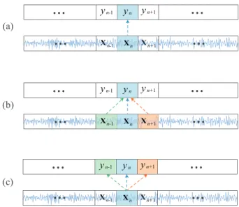
n X n y n y n X Xn+1 n-1 X n y n-1 y yn+1 n XFigure 1: Illustration of (a) the standard classification ap-proach, (b) the common classification approach with the contextual input of three epochs, and (c) the joint classification and prediction with the contextual output of three epochs proposed in this work.
scoring, can help to ease this task tremendously, therefore facilitating home monitoring of sleep disorders [4].
The guiding principle of automatic sleep staging is to split the signal into a sequence of epochs, each of which is usually 30 seconds long, and the classification is then performed epoch-by-epoch. In order to uncover a sleep stage at each epoch, proper features need to be derived from the signal, such as electroencephalography (EEG). Traditionally, many features have been designed based on prior knowledge of sleep. These hand-crafted features range from time-domain features [2], [5], [6] to frequency-domain features [6]–[9], via features derived from nonlinear processes [8], [10]–[12]. Using these features, the classification goal is often accomplished by conventional machine learning algorithms, such as Support Vector Machine
(SVM) [6], [13], k-nearest neighbors (k-NN) [7], Random
Forests [14]–[16].
The advent of deep learning and its astonishing progress in numerous domains have stimulated interest in applying them for automatic sleep staging. The power of deep networks lies in their great capability of automatic feature learning from data, thus avoiding the reliance on hand-crafted features. Significant progress on results obtained from different sleep staging benchmark using various deep learning techniques have been
reported [17]–[25], mirroring a relentless trend where learned features ultimately outperform and displace long-used hand-crafted features. CNN [26], [27], the cornerstone of deep learning techniques, has been frequently employed for the task [18]–[20]. The weight sharing mechanism at the convolutional layers forces the shift-invariance of the learned features and greatly reduces the model’s complexity, consequently leading to improvement of the model’s generalization [26]. Other network variants, such as Deep Belief Networks (DBNs) [28], Auto-encoder [21], Deep Neural Networks (DNNs) [23], have also been explored. Moreover, Recurrent Neural Networks (RNNs), e.g. Long Short-Term Memory (LTSM) [29], which are capable of sequential modelling, have been found efficient in capturing long-term sleep stage transition and are usually utilized to complement other network types, such as CNNs [17], [22] and DNNs [23]. Standalone RNNs have also been exploited for learning sequential features of sleep [25], [30], [31]. The classification is usually performed therein by the net-works in an end-to-end fashion [18]–[20]; a separate classifier, such as SVM, can be used alternatively [25], [32].
II. MOTIVATION ANDCONTRIBUTIONS
A. Motivation
Sleep is a temporal process with slow stage transitions, implying continuity of sleep stages and strong dependency between consecutive epochs [33]–[35]. For instance, out of 228,870 epochs in the entire MASS dataset [36] used in this
work, 83.3% pairs of adjacent epochs have the same label.
The ratio is still as high as 79.3%, when two epochs are
separated by one epoch. This nature of sleep has inspired a widely adopted practice in neural-network-based sleep staging
systems, namely the use of contextual input that augments a
target epoch by its surrounding epochs (many-to-one) in the
classification task [17], [18], [20], [22]. Common input context size is of three and five epochs [18], [20], [21], [37]. This classification scheme can also be interpreted as an extension of the standard classification setup, i.e. determining the sleep
stage corresponding to a single epoch of input signals (
one-to-one) [24], [25], [38]. Figure 1 (b) provides a schematic presentation of contextual input of three epochs in comparison with the standard one-to-one classification approach in Fig-ure 1 (a). While multiple-epoch input does not always provide performance gains, as shown in our experiments, it poses
a problem of inherent modelling ambiguity. That is, when
training a network with contextual input, such as three epochs illustrated in Figure 1 (b), it remains unclear whether the network is truly modelling the class distribution of the target epoch at the center or that of the left and right neighbor. In our experiment, such a network (i.e. the many-to-one baseline
in Section V-C) achieves an accuracy of82.1%in determining
the labels of the center epochs. However, when aligning the network output with those labels of the left and right neighbor,
the accuracy is just marginally lower, reaching 81.1% and
80.8%, respectively. Last but not least, the contextual input causes the network’s computational complexity increase at a linear scale due to the enlarged input size.
In this work, we formulate sleep staging as a joint clas-sification and prediction problem. In other words, this is
equivalent to a one-to-manyproblem, which is an extension
of the standard one-to-one classification scheme while being orthogonal to the common many-to-one classification scheme. With this new formulation, given a single target epoch as input, our objective is to simultaneously determine its label (classification) and its neighboring epochs’ labels (prediction)
in the contextual output, as demonstrated in Figure 1 (c). By
classification, we mean determining the label of an epoch given its information. In contrast, prediction implies determin-ing the label of an epoch without knowdetermin-ing its information. The rationale behind this idea is that, given the strong dependency of consecutive epochs, using information of an epoch, we should be able to infer the label of its neighbors. The major benefit of the joint classification and prediction formulation are two-fold. First, with the single-epoch input, the employed model does not experience the modelling ambiguity and the computational overhead induced by the large contextual input as previously discussed. Second, the employed model can produce an ensemble of decisions, which is the key in our obtained state-of-the-art performance, with a negligible induced computational cost. Ensemble of models [39], [40], a well-established method to improve the performance of a machine learning algorithm, has been found generalizable to automatic sleep staging, evidenced by conventional methods [6], [13], [41] and recently developed deep neural networks [17]. However, building many different models on the same data for model fusion is cumbersome and costly. Opposing to ensemble of models [6], [13], [17], [41], in our joint classifi-cation and prediction formulation, the ensemble of decisions
is produced with a single multi-task model. Afterwards, an
aggregation method can be used to fuse the ensemble of decisions to produce a reliable final decision.
We further proposed a CNN framework to deal with the joint problem. Although the proposed framework is generic in the sense that any CNN can fit in, we employ a simple CNN archi-tecture with time-frequency image input. The efficiency of this architecture for automatic sleep staging was demonstrated in our previous work [24]. To suit the task of joint classification and prediction, we replace the CNN’s canonical softmax layer
with a multi-task softmax layer and introduce the multi-task
lossfunction for network training. Without confusion, we will
refer to the proposed framework as multi-task framework, joint classification and prediction framework, and one-to-many framework interchangeably throughout this article.
B. Contributions
The main contributions of this work are as follows. (i) We formulate automatic sleep staging as a joint classi-fication and prediction problem. The new formulation avoids the shortcomings of the common classification scheme while improving modelling performance.
(ii) A CNN framework is then proposed for the joint problem. To that end, we present and employ a simple and efficient CNN coupled with a multi-task softmax layer and the multi-task loss function to conduct joint classification and prediction.
(iii) We further propose two probabilistic aggregation meth-ods, namely additive and multiplicative voting, to leverage
raw signals time-frequency image
Multi-task CNN feature
extraction and predictionclassification
EEG EOG EMG epoch n n
y
τ − ny
...
...
y
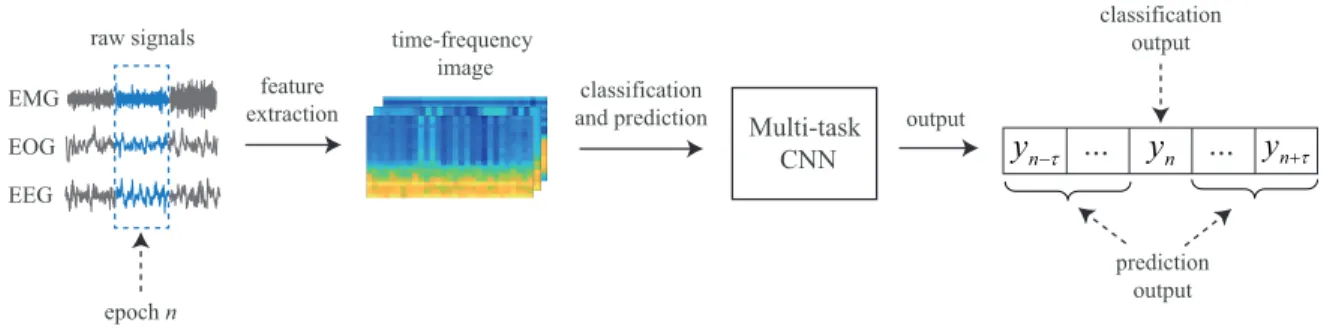
n+τ output classification output prediction output Figure 2: Overview of the proposed joint classification and prediction framework. ensemble of decisions available in the proposed framework.(iv) Performance-wise, we demonstrate experimentally good performance on two publicly available datasets: Sleep-EDF [42], [43] with 20 subjects and MASS [36], a large sleep dataset with 200 subjects.
III. EVALUATIONDATASETS
We used two public datasets: Sleep-EDF Expanded (Sleep-EDF) and Montreal Archive of Sleep Studies (MASS) in this work and conducted analyses under both unimodal (i.e. single-channel EEG) and multimodal conditions (i.e combinations of EEG, EOG, and EMG channels). It should be noted that even though we selected the typical EEG, EOG, and EMG channels in our analyses, the proposed framework, however, can be used straightforwardly to study other signal modalities.
A. Sleep-EDF Expanded (Sleep-EDF)
Sleep-EDF dataset [42], [43] consists of two subsets: (1) Sleep Cassette (SC) subset consisting of 20 subjects aged 25-34 aiming at studying the age effects on sleep in healthy
subjects and (2) Sleep Telemetry (ST) subject consisting of
22 Caucasian subjects for study temazepam effects on sleep.
We adopted the SC subset in this study. PSG recordings,
sampled at 100 Hz, of two subsequent day-night periods are available for each subject, except for one subject (subject 13) who has only one-night data. Each 30-second epoch of the recordings was manually labelled by sleep experts according
to the R&K standard [44] into one of eight categories {W,
N1, N2, N3, N4, REM, MOVEMENT, UNKNOWN}. Similar
to previous works [20]–[22], N3 and N4 stages were merged into a single stage N3. MOVEMENT and UNKNOWN were excluded. Since full EMG recordings are not available, we only used the Fpz-Cz EEG and the EOG (horizontal) channels
in our experiments. Only the in-bed parts (from lights off
time to lights on time) of the recordings were included as
recommended in [20], [21], [45], [46]. B. Montreal Archive of Sleep Studies (MASS)
MASS comprises whole-night recordings from 200 subjects (97 males and 103 females with an age range of 18-76 years). These recordings were pooled from different hospital-based sleep laboratories. The available cohort 1 was divided into five subsets of recordings, SS1 - SS5. As stated in the seminal work [36], heterogeneity between subsets is expected. Opposing to the majority of previous works which targeted only one
homogeneous subset of the cohort [22], [23], we experimented with all five subsets. Each epoch of the recordings was manually labelled by experts according to the AASM standard [33] (SS1 and SS3) and the R&K standard [44] (SS2, SS4, and
SS5). We converted them into five sleep stage {W, N1, N2,
N3, and REM} as suggested in [45], [46]. Those recordings
with 20-second epochs were converted into 30-second ones by including 5-second segments before and after each epoch. We adopted and studied combinations of the C4-A1 EEG, an average EOG (ROC-LOC), and an average EMG (CHIN1-CHIN2) channels in our experiments. The signals, originally sampled at 256 Hz, were downsampled to 100 Hz.
IV. JOINTCLASSIFICATION ANDPREDICTIONCNN
FRAMEWORK A. Overview
The proposed framework, with a schematic illustration shown in Figure 2, can be described in a stage-wise
fash-ion. The raw signals of a certain epoch index n are first
transformed into log-power spectra. The spectra are then pre-processed for frequency smoothing and dimension reduction using frequency-domain filter banks. The resulting channel-specific images are then stacked to form a multi-channel
time-frequency image, denoted as Xn. Subsequently, a multi-task
CNN is exercised on the multi-channel time-frequency image for joint classification and context prediction. The former
task is to maximize the conditional probability P(yn|Xn)
which characterizes the likelihood of a sleep stage yn ∈
L={1,2, . . . , Y}, whereLdenotes the label set ofY sleep stages. The latter one is to maximize the conditional proba-bilities (P(yn−τ|Xn), . . . , P(yn−1|Xn), P(yn+1|Xn), . . . , P(yn+τ|Xn))of the neighboring epochs in the output context
size of 2τ + 1. The labels of the epochs in the output
context, where(yn−τ, . . . , yn, . . . , yn+τ), can be obtained by probability maximization.
Formally, under this joint classification and prediction for-mulation, the CNN performs the one-to-many mapping
ˆ
F:Xn7→(yn−τ, . . . , yn, . . . , yn+τ)∈ L
2τ+1 . (1) Note that the order of the epochs in the neighborhood is encoded by the order of the output labels. This formulation is orthogonal to the common classification one with contextual
input of size2τ+ 1, in which a network performs the
many-to-one mapping
Both formulations (1) and (2) can be interpreted as different extensions of the standard one-to-one classification scheme [24], [25], [38]. They will reduce to the standard one when
τ = 0. However, with our joint classification and prediction
formulation, at a certain epoch index n there exists an
en-semble of exact 2τ+ 1decisions, wherein one classification
decision made by itself (i.e. Xn) and2τ prediction decisions made by its neighbors (Xn−τ, . . . ,Xn−1,Xn+1, . . . ,Xn+τ). These decisions can be aggregated to form the final decision that is generally better that any individual ones.
B. Time-Frequency Image Representation
Given a 30-second signal epoch (i.e. EEG, EOG, or EMG), we firstly transform it into a power spectrum using short-time Fourier transform (STFT) with a window size of two seconds and 50% overlap. Hamming window and 256-point Fast Fourier Transform (FFT) are used. The spectrum is then converted to logarithm scale to produce a log-power spectrum
image of sizeF×T, where F = 129andT = 29.
For frequency smoothing and dimension reduction, the spectrum is filtered by a frequency-domain filter bank. Any frequency-domain filter bank, such as the regular triangular one [24], could serve this purpose. However, it is more favorable to learn the filter bank specifically for the task at hand. Our recent works in [24], [25] demonstrated that a filter bank learned by a DNN in a discriminative fashion is more competent than the regular one in automatic sleep staging. The learned filter bank is expected to emphasize the subbands that are more important for the task and attenuate those less impor-tant. Hence, we use the filter bank pretrained with a DNN for preprocessing here. One such filter bank withM = 20filters is learned for each EEG, EOG, and EMG channel. Filtering the
log-power spectrum image reduces its size to M ×T. When
multiple channels are used, we obtain one such time-frequency image for each channel. For generalization, we denote the
time-frequency image as X ∈ RP×M×T where P denotes
the number of channels.P = 1,2,3 is equivalent to the cases
when {EEG}, {EEG, EOG}, and {EEG, EOG, EMG} are
employed, respectively.
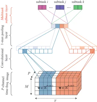
C. Multi-Task CNN for Joint Classification and Prediction Our recent work [24] presented a simple CNN architecture that was shown efficient for sleep staging. We adapt this architecture here by tailoring the last layer, i.e. the multi-task softmax layer, to perform joint classification and prediction. The proposed CNN architecture is illustrated in Figure 3. Opposing to typical deep CNNs [17], [18], [20], [22], the proposed CNN consists of only three layers: one over-time
convolutional layer, one pooling layer, and one multi-task
softmax layer. This simple architecture has three main char-acteristics. First, similar to those in [22], [47], [48], its con-volutional layer simultaneously accommodates concon-volutional kernels with varying sizes, and is therefore able to learn
features at different resolutions. Second, the exploited 1-max
pooling strategy at the pooling layer is more suitable for capturing theshift-invarianceproperty of temporal signals than the common subsampling pooling since a particular feature
P-channel time-freq. image Convolutional layer 1-max pooling layer Multitask softmax layer T M P P×M×3 ∈R w w∈RP×M×5
...
...
subtask i subtask j subtask k
Figure 3: Illustration of the proposed multi-task CNN archi-tecture. The convolution layer of the CNN consists of two
filter sets with temporal widthsw= 3andw= 5. Each filter
set has two individual filters. The colors of the output layer indicate different subtasks jointly modelled by the network.
could occur at any temporal position rather than in a local region of the input signal [47]–[49]. Third, opposing to the canonical softmax, the multi-task softmax layer is adapted to suit the joint classification and prediction. Furthermore, the multi-task loss is introduced for network training.
Assume that we obtain a training set
S = nX(i)ni,(y (i) ni−τ, . . . ,y (i) ni, . . . ,y (i) ni+τ) oN i=1 of
size N from the training data. An epochi is represented by
the multi-channel time-frequency image X(i)ni ∈ R
P×M×T
as described in IV-B and ni denotes the corresponding
index of the epoch in the original signal. Each epoch i is
associated with the sequence of one-hot encoding vectors
(y(i)ni−τ, . . . ,y (i) ni, . . . ,y
(i)
ni+τ)which represent the sleep stages
of the epochs in the context [ni−τ, ni+τ] of size 2τ+ 1. We use this training set to train the multi-task CNN for joint classification and context prediction.
1) Over-Time Convolutional Layer: Each 3-dimensional
filter w ∈ RP×M×w of the convolutional layer has the
temporal size ofw < T while the frequency and channel size
entirely cover the frequency and channel dimension of a multi-channel time-frequency image input. The filter is convolved
with the input image over time with a stride of 1. ReLU
activation [50] is then applied to the feature map.
The CNN is designed to have R filter sets with different
temporal widths w to capture features at multiple temporal
resolutions. Each filter consists of Q different filters of the same temporal width to allow the CNN to learn multiple complementary features. As a result, the total number of filters isQ×R.
2) 1-Max Pooling Layer: We employ 1-max pooling func-tion [48], [49] on a feature map produced by convolving a
) | ( n n+τ P y X
...
P(yn+τ|Xn+τ)...
P(yn+2τ|Xn+τ)...
...
...
...
...
...
) | ( n P yn+τ X ) | ( n n P y X ) | ( n P yn−τX ) | ( n n−τ P y X ) | ( n−τ P yn−τX ) | ( n−τ P yn−2τXFigure 4: Ensemble of decisions available at the epoch index nmade by the epochs Xi in the neighborhood [n−τ, n+τ],
i.e. n−τ ≤i≤n+τ.
filter over an input image to retain the most prominent feature.
Pooling all feature maps of Q×R filters results in a feature
vector of size Q×R.
With the over-time convolution layer coupled with the 1-max pooling layer, the CNN functions as a template learning and matching algorithm. The convolutional filters play the role of time-frequency templates that are tuned for the task at hand. Convolving a filter through time can be interpreted as template matching operation, resulting in a feature map that indicates how well the template is matched to different parts of the input image. In turn, 1-max pooling retains a single maximum value, i.e. the maximum matching score, of the feature map as the final feature.
3) Multi-Task Softmax Layer: Opposing to a classification network that typically uses the canonical softmax layer for classification, we propose a multi-task softmax layer to suit joint classification and prediction. The idea is that the network should be penalized for both misclassification and mispredic-tion on a training example. The classificamispredic-tion and predicmispredic-tion
errors on a training example iis computed as the sum of the
cross-entropy errors on the individual subtasks: E(i)(θ) =
ni+τ
X
n=ni−τ
yn(i)logyˆn(i)(θ), (3)
where θ andyˆ denote the network parameters and the
prob-ability distribution outputted by the CNN, respectively. The network is trained to minimize the multi-task
cross-entropy error over N training samples:
E(θ) =−1 N N X i=1 E(i)(θ) +λ 2kθk 2 2. (4)
Here, λdenotes the hyper-parameter that trades off the error
terms and theℓ2-norm regularization term. For further
regular-ization, dropout[51] is also employed. The network training
is performed using theAdamoptimizer [52].
D. Ensemble of Decisions and Aggregation
As previously mentioned, one major advantage of the pro-posed framework is the capacity to produce multiple decisions on a certain epoch even with a single model (the multi-task CNN in this case). Practically, the classification and prediction outputs on a certain epoch may be inconsistent as in ensemble-of-models methods [39], [40]; aggregation of these multi-view decisions is necessary to derive a more reliable one. To that
end, we study two probabilistic aggregation schemes: additive and multiplicative voting.
Let P(yn|Xi) denote the estimated probability output on
the sleep stage yn ∈ Lat the epoch indexngiven the epoch
Xi in the neighborhood[n−τ, n+τ], i.e.n−τ ≤i≤n+τ, as illustrated in Figure 4. The likelihoodP(yn) obtained by additive and multiplicative voting is given by
P(yn) = 1 2τ+ 1 n+τ X i=n−τ P(yn|Xi), (5) P(yn) = 1 2τ+ 1 n+τ Y i=n−τ P(yn|Xi), (6) respectively. Eventually, the predicted label ynˆ is determined by likelihood maximization:
ˆ
yn = arg max
yn
P(yn), foryn∈ L. (7) Between the two aggregation schemes, the multiplicative one favors likelihoods of categories with consistent decisions and suppresses likelihoods of those categories with diverged decisions stronger than the additive counterpart [53].
V. EXPERIMENTS
We aim at achieving several goals in the conducted exper-iments. Firstly, we prove empirically the feasibility of pre-dicting labels of the neighboring epochs in the output context concurrently with classifying the current one. Secondly, we demonstrate the advantages of the joint classification and prediction (i.e. many-to-one) formulation over the commonly adopted many-to-one scheme as well as the standard one-to-one classification scheme. Thirdly, we provide performance comparison with various developed baseline systems as well as other deep-learning approaches recently proposed for sleep staging to illustrate the proposed framework’s efficiency. A. Experimental Setup
For Sleep-EDF, we conducted leave-one-subject-out cross validation. At each iteration, 19 training subjects were further divided into 15 subjects for training and 4 subject for valida-tion. For MASS, we performed 20-fold cross validation on the MASS dataset. At each iteration, 200 subjects were split into training, validation, and test set with 180, 10, and 10 subjects, respectively. The sleep staging performance over 20 folds will be reported for both datasets.
Table I: Parameters of the proposed CNN.
Parameter Value
Filter widthw {3,5,7}
Number of filtersQ varied Output context size 3
Dropout 0.2
λfor regularization 10−3
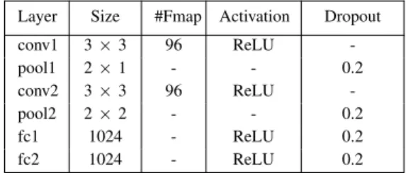
Table II: The parameters of the deep CNN baseline. Layer Size #Fmap Activation Dropout
conv1 3×3 96 ReLU -pool1 2×1 - - 0.2 conv2 3×3 96 ReLU -pool2 2×2 - - 0.2 fc1 1024 - ReLU 0.2 fc2 1024 - ReLU 0.2 B. Parameters
The parameters associated with the proposed CNN are given
in Table I. We varied the number of convolutional filters Q
of the CNN in the set {100, 200, 300, 400, 500, 1000} to
investigate its influence. Furthermore, we experimented with
the output context size of 3 (equivalent to τ = 1). Influence
of this parameter will be further discussed in Section VI.
The network implementation was based on Tensorflow
framework [54]. Graphic card NVIDIA GTX 1080 Ti was used for network training. The network was trained for 200 epochs with a batch size of 200. The learning rate was set to10−4for
theAdamoptimizer. During training, the network that yielded
the best overall accuracy on the validation set was retained for evaluation. Furthermore, we always randomly generated a data batch to have an equal number of samples for all sleep stages to mitigate the class imbalance issue commonly seen in sleep data.
C. Baseline Systems
To manifest the advantages offered by the proposed frame-works, we constructed two baseline frameworks for compari-son:
• One-to-one: this baseline complies with the standard
classification setup, taking a single epoch as input and producing a single decision on its label.
• Many-to-one: this baseline conforms to the commonly
adopted scheme with contextual input and outputs a single decision on a target epoch. We fixed the contextual input size to 3, i.e. we augmented a target epoch with two nearest neighbors on its left- and right-hand side. Both baseline frameworks were designed to maintain com-mon experimental settings as those of the proposed one-to-many framework, i.e. the CNN architecture, the learned filter bank, etc. However, it is necessary to use the canonical softmax layer and the standard cross-entropy loss for their classification-only purpose.
We also developed and repeated the experiments with a typical deep CNN architecture as an alternative to the proposed
CNN described in Section IV-C. This deep CNN baseline consists of 6 layers (2 convolutional layers, 2 subsampling layers, and 2 fully connected layers) with their parameters characterized in Table II. For simplicity, we refer to our proposed CNN as 1-max CNN to distinguish from the deep CNN baseline. With these experiments, our goal is to show the generalizability of the proposed framework regardless the network base as well as the efficacy of the 1-max CNN in comparison to a typical deep CNN architecture.
D. Experimental Results
1) Classification vs prediction accuracy: In this experi-ment, we seek to empirically validate the proposed framework by demonstrating the feasibility of context prediction. Since
we employed the output context size of3, without confusion,
let us refer to the network’s subtasks as classification, left prediction, andright prediction, which correspond to decisions on the input epoch, its left neighbor, and its right neighbor.
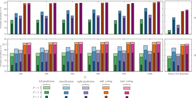
We show in Figure 5 the accuracy rates of classification, left prediction, and right prediction subtasks obtained by the
1-max CNN (with varying number of convolutional filtersQ)
and the deep CNN baseline with the different number of input
modalities P. Unlike the classification subtask, the CNNs do
not have access to the signal information of the left and right neighboring epochs. As a result, inference for their labels relies solely on their dependency with the input epoch. It can be expected that the accuracy rates of the left and right prediction subtasks are lower than that of the classification subtask in most of the cases. Nevertheless, overall both CNNs maintain a good accuracy level in prediction relative to the classification accuracy, especially in multimodal cases (e.g.P = 2for
Sleep-EDF and P = 3 for MASS). More specifically, averaging
over all Q and P, the left and right prediction accuracies
of the 1-max CNN are only 2.9% and 1.4% lower than the
classification accuracy on Sleep-EDF whereas the respective
gaps of 2.2% and 1.3% are seen in MASS. Similar patterns
can also be seen with the deep CNN baseline with the graceful
degradation of 4.0% and 2.5% in Sleep-EDF and 3.3% and
2.2%in MASS correspondingly. These results strengthen the
assumption about the dependency between neighboring PSG epochs and consolidate the feasibility of joint classification and prediction modelling.
2) Advantages of the joint classification and prediction: Figure 5 also highlights the performance improvements ob-tained by the joint classification and prediction framework after the aggregation step in comparison to individual subtasks.
Averaging over all P andQ, the 1-max CNN with additive
voting leads to2.8% and4.5%absolute accuracy gains over
the classification subtask’s accuracy on Sleep-EDF and MASS, respectively. The gains yielded by the multiplicative voting are even better, reaching 3.0% and 4.7%, respectively.
Ac-cordingly, the deep CNN baseline produces 2.2% and 2.5%
absolute gains with additive voting and2.6% and2.8% with
multiplicative voting on the two datasets. Between two voting schemes, the performance gain of the multiplicative one is slightly better than that of the additive counterpart with a
72 74 76 78 80 82 Overall accuracy (%) 100 200 300 400 500 1000 Q 70 72.5 75 77.5 80 82.5 85 Overall accuracy (%) Deep CNN Baseline (a) (b) mul. voting add. voting right prediction classification left prediction P = 3 P = 2 P = 1
Figure 5: Accuracies of the left prediction subtask, classification subtask, right prediction subtask, multi-task with additive (add.) voting, and multi-task with multiplicative (mul.) voting obtained with an output context size of 3 (τ= 1) and different
number of modalities P. (a) Sleep-EDF and (b) MASS.
76 78 80 82
Overall accuracy (%)
one-to-one many-to-one one-to-many
Deep CNN baseline 1-max CNN 0.3
0.2 0.1 0
Training time (hours)
80 81 82 83 84 Overall accuracy (%)
Deep CNN baseline 1-max CNN 4
3 2 1 0
Training time (hours)
(a)
(b)
(c)
(d)
Sleep-EDF MASS
Figure 6: The overall classification accuracy (a)-(c) and the amount of training time (b)-(d) of the proposed framework in comparison with those of the one-to-one, and many-to-one schemes on the first cross-validation fold. We commonly set Q= 1000whileP = 2for Sleep-EDF andP = 3for MASS.
To demonstrate the advantages of the proposed framework over the common classification schemes, we further compare its performance and computational complexity with the one-to-one and many-one-to-one baseline schemes described in Section V-C. For simplicity, we utilized all available modalities (i.e.
P = 3) in this experiment and made use of
multiplicative-voting aggregation in the proposed framework. Additionally,
we set the number of convolutional filtersQ= 1000when the
1-max CNN was employed.
Figure 6 depicts the overall accuracy obtained by the three frameworks and their computational complexity in terms of the training time. Note that we only included the training time of the first cross-validation fold as a representative here and the training time was expected to scale linearly with
the amount of training data. Four important points should be noticed from the figure. Firstly, contextual input does not always help as the many-to-one baseline with the 1-max CNN
experiences a performance drop of 0.6% absolute compared
to the one-to-one on MASS compared to the one-to-one on MASS although it improves accuracy rates in other cases. Secondly, the proposed one-to-many framework consistently outperforms its counterparts. Adopting the 1-max CNN as the base, our framework outperforms the one-to-one and
many-to-one opponents with 2.5% and 0.2% absolute in
Sleep-EDF and 1.0% and 1.6% absolute in MASS, respectively.
Similar gains of 2.5% and 1.0% in Sleep-EDF; 1.7% and
0.3% in MASS are achieved when the deep CNN baseline
is used. Thirdly, between the network bases, the 1-max CNN surpasses the deep CNN baseline with an improvement of
2.6% absolute in Sleep-EDF and 0.9% absolute in MASS
although its architecture is much simpler. Fourthly, concerning the computational complexity, three times larger input of the many-to-one baseline roughly triples the training time compared to that of the one-to-one. For instance, 4.0 hours versus 1.36 hours in MASS can be seen with the 1-max CNN. Differently, with the training time of1.6hours. Using the same network, the proposed framework only increases computing
time by as small as0.2 hours. The training time of the deep
CNN baseline also exposes similar patterns.
3) Performance comparison: Table III provides a compre-hensive performance comparison on the experimental dataset using different metrics, including overall accuracy, kappa index κ, average specificity, average sensitivity, and average macro F1-score (MF1). The comparison covers all combi-nations of different frameworks (i.e. the proposed and the baselines) and network bases (i.e. the proposed 1-max CNN
Table III: Performance comparison of different systems developed in this work. We marked in bold the figures where the combination of the one-to-many framework and 1-max CNN outperforms all other opponents.
P= 1(EEG only) P = 2(EEG + EOG) P = 3(EEG + EOG + EMG) Acc. κ MF1 Sens. Spec. Acc. κ MF1 Sens. Spec. Acc. κ MF1 Sens. Spec.
Sleep-EDF
One-to-many + 1-max CNN 81
.9 0.74 73.8 73.9 95.0 82.3 0.75 74.7 74.3 95.1 One-to-one + 1-max CNN 79.8 0.72 72.0 72.4 94.6 79.7 0.72 72.2 72.8 94.6 Many-to-one + 1-max CNN 80.9 0.73 73.6 74.2 94.9 82.1 0.75 75.4 75.4 95.1 One-to-many + deep CNN baseline 79.3 0.71 69.7 70.2 94.2 79.7 0.71 71.2 70.9 94.3 One-to-one + deep CNN baseline 76.7 0.67 67.6 68.6 93.7 77.1 0.68 69.3 69.8 93.8 Many-to-one + deep CNN baseline 78.3 0.69 70.7 71.1 94.1 78.7 0.70 71.8 72.4 94.2
MASS
One-to-many + 1-max CNN 78
.6 0.70 70.6 71.2 94.1 82.5 0.75 76.1 75.8 95.0 83.6 0.77 77.9 77.4 95.3 One-to-one + 1-max CNN 75.9 0.67 69.6 71.1 93.7 80.7 0.73 74.9 75.5 94.8 82.7 0.75 77.6 77.8 95.1 Many-to-one + 1-max CNN 76.3 0.67 69.8 71.3 93.8 80.9 0.73 75.1 75.5 94.8 82.1 0.75 76.6 76.9 95.0 One-to-many + deep CNN baseline 78.0 0.69 69.8 70.1 93.8 81.9 0.74 75.2 74.7 94.8 82.7 0.75 76.9 76.3 95.0 One-to-one + deep CNN baseline 74.5 0.65 68.4 70.0 93.4 79.2 0.71 73.5 74.3 94.4 81.0 0.73 76.4 77.4 94.9 Many-to-one + deep CNN baseline 77.4 0.68 71.6 72.8 94.0 81.2 0.73 76.0 76.4 94.8 82.4 0.75 78.2 78.9 95.2
Table IV: Performances of the proposed method compared to previous methods on the Sleep-EDF dataset. Notice the large variation in the accuracy rate due to the differences in experimental setup. Top accuracy rates, such as in Aboalayonet al.[3], Alickovic & Subasi [13], and Dimitriadiset al.[55], are likely biased by nonindependent testing and usage of entire recordings rather than only in-bed data (cf. V-D3 for further detail).
Method Input channel Feature type Subjects Independent testing
In-bed data only
Overall accuracy
This work Multitask 1-max CNN Fpz-Cz + hor. EOG learned 20 SC yes yes 82.3
This work Multitask 1-max CNN Fpz-Cz learned 20 SC yes yes 81.9
Phanet al.[24] 1-max CNN Fpz-Cz learned 20 SC yes yes 79.8
Phanet al.[25] Attentional RNN Fpz-Cz learned 20 SC yes yes 79.1
Andreottiet al.[38] ResNet Fpz-Cz + hor. EOG learned 20 SC yes yes 76.8
Tsinaliset al.[21] Deep auto-encoder Fpz-Cz hand-crafted 20 SC yes yes 78.9
Tsinaliset al.[20] Deep CNN Fpz-Cz learned 20 SC yes yes 74.8
Suprataket al.[22] Deep CNN + RNN Fpz-Cz learned 20 SC yes no 82.0
Alickovic & Subasi [13] Ensemble SVM Pz-Oz hand-crafted 10 SC + 10 ST yes no 91.1
Sanderset al.[56] Decision trees Fpz-Cz hand-crafted 10 ST yes no 75.0
Dimitriadiset al.[55] k-NN Fpz-Cz hand-crafted 20 SC yes no 94.4
Mikkelsen & De Vos [18] Deep CNN Fpz-Cz + hor. EOG learned 20 SC no yes 84.0
Imtiazet al.[16] Ensemble SVM Fpz-Cz + Pz-Oz hand-crafted 20 SC + 22 ST no yes 78.9
Munket al.[57] GMM Pz-Oz hand-crafted 19 SC no no 73.2
Rodr´ıguez-Soteloet al.[58] k-NN Fpz-Cz + Pz-Oz hand-crafted 20 SC no no 80.0
Aboalayonet al.[3] Decision trees Fpz-Cz + Pz-Oz hand-crafted 20 SC no no 93.1
Table V: Performances of the proposed method compared to previous methods on the MASS dataset.
Method Input channel Feature type Subjects Independent testing
Overall accuracy
This work Multitask 1-max CNN C4-A1 + ROC-LOC + CHIN1-CHIN2 learned 200 yes 83.6
This work Multitask 1-max CNN C4-A1 + ROC-LOC learned 200 yes 82.5
This work Multitask 1-max CNN C4-A1 learned 200 yes 78.6
Chambon et al.2[37] Deep CNN C4-A1 + ROC-LOC + CHIN1-CHIN2 learned 200 yes 79.9 DeepSleepNet12[22] Deep CNN C4-A1 + ROC-LOC + CHIN1-CHIN2 learned 200 yes 80.7 Tsinalis et al.2[20] Deep CNN C4-A1 + ROC-LOC + CHIN1-CHIN2 learned 200 yes 77.9
Andreottiet al.[38] ResNet C4-A1 + ROC-LOC + CHIN1-CHIN2 learned 200 yes 79.4
Chambonet al.[37] Deep CNN 6 EEG + 2 EOG + 3 EMG learned 61 (SS3 only) yes 83.0
Suprataket al.[22] Deep CNN F4-EOG (left) learned 62 (SS3 only) yes 81.5
Donget al.[23] DNN F4-EOG (left) learned 62 (SS3 only) yes 81.4
Donget al.[23] Random Forests F4-EOG (left) hand-crafted 62 (SS3 only) yes 81.7
Donget al.[23] SVM F4-EOG (left) hand-crafted 62 (SS3 only) yes 79.7
and the deep CNN baseline). As can be seen, the proposed one-to-many framework powered by the 1-max CNN (one-to-many + 1-max CNN) outperforms other combinatorial sys-2Our implementation. Source code is also available at http://github.com/ pquochuy/MultitaskSleepNet
tems presented in this work on both datasets and over different combinations of modalities. There are occasional exceptions where using the 1-max CNN in the baseline frameworks yields
marginally better average MF1 and Sensitivity than
one-to-many + 1-max CNN, such as on MASS withP = 3; however,
To see an overall picture, in Tables IV and V we relate the proposed method’s accuracy to those reported by previous works on the two datasets. With this comprehensive compar-ison, we also aim at providing a benchmark for future work.
As can be seen from Table IV, the results on Sleep-EDF vary noticeably due to the lack of standardization in experimental setup. We observe two factors that greatly affects performance on this dataset: (1) independent/dependent testing
and (2) whether or not using only in-bedparts of the
record-ings as recommended in [16], [20], [21], [46]. Dependent testing happens when data of a test subject is also involved
in training, such as in Aboalayon et al. [3], and biases the
evaluation results. In addition to in-bed parts (i.e. from lights
off time to lights on time [46]), many previous studies also
included other parts, such as in Supratak et al.[22], or even
entire recordings, such as in Dimitriadis et al. [55] and in
Alickovic & Subasi [13], into their experiments. These
add-on data, which are mainly Wakeepochs, often boost the
per-formance as Wake, in general, is easier to be recognized than
other sleep stages. Therefore, the performance comparison is improper unless two methods use a similar experimental setup. With respect to this, the proposed method outperforms other competitors that commonly used independent testing and in-bed data only. It should be noted that these results do not cover a large body of studies on the early version of Sleep-EDF dataset [42], [43] which consists of only 8 PSG recordings.
A few recent attempts has evaluated automatic sleep staging on a subset [22], [23], [37] rather than the entire 200 subjects of the MASS dataset. The discrepancy in data makes a direct comparison between their results and ours inappropriate. To avoid possible mismatch in experimental setup, we re-implemented DeepSleepNet [22] and the deep CNN
archi-tecture proposed by Chambon et al. [37], both of which
recently reported the state-of-the-art results on the MASS subset SS3, for a compatible comparison. Note that we ex-perimented with DeepSleepNet1 (CNN) in [22] here, and will leave DeepSleepNet2 (CNN combined with RNN for long-term context modelling) for future work. In addition, we also
implemented the deep CNN proposed by Tsinalis et al. [20]
which demonstrated good performance on Sleep-EDF. While our developed baselines (cf. Table III) are more efficient than these networks under the common experimental setup used in this work, the improvements by the proposed multitask 1-max CNN are most prominent, as can be seen from Table V. More specifically, compared to the best opponent, DeepSleepNet
[22], a margin of2.9%on overall accuracy is obtained when
all three adopted channels (P = 3) were used.
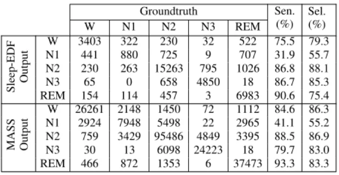
For completeness, we show in Table VI the confusion matrices and class-wise performance in terms of sensitivity and selectivity [45] obtained by the proposed one-to-many framework with the 1-max CNN base. Particularly, one may notice modest performance on N1 stage, which has been proven challenging to be correctly recognized [20], [22], [24], [25] due to its similarities with other stages and its infrequency. Possibilities for improvement would be to over-sample the under-present class during training and to explore weighting schemes for a network’s loss [31], [59] so that the network is penalized stronger if making errors on this infrequent class
Table VI: Confusion matrices and class-wise performance (sensitivity and selectivity) obtained by the proposed one-to-many framework with the 1-max CNN base.
Groundtruth Sen. (%) Sel. (%) W N1 N2 N3 REM Sleep-EDF Output W 3403 322 230 32 522 75.5 79.3 N1 441 880 725 9 707 31.9 55.7 N2 230 263 15263 795 1026 86.8 88.1 N3 65 0 658 4850 18 86.7 85.3 REM 154 114 457 3 6983 90.6 75.4 MASS Output W 26261 2148 1450 72 1112 84.6 86.3 N1 2924 7948 5498 22 2965 41.1 55.2 N2 759 3429 95486 4849 3395 88.5 86.9 N3 30 13 6098 24223 18 79.7 83.0 REM 466 872 1353 6 37473 93.3 83.3
than other ones. We further provide alignment of ground-truth and system-output hypnograms for one subject of the MASS dataset in Figure 7.
VI. DISCUSSION
In this section, we investigate the causes of the proposed framework’s performance improvement over the baseline ones. Furthermore, the proposed framework encompasses several in-fluential factors, such as the number of convolutional filtersQ
of the 1-max CNN, the number of input modalitiesP, and the
output context size. We will discuss and elucidate their effects on the framework’s performance. The multitask framework will also be contrasted against an equivalent ensemble method to shed light on their similar behaviour.
A. Investigating the Causes of Improvement
To accomplish this goal, we divided the dataset into a non-transition and transition set and explored how different frameworks perform on them. Considering MASS for this investigation, the former set is the major one (83.4% epochs in total) consisting of epochs with the same label as their left and right neighbors. The latter, which is the minor set (16.6%
epochs in total), comprises those epochs at stage transitions, i.e. their labels differ from those of their left/right neighbors or both.
The overall accuracy on these sets are shown in Table VII. On one hand, the downgrading accuracy on the transition set reflects the fact that manual labelling of sleep stages if of low accuracy near stage transitions [60]. Since a 30-second epoch likely contains the signal information of two transitioning stages while only one label is assigned to such an epoch, up to half of the epoch may not match the assigned label. More often than not, the labels assigned to these epochs are subjective to the scorer. The accuracy of the one-to-one baseline framework on this small subset, which is above the chance level, is likely due to the bias towards the scorer’s subjectivity. The chance-level accuracy of the many-to-one and one-to-many frameworks, on the other hand, can be explained by the fact that taking into account the left and right neighboring epochs has balanced the contribution of the two transitioning stages. Disregarding the ambiguous transition set, the cause of performance improvement turns out to be depending upon the
100 200 300 400 500 600 700 800 epoch W N1 N2 N3 REM W N1 N2 N3 REM W N1 N2 N3 REM W N1 N2 N3 REM (a) (b) (c) (d)
Figure 7: Hypnogram of one subject of the MASS dataset (subject 22 of the subset SS1 [36]): (a) ground-truth, (b) the one-to-one baseline framework’s output, (c) the many-to-one-to-one baseline framework’s output, (d) the proposed one-to-one-to-many framework’s
output. 1-max CNN was commonly used with Q= 100andP = 3.
accuracy on the major non-transition set. As can be seen, the proposed framework outperforms the other two with a gap of
2.7%and1.3%on this set, respectively. Further investigation on this set reveals a substantial level of label agreement between the proposed framework and the one-to-one baseline,
up to 91.0%. However, for the remaining 9.0% epochs on
which their labels disagree, the proposed framework yields
an accuracy of 60.4%, roughly doubling that obtained by
the baseline (30.5%). Analogously, in comparison with the
many-to-one baseline, the label agreement is as high as92.0%
whereas an accuracy gap of 15.2% is seen on the dissenting
subset with 52.4% of the proposed framework compared to
37.2%of the baseline.
B. Influence of the Number of Convolutional Filters
In general, more features can be learned by the proposed 1-max CNN with the increasing number of convolutional
filtersQand one can expect improvement on the performance.
However, influence of Q on the framework’s performance is
very modest as can be seen from Figure 4. For instance, on
Sleep-EDF, fixing P = 2 and multiplicative voting, using
Q= 1000only brings up0.5%absolute accuracy gain over the
case ofQ= 100even though the number of filters is ten times
larger. A similar finding can also be drawn for MASS (P = 3)
with a modest improvement of 0.4%. The slight influence of
Table VII: The overall accuracy of different frameworks on MASS’s transition and non-transition subsets. The results are
obtained by 1-max CNN base with Q= 1000andP = 3.
Non-transition (Size83.4%) Transition (Size16.6%) One-to-many 89.5 53.3 One-to-one 86.8 62.0 Many-to-one 88.2 51.1
the number of filtersQsuggests that we can maintain a very
good performance even with a much smaller network. C. Benefits of Multimodal Input
Single-channel EEG has been found prevalent in literature [6], [20], [22], [24], [25], [61] mainly due to its simplicity. However, apart from brain activities, sleep also involves eye movements and muscular activities at different levels. For instance Rapid Eye Movement (REM) stage usually associates with rapid eye movements and high muscular activities are usually seen during the Awake stage. As a result, EOG and EMG are valuable additional sources, complementing EEG in multimodal automatic sleep staging systems [17], [18], [37], [38], [62], [63], not to mention their importance in manual scoring rules [33], [44].
Figure 4 reveals and demonstrates the benefit of using EOG and EMG to complement EEG in the proposed framework. Consistent improvements on overall accuracy can be seen on both Sleep-EDF and MASS. Taking MASS for example,
averaging over spectrum of Q, as compared to the
single-channel EEG, coupling EEG and EOG leads to an absolute gain of4.1%and is further boosted by another1.1%with the compound of EEG, EOG, and EMG.
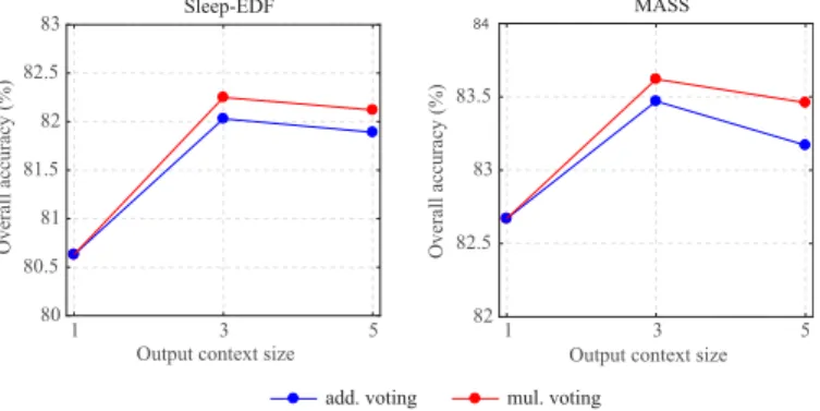
D. The Trade-off Problem with the Output Context Size It is straightforward to extend the output context in the proposed framework. Doing so, we are able to increase the number of decisions in an ensemble, which is expected to en-hance the classification performance [39]. However, extending the output context confronts us with a trade-off problem. A large context weakens the link between the input epoch and the far-away neighbors in the output context. Oftentimes, this deteriorates the prediction decisions on these epochs and, as a consequence, reduces the quality of individual decisions in the ensemble. The low quality of these prediction decisions may
outweigh the benefits of the increased cardinality, worsening the performance instead collectively.
To support our argument, we increased the output context
size to 5 (i.e. τ = 2) and repeated the experiment in which
we set Q = 1000 for the 1-max CNN and used P = 2 for
Sleep-EDF andP = 3for MASS. Figure 8 shows the obtained
performance alongside those obtained with the output context size of {1, 3} (i.e. τ = {0,1}). Note that, with the context size of 1, the framework is reduced to the one-to-one baseline
framework described in Section V-C. With the context size of5
the proposed framework still maintains its superiority over the standard classification setup, however, a graceful degradation compared to the context size of3can be observed. Specifically, the accuracy rates obtained by both additive and multiplicative
voting schemes slightly decline by0.1%on Sleep-EDF while
the respective accuracy losses of0.3%and0.2%can be seen on MASS.
To remedy the weak links between the input epoch and far-away epochs, one possibility is to combine multiple epochs into the input to form the contextual input. In addition, it would be worth exploring incorporation of long-term context (i.e. in order of dozens of epochs), for example using RNNs as in [17], [22]. However, a detailed study of the proposed frame work in these many-to-many settings is out of the scope of this article and is left for future work.
E. Multitask vs Ensemble
To examine the comparability between the proposed mul-titask framework with its ensemble equivalence, we repeated the experiments with the ensemble consisting of three separate CNNs for individual subtasks: left prediction, classification, and right prediction. We studied both the 1-max CNN and the
deep CNN baseline here. Again, we setQ= 1000, andP = 2
for Sleep-EDF and P = 3for MASS when 1-max CNN was
used. The results obtained with the ensemble models and the proposed multitask models are contrastedvis-`a-visin Figure 9. Our analyses show that the separate CNNs of an ensemble model perform better than its corresponding multitask model on the individual subtasks. This is due to the fact that the multitask model needs to deal with a harder modelling task which combines all the subtasks as a whole. However, after aggregation, their differences become negligible as can be seen over all CNN architectures and datasets. More importantly, on both datasets, the proposed multitask 1-max CNN outperforms the deep CNN baseline in its both forms, namely multitask and ensemble.
VII. CONCLUSIONS
This work introduced a joint classification and prediction formulation wherein a multi-task CNN framework is proposed for automatic sleep staging. Motivated by the dependency nature of sleep epochs, the framework’s purpose is to jointly perform classification of an input epoch and prediction of the labels of its neighbors in the context output. While being orthogonal to the widely adopted many-to-one classification scheme relying on contextual input, we argued that the pro-posed framework avoids the shortcomings experienced by the
Output context size 80 80.5 81 81.5 82 82.5 83 Sleep-EDF
Output context size 82 82.5 83 83.5 84 MASS 1 3 5 1 3 5
add. voting mul. voting
Overall accuracy (%)
Overall accuracy (%)
Figure 8: Influence of the output context size to the overall accuracy of the proposed framework. The results obtained with
a common Q = 1000, in addition,P = 2 (Sleep-EDF) and
P = 3(MASS). 70 72 74 76 78 80 82 Overall accuracy (%)
1-max CNN Deep CNN baseline
76 78 80 82 84 Sleep-EDF MASS
1-max CNN Deep CNN baseline
Ensemble Multitask mul. voting add. voting right prediction classification left prediction
Figure 9: Performance comparison of the proposed multitask 1-max CNN with its equivalent ensemble model. The results
are obtained with Q = 1000, P = 2 with Sleep-EDF and
P = 3for MASS.
many-to-one approach, such as the inherent modelling ambi-guity and the induced computational overhead due to large contextual input. More importantly, due to multitasking, the framework is able to conveniently produce multiple decisions on a certain epoch thereby forming the reliable final decision via aggregation. We demonstrated the generalizability of the framework on two public datasets, Sleep-EDF and MASS.
ACKNOWLEDGMENT
The research was supported by the NIHR Oxford Biomed-ical Research Centre and Wellcome Trust under Grant 098461/Z/12/Z.
REFERENCES
[1] A. C. Krieger, Ed.,Social and Economic Dimensions of Sleep Disorders, An Issue of Sleep Medicine Clinics. Elsevier, 2017.
[2] S. J. Redmond and C. Heneghan, “Cardiorespiratory-based sleep staging in subjects with obstructive sleep apnea,” IEEE Trans. Biomedical Engineering, vol. 53, pp. 485–496, 2006.
[3] K. A. I. Aboalayonet al., “Sleep stage classification using EEG signal analysis: A comprehensive survey and new investigation,” Entropy, vol. 18, no. 9, p. 272, 2016.
[4] J. M. Kelly, R. E. Strecker, and M. T. Bianchi, “Recent developments in home sleep-monitoring devices,”ISRN Neurology, vol. 2012, 2012. [5] A. Krakovsk´a and K. Mezeiov´a, “Automatic sleep scoring: A search for
an optimal combination of measures,”Artificial Intelligence in Medicine, vol. 53, no. 1, pp. 25–33, 2011.
[6] B. Koley and D. Dey, “An ensemble system for automatic sleep stage classification using single channel EEG signal,”Computers in Biology and Medicine, vol. 42, no. 12, pp. 1186–95, 2012.
[7] H. Phanet al., “Metric learning for automatic sleep stage classification,” inProc. EMBC, 2013, pp. 5025–5028.
[8] K. Susmakova and A. Krakovska, “Discrimination ability of individual measures used in sleep stages classification,”Artificial Intelligence in Medicine, vol. 44, pp. 261–277, 2008.
[9] J. Fell et al., “Discrimination of sleep stages: a comparison between spectral and nonlinear eeg measures,” Electroencephalography and Clinical Neurophysiology, vol. 98, no. 5, pp. 401–10, 1996.
[10] D. J. Kimet al., “An estimation of the first positive Lyapunov exponent of the EEG in patients with schizophrenia,”Psychiatry Research, vol. 98, no. 3, pp. 177–89, 2000.
[11] J. M. Lee et al., “Detrended fluctuation analysis of EEG in sleep apnea using MIT/BIH polysomnography data,”Computers in Biology and Medicine, vol. 32, pp. 37–47, 2012.
[12] X.-S. Zhang, R. J. Roy, and E. W. Jensen, “EEG complexity as a measure of depth of anesthesia for patients,”IEEE Trans. Biomedical Engineering, vol. 48, no. 12, pp. 1424–1433, 2001.
[13] E. Alickovic and A. Subasi, “Ensemble SVM method for automatic sleep stage classification,”IEEE Trans. Instrum. Meas, 2018.
[14] P. Memar and F. Faradji, “A novel multi-class EEG-based sleep stage classification system,”IEEE Trans. Neural Systems and Rehabilitation Engineering, vol. 6, no. 1, pp. 84–95, 2018.
[15] R. Boostania, F. Karimzadeha, and M. Nami, “A comparative review on sleep stage classification methods in patients and healthy individuals,” Comput. Methods Programs Biomed., pp. 77–91, 2017.
[16] S. A. Imtiaz and E. Rodriguez-Villegas, “Automatic sleep staging using state machine-controlled decision trees,” inProc. EMBC, 2015. [17] J. B. Stephansenet al., “The use of neural networks in the analysis of
sleep stages and the diagnosis of narcolepsy,”arXiv:1710.02094, 2017. [18] K. Mikkelsen and M. De Vos, “Personalizing deep learning models for
automatic sleep staging,”arXiv:1801.02645, 2018.
[19] J. Zhang and Y. Wu, “A new method for automatic sleep stage classifi-cation,”IEEE Trans. on Biomedical Circuits and Systems, vol. 11, no. 5, pp. 1097–1110, 2017.
[20] O. Tsinaliset al., “Automatic sleep stage scoring with single-channel EEG using convolutional neural networks,”arXiv:1610.01683, 2016. [21] O. Tsinalis, P. M. Matthews, and Y. Guo, “Automatic sleep stage scoring
using time-frequency analysis and stacked sparse autoencoders,”Annals of Biomedical Engineering, vol. 44, no. 5, pp. 1587–1597, 2016. [22] A. Supratak et al., “Deepsleepnet: A model for automatic sleep stage
scoring based on raw single-channel eeg,”IEEE Trans. Neural Syst. Rehabil. Eng., vol. 25, no. 11, pp. 1998–2008, 2017.
[23] H. Dong et al., “Mixed neural network approach for temporal sleep stage classification,”IEEE Trans. Neural Syst. Rehabil. Eng., 2017. [24] H. Phanet al., “DNN filter bank improves 1-max pooling cnn for
single-channel EEG automatic sleep stage classification,” inProc. EMBC, 2018. [25] H. Phanet al., “Automatic sleep stage classification using single-channel EEG: Learning sequential features with attention-based recurrent neural networks,” inProc. EMBC, 2018.
[26] Y. LeCun, Y. Bengio, and G. Hinton, “Deep learning,”Nature, vol. 521, pp. 436–444, 2015.
[27] Y. Lecun,Connectionism in perspective. Elsevier, 1989, ch. General-ization and network design strategies.
[28] M. L¨angkvist, L. Karlsson, and A. Loutfi, “Sleep stage classification using unsupervised feature learning,” Advances in Artificial Neural Systems, vol. 2012, pp. 1–9, 2012.
[29] S. Hochreiter and J. Schmidhuber, “Long short-term memory,”Neural Comput., vol. 9, no. 8, pp. 1735–1780, 1997.
[30] P. Kochet al., “Recurrent neural network based early prediction of future hand movements,” inProc. EMBC, 2018.
[31] P. Kochet al., “Recurrent neural networks with weighting loss for early prediction of hand movements,” inProc. EUSIPCO, 2018.
[32] A. H. Ansariet al., “Neonatal seizure detection using deep convolutional neural networks,”International Journal of Neural Systems, vol. 28, p. 1850011, 2018.
[33] C. Iberet al., “The AASM manual for the scoring of sleep and associ-ated events: Rules, terminology and technical specifications,”American Academy of Sleep Medicine, 2007.
[34] S.-F. Liang et al., “A rule-based automatic sleep staging method,” in Proc. EBMC, 2011, pp. 6067–6070.
[35] T. Sousaet al., “A two-step automatic sleep stage classification method with dubious range detection,” Computers in Biology and Medicine, vol. 59, pp. 42–53, 2015.
[36] C. O’Reillyet al., “Montreal archive of sleep studies: An open-access resource for instrument benchmarking & exploratory research,”Journal of Sleep Research, pp. 628–635, 2014.
[37] S. Chambon et al., “A deep learning architecture for temporal sleep stage classification using multivariate and multimodal time series,”IEEE Trans. on Neural Systems and Rehabilitation Engineering, vol. 26, no. 4, pp. 758–769, 2018.
[38] F. Andreottiet al., “Multichannel sleep stage classification and transfer learning using convolutional neural networks,” inProc. EMBC, 2018. [39] G. Hinton, O. Vinyals, and J. Dean, “Distilling the knowledge in a neural
network,”arXiv:1503.02531, 2015.
[40] T. G. Dietterich, Multiple classifier systems. Springer, 2000, ch. Ensemble methods in machine learning, pp. 1–15.
[41] A. R. Hassan and M. I. H. Bhuiyan, “Automatic sleep scoring using sta-tistical features in the EMD domain and ensemble methods,”Biocybern. Biomed. Eng., vol. 36, no. 1, pp. 248–255, 2016.
[42] B. Kempet al., “Analysis of a sleep-dependent neuronal feedback loop: the slow-wave microcontinuity of the EEG,”IEEE Trans. on Biomedical Engineering, vol. 47, no. 9, pp. 1185–1194, 2000.
[43] A. L. Goldbergeret al., “Physiobank, physiotoolkit, and physionet: Com-ponents of a new research resource for complex physiologic signals,” Circulation, vol. 101, pp. e215–e220, 2000.
[44] J. A. Hobson, “A manual of standardized terminology, techniques and scoring system for sleep stages of human subjects,” Electroencephalog-raphy and Clinical Neurophysiology, vol. 26, no. 6, p. 644, 1969. [45] S. A. Imtiaz and E. Rodriguez-Villegas, “Recommendations for
per-formance assessment of automatic sleep staging algorithms,” in Proc. EMBC, 2014, pp. 5044–5047.
[46] S. A. Imtiaz and E. Rodriguez-Villegas, “An open-source toolbox for standardized use of PhysioNet Sleep EDF Expanded Database,” inProc. EMBC, 2015, pp. 6014–6017.
[47] H. Phanet al., “Improved audio scene classification based on label-tree embeddings and convolutional neural networks,”IEEE/ACM Trans. on Audio, Speech, and Language Processing, vol. 25, no. 6, pp. 1278–1290, 2017.
[48] H. Phanet al., “Robust audio event recognition with 1-max pooling convolutional neural networks,” in Proc. INTERSPEECH, 2016, pp. 3653–3657.
[49] Y. Kim, “Convolutional neural networks for sentence classification,” in Proc. EMNLP, 2014, pp. 1746–1751.
[50] V. Nair and G. E. Hinton, “Rectified linear units improve restricted boltzmann machine,” inProc. ICML 2010, 2010, pp. 807–81. [51] N. Srivastavaet al., “Dropout: A simple way to prevent neural networks
from overfitting,” Journal of Machine Learning Research (JMLR), vol. 15, pp. 1929–1958, 2014.
[52] D. P. Kingma and J. L. Ba, “Adam: a method for stochastic optimiza-tion,” inProc. ICLR, no. 1—13, 2015.
[53] H. Phanet al., “Audio scene classification with deep recurrent neural networks,” inProc. INTERSPEECH, 2017, pp. 3043–3047.
[54] M. Abadiet al., “Tensorflow: Large-scale machine learning on hetero-geneous distributed systems,”arXiv:1603.04467, 2016.
[55] S. I. Dimitriadis, C. Salis, and D. Linden, “A novel, fast and efficient single-sensor automatic sleep-stage classification based on complemen-tary cross-frequency coupling estimates,”Clinical Neurophysiology, vol. 129, no. 4, pp. 815–828, 2018.
[56] T. H. Sanders, M. McCurry, and M. A. Clements, “Sleep stage classifi-cation with cross frequency coupling,” inProc. EMBC, 2014. [57] A. M. Munket al., “Semi-supervised sleep-stage scoring based on single
channel EEG,” inProc. ICASSP, 2018, pp. 2551–2555.
[58] J. L. Rodr´ıguez-Soteloet al., “Automatic sleep stages classification using eeg entropy features and unsupervised pattern analysis techniques,” Entropy, vol. 16, no. 12, pp. 6573–6589, 2014.
[59] H. Phan et al., “Weighted and multi-task loss for rare audio event detection,” inProc. ICASSP, 2018, pp. 336–340.
[60] R. S. Rosenberg and S. Van Hout, “The american academy of sleep medicine inter-scorer reliability program: Respiratory events,” Journal of Clinical Sleep Medicine, vol. 10, pp. 447–454, 2014.
[61] C.-E. Kuo and S.-F. Liang, “Automatic stage scoring of single-channel sleep EEG based on multiscale permutation entropy,” inProc. BioCAS, 2011, pp. 448–451.
[62] T. Lajnefet al., “Learning machines and sleeping brains: Automatic sleep stage classification using decision-tree multi-class support vector machines,”J. Neurosci. Methods, vol. 250, pp. 94–105, 2015. [63] C. S. Huang et al., “Knowledge-based identification of sleep stages
based on two forehead electroencephalogram channels,” Frontiers in Neuroscience, vol. 8, p. 263, 2014.
![Figure 4: Ensemble of decisions available at the epoch index n made by the epochs X i in the neighborhood [n − τ, n + τ ], i.e](https://thumb-us.123doks.com/thumbv2/123dok_us/778154.2598410/6.918.146.769.83.234/figure-ensemble-decisions-available-epoch-index-epochs-neighborhood.webp)

![Figure 7: Hypnogram of one subject of the MASS dataset (subject 22 of the subset SS1 [36]): (a) ground-truth, (b) the one-to- one-to-one baseline framework’s output, (c) the many-to-one-to-one baseline framework’s output, (d) the proposed one-to-one-to-man](https://thumb-us.123doks.com/thumbv2/123dok_us/778154.2598410/11.918.131.788.81.383/figure-hypnogram-subject-baseline-framework-baseline-framework-proposed.webp)