Univerzita Karlova v Praze
Fakulta sociálních v
ě
d
Institut ekonomických studií
Rigorózní práce
Univerzita Karlova v Praze
Fakulta sociálních v
ě
d
Institut ekonomických studií
Rigorózní práce
Is the Concept of the Laffer Curve Valid ?
The Empirical Evidence from the Corporate Income Tax for Selected
OECD Countries
Author: Karel Herbst
Supervisor: Doc. MPhil. Ond
ř
ej Schneider, Ph.D., McKinsey Chair
September 2008
Hereby I claim that I elaborated this thesis on my own, and that the only literature and sources I used are those listed in references.
15th of September 2008 author’s signature
Prohlášení
Prohlašuji, že jsem tuto rigorózní práci vypracoval samostatně a použil pouze uvedené prameny a literaturu.
Acknowledgments
First and foremost I would like to thank to my supervisor Doc. MPhil. Ondřej Schneider, Ph.D., for his patience, valuable comments, suggestions and support, while I was writing this thesis.
In addition I would like to thank to my collegue Mgr. Ondřej Strecker for the fruitful consultations concerning the use of econometric techniques.
I am indebted to Professor Joel B. Slemrod, Professor James R. Hines Jr. from University of Michigan and to Mgr. Tomáš Holub, Ph.D. from Czech National Bank (CNB) for informing me about various data sources for my analysis.
Lastly, I would like to thank to my family and to Anna for their patience.
Abstract
This thesis deals with the issue of Laffer curve. According to the idea of the Laffer curve when the tax rate exceeds certain treshold (revenue-maximizing tax rate) the tax revenue would in absolute terms decrease with rising tax rate. Therefore this thesis tries to discover whether those facts are valid in the corporate income taxation for 20 OECD countries for the time period from 1965 to 2006.
The structure of the thesis could be divided into three parts. In first introductory chapters the issue of taxation would be discussed in general. It will briefly examine the history of taxation and explore the theory of taxation and tax systems. The second part of this thesis will focus on the Laffer curve in detail. Third chapter will introduce the theory behind Laffer curve and discuss its properties for different types of taxation. In the following chapter the literature and different possibilities of estimation of the Laffer curve and (or) Laffer effects would be reviewed. Fifth chapter focuses on the corporate income taxation per se and examines the development of corporate income tax revenue and rates in our sample countries.
In the last part of this thesis the econometric estimates of the Laffer curve for corporate income taxation are presented. The Laffer curve would be estimated for three selected countries and then for the whole sample of 20 OECD countries on the panel data. Last section then states conclusions of this thesis, mainly that the Laffer effects for corporate income taxation were confirmed and thus the traditional shape of the Laffer curve was validated.
JEL Classification: H25, H87
Keywords: Laffer curve, Laffer effects, corporate income taxation, corporate income tax revenue
Abstrakt
Tato rigorózní práce se zabývá Lafferovou křivkou. Teorie Lafferovy křivky nám říká, že pokud výše daňové sazby překročí určitou mez (daňová sazba maximalizující příjmy), tak daňové výnosy budou dále v absolutních číslech klesat se vzrůstající daňovou sazbou. Proto se tato práce snaží zjistit, zda jsou tyto skutečnosti platné pro daň z příjmu korporací pro 20 OECD zemí v časovém období od roku 1965 do 2006.
Struktura práce může být rozdělena do tří částí. V prvních dvou úvodních kapitolách bude krátce diskutována historie a teorie zdanění a daňových systémů. Druhá část práce se zaměří na Lafferovu křivku. Třetí kapitola prozkoumá teorii Lafferovy křivky a bude diskutovat její vlastnosti pro různé druhy daní. V následující kapitole je zhodnocena literatura týkající se možných způsobů odhadů této křivky a Lafferových efektů. Pátá kapitola se pak zaměřuje na korporátní daň z příjmu a zkoumá vývoj daňových sazeb a státních výnosů v našem vzorku zemí.
V poslední části této práce jsou prezentovány ekonometrické odhady Lafferovy křivky pro daň z příjmu korporací. Nejdříve je Lafferova křivka odhadnuta pro tři vybrané země a poté pro celý vzorek 20 OECD zemí na základě panelových dat. Závěrečná sekce poté činí závěry z naší analýzy, především potvrzuje, že tradiční tvar Lafferovy křivky pro korporátní daň
z příjmu byl ověřen.
JEL Klasifikace: H25, H87
Klíčová slova: Lafferova křivka, Lafferovy efekty, daň z příjmu korporací, státní výnosy z daně z příjmu korporací
Contents
LIST OF TABLES AND FIGURES... 1
LIST OF ABBREVIATIONS... 2
INTRODUCTION... 3
1 A BRIEF HISTORY OF TAXATION ... 5
1.1 ANCIENT PERIOD... 5
1.1.A Ancient Rome... 5
1.2 TAXATION IN THE MIDDLE AGES... 6
1.2.A Taxation System in the Cities ... 7
1.3 PRE-MODERN PERIOD... 8
1.3.A Introduction of Income Taxes... 8
1.3.B Growing State Expenditures... 8
1.4 MODERN PERIOD... 9
1.4.A Reasons of Rapid Increase of the Public Sector in the 20th Century ... 10
1.4.B The Development after the World War Two... 11
1.4.C Total Tax Revenue in Different Countries... 11
1.4.D Closing Remarks ... 12
2 INTRODUCTION TO THE THEORY OF TAXATION AND TAX SYSTEMS .. 14
2.1 DIFFERENT THEORIES OF TAXATION... 14
2.1.A The Benefit Theory ... 14
2.1.B Ability to Pay Theory... 15
2.2 THE RATIONALE FOR STATE INTERVENTION... 15
2.2.A Roles of Government ... 15
2.2.B Market Failures – Rationale for Government Activity... 16
2.2.C Another State Interventions... 17
2.3 THE SIZE OF THE GOVERNMENT... 17
2.3.A Income Effect and Wagner’s Law ... 19
2.3.B Baumol Effect ... 22
2.3.C Median Voter Theory ... 24
2.3.D Other Factors Influencing the Size of the Government... 26
2.4 PROPERTIES OF TAX SYSTEMS AND THEIR EFFICIENCY... 27
2.4.A Optimal Taxation... 29
2.4.B Efficient Tax Systems... 30
2.4.C Concluding Remarks ... 31
3 LAFFER CURVE THEORY ... 33
3.1 THE THEORY BEHIND THE LAFFER CURVE... 33
3.1.A Review of Thoughts ... 33
3.1.B The Theory... 35
3.1.C Laffer Curve for Different Taxes... 36
3.1.D Mathematic Rationale ... 38
3.1.E Revenue-Maximizing Tax Rate... 38
3.1.F Supply-Side Economics ... 39
3.2 THOUGHTS ON THE LAFFER CURVE... 39
3.2.A Shifty Laffer Curve ... 40
3.2.B Multiple Peaks of the Laffer Curve ... 42
3.2.D Concluding Remarks ... 44
4 REVIEW OF LITERATURE CONCERNING THE LAFFER CURVE ESTIMATION... 45
4.1 ESTIMATIONS BASED ON EQUILIBRIUM MODELS... 45
4.1.A Static Models ... 46
4.1.B Country Specific Estimates... 47
4.1.C Dynamic Models... 48
4.1.D Estimation of Laffer Effects without Deriving the Laffer Curve ... 50
4.2 OTHER TYPES OF ESTIMATIONS... 51
4.2.A Estimates based on Tax Evasion ... 51
4.2.B Economic Experiments... 52
4.3 SOLELY ECONOMETRIC ESTIMATIONS OF LAFFER EFFECTS... 53
4.3.A Personal Income Tax Estimation ... 54
4.3.B Corporate Income Tax Estimations... 54
4.4 CONCLUDING REMARKS... 55
5 CORPORATE TAX RATES, REVENUE AND POSSIBLE LAFFER EFFECTS 56 5.1 DEVELOPMENT OF CORPORATE INCOME TAX RATES... 56
5.1.A Tax Competition as an Explanation ... 58
5.1.B Different Explanation... 60
5.2 DEVELOPMENT OF CORPORATE TAX REVENUE... 60
5.3 THE DETERMINANTS OF CORPORATE TAX REVENUE... 62
5.3.A Direct Effect Influencing the Tax Base ... 63
5.3.B Indirect Effects Influencing the Tax Base ... 63
5.3.C Factors of Laffer Effects... 63
5.3.D Non-Laffer Factors... 66
6 TIME–SERIES MODELS FOR THREE SELECTED COUNTRIES ... 67
6.1 BENCHMARK MODEL... 67
6.1.A Description of Variables ... 68
6.1.B The Structure of the Model... 68
6.1.C Other Factors Influencing the Size of Revenue and Their Possible Inclusion into the Model... 69
6.1.D Data Range and Sources ... 70
6.1.E The Existence of Laffer Curve and the Revenue-maximizing Tax Rate ... 70
6.1.F The Issue of Stationarity... 71
6.1.G Limitations of the Chosen Model ... 72
6.2 IRELAND... 73
6.2.A Benchmark model... 74
6.2.B Adjusted Model... 75
6.2.C The Properties of Adjusted Model... 77
6.2.D Economic Explanation of Added Variables ... 78
6.3 FRANCE... 79
6.3.A Benchmark model... 80
6.3.B Adjusted Model... 81
6.3.C The Properties of Adjusted Model... 83
6.3.D Economic Meaning of Adjusted Model ... 83
6.4 UNITED KINGDOM... 84
6.4.A Adjusted Model... 85
6.4.C Country-Specific Results ... 86
6.4.D Concluding Remarks ... 87
7 PANEL DATA MODEL FOR 20 OECD COUNTRIES ... 89
7.1 SELECTED COUNTRIES AND DATA DESCRIPTION... 89
7.2 BENCHMARK MODEL... 90
7.2.A Fixed Effects or Simple Pooled OLS method ? ... 91
7.3 ADJUSTED MODEL... 92
7.3.A Lagged Tax Rates ... 94
7.3.B Estimations for Different Time Periods ... 95
7.3.C Concluding Remarks ... 97
CONCLUSIONS ... 98
REFERENCES... 100
List of Tables and Figures
TABLE 1.1:TOTAL TAX REVENUE IN CHOSEN OECDCOUNTRIES... 12
FIGURE 2.1:TOTAL TAX REVENUE AS % OF GDP... 18
FIGURE 2.2:INCOME TAXES REVENUE AS % OF GDP ... 28
FIGURE 2.3:CONSUMPTION TAXES REVENUE AS % OF GDP... 28
FIGURE 3.1:THE LAFFER CURVE... 36
FIGURE 3.2:DERIVATION OF THE LAFFER CURVE FOR INDIRECT TAXATION... 37
FIGURE 3.3:SHIFTY LAFFER CURVE... 41
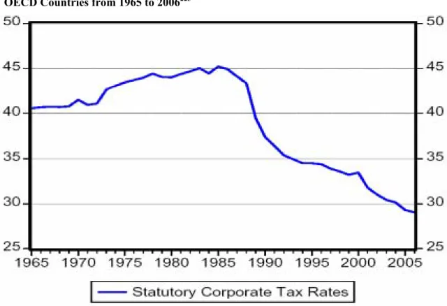
FIGURE 5.1:DEVELOPMENT OF AVERAGE STATUTORY CORPORATION INCOME TAX RATE IN 20 OECDCOUNTRIES FROM 1965 TO 2006... 57
FIGURE 5.2:CORPORATE INCOME TAX RATES FOR SELECTED YEARS (IN %) ... 58
FIGURE 5.3:DEVELOPMENT OF AVERAGE CORPORATE INCOME TAX REVENUE TO GDP( IN %) IN 20 OECDCOUNTIRES FROM 1965 TO 2006 ... 61
FIGURE 5.4:CORPORATE INCOME TAX REVENUE FOR SELECTED YEARS (AS % OF GDP) ... 62
FIGURE 6.1:TAX RATES AND TAX REVENUE IN IRELAND... 74
TABLE 6.1:OLSESTIMATION OF BENCHAMRK MODEL... 75
FIGURE 6.2:REPRESENTATION OF BENCHMARK MODEL... 76
TABLE 6.2:OLSESTIMATION OF ADJUSTED MODEL FOR IRELAND... 77
FIGURE 6.3:TAX RATES AND TAX REVENUE IN FRANCE... 80
TABLE 6.3:OLSESTIMATION OF BENCHMARK MODEL FOR FRANCE... 80
TABLE 6.4:OLSESTIMATION OF ADJUSTED MODEL FOR FRANCE... 82
FIGURE 6.4:REPRESENTATION OF ADJUSTED MODEL FOR FRANCE... 82
FIGURE 6.5:TAX RATES AND TAX REVENUE IN THE UNITED KINGDOM... 84
TABLE 6.5:OLSESTIMATION OF ADJUSTED MODEL FOR UK... 85
FIGURE 6.6:ESTIMATED LAFFER CURVES FOR FRANCE AND UK ... 87
TABLE 7.1:ESTIMATION OF BENCHMARK PANEL DATA MODEL... 91
TABLE 7.2:ESTIMATION OF ADJUSTED PANEL DATA MODEL... 92
TABLE 7.3:ESTIMATION OF ADJUSTED PANEL DATA MODEL WITHOUT NORWAY... 93
TABLE 7.4:ESTIMATION OF ADJUSTED PANEL DATA MODEL FOR LAGGED TAX RATES... 94
TABLE 7.5:ESTIMATION OF ADJUSTED PANEL DATA MODEL FOR TIME SUBSAMPLES... 95
List of Abbreviations
ADF - Augmented Dickey Fuller testDW – Durbin Watson stats. EC - European Communities EU - European Union
GDP – Gross Domestic Product JB – Jarque-Bera test
OECD – Organization for Economic Cooperation and Development OLS-Ordinary Least Squares
VAT – Value Added Tax WW2 – World War Two U.S. – United States
Introduction
It has been said that the virtue of the Laffer curve is that you can explain it to a congressman in half an hour and he can talk about it for six months.
Hal Varian (Intermediate Microeconomics) This thesis will deal with the issue of Laffer curve. As the quotation suggests the concept of this curve and the theory behind is fairly simple. The basic idea lies in the fact that the tax revenue depend on the tax rates, however the dependence is not linear. According to the idea of Laffer curve when the tax rate exceeds certain treshold (revenue-maximizing tax rate) the tax revenue eventually decrease with rising tax rate. More detailed explanation would be given further in the text. We would thus explore whether this concept is valid for corporate income taxation and whether we can estimate the Laffer curve for selected OECD (Organization for Economic Cooperation and Development) countries.
We can divide the structure of the thesis into three parts. In first introductory chapters we would discuss the issue of taxation in general. We will briefly examine the history of taxation and explore the theory of taxation and tax systems. The main emphasis would be devoted to the size of the state sector. This analysis would show us that the state sector grew significantly in last century and therefore there were growing requirements for the funds to finance the state activities. Thus it is legitimate to investigate whether further increase in taxes would constitute the increase of revenue or not.
In the second part of the thesis we focus on the Laffer curve in detail. Third chapter will introduce the theory behind Laffer curve and discuss its properties. In the following chapter we would review the literature and different possibilities of estimation of the Laffer curve and (or) Laffer effects. Fifth chapter serve as a bridge between the second and third part of this thesis. It focuses on the corporate income taxation and we would examine the development and its possible explanations for corporate income tax revenue and rates in sample of 20 OECD countries for the time period from 1965 to 2006.
Last two chapters estimate the Laffer curve for corporate income taxation using the econometric models. In chapter six we try to estimate the Laffer curve for three selected countries (Ireland, France and the United Kingdom) using the time-series estimation technique. In the final chapter the Laffer curve will be estimated for the whole sample of 20 OECD countries on the panel data. Last section then concludes.
Before we proceed, we can state two hypothesis about the estimations of Laffer curve. We would hypothesize that Laffer effects will be significant for corporate income taxation and thus the standard shape of the Laffer curve would be confirmed by our estimates. Moreover, we suppose that there are certain differences in the tax systems and tax revenue collection among OECD countries and thus the results would differ for different countries. This hypothesis is also one of the reasons why we included the country-specific estimates into our analysis in chapter six. Let us now shortly review the history of taxation in the first chapter.
1
A Brief History of Taxation
This passage is rather an overview of some important aspects in the history of taxation and therefore it is not a comperhensive summary. It also focuses mainly on the western countries such as European countries and to some extend the United States (U.S.). The history of taxation goes far back to the ancient times and is highly connected to the development of states.
1.1
Ancient Period
The first known system of taxation was discovered in Ancient Egypt around 3000 BC - 2800 BC in the first dynasty of the Old Kingdom. Administrative texts, literary texts, letters and scenes from tombs have provided evidence that the taxes and tax collectors were present at that time. The pharaoh would then conduct a bienneial royal tour around the country and the inhabitans of Egypt and thus he collected taxes.1
The early taxation is also mentioned in the Bible:
But when the crop comes in, give a fifth of it to Pharaoh. The other four-fifths you may keep as seed for the fields and as food for yourselves and your households and your children.2
However taxes did not play the major role in the ancient world. The purpose of the taxation was mainly to finance military forces, public buildings and administration of the given territory. The tax collection was mainly irregular and especially the in-kind and corvée taxation were typical for the ancient era.3
1.1.A Ancient Rome
As an example we can take one of the greatest empire of that era - Ancient Rome and examine its system of taxation little closer.4 Roman empire relied on the tribute from
state-owned resources. The second source of the state income was the tax collection. Apart from military purposes and public administration the expenditures of the Roman empire went
1 In University of Pennsylvania (2002).
2 In Holy Bible – New International Vesion (1978) chapter 47, verse 24. 3 In Urbášková (1998).
for the entertainment, the city of Rome’s grain supply and salaries of civil servants. The system of taxation in Ancient Rome consisted of three main taxes.
There was a poll tax5 on adults between the age of 12 to 65. This tax was imposed on males or on all adults depending upon the province. However, the largest revenue came from the property tax. It was a fixed amount and therefore it did not vary with the size of the crop.
Another important tax was the harbor tax, which would have been called customs duties in the present days. The rate was set between 2 – 2.5 % of the value of goods imported into the empire. The remarkable exception were the luxury goods imported from eastern provinces which faced 25 % import duty. This rather high rate was set for two purposes. It should have discouraged the outflow of the currency from Rome and obtain the revenue from wealthy Romans. Their demand for the luxury goods was highly inelastic and therefore their willingness to buy those goods did not decrease much even with that high tax rate.6
This system of taxation and state policies led to the situation where Romans residing in Italy benefited. They were responsible for paying only the miscellaneous taxes, however they enjoyed the most fruits of state redistribution. They enjoyed the benefits of protection, public services and free grain (inhabitants of Rome) and all this was financed primarily by the provinces.7
Thanks to the previous short excursion to the system of ancient taxation, it is apparent that the redistribution role of taxation played significant function. It is also obvious that it was not always the redistribution from rich to poor, rather it depended on the place where the inhabitants of the Roman empire were settled.
1.2
Taxation in the Middle Ages
In different territories different state systems and thus different tax systems were evolving during that time, however we could observe some similarities in the forms of taxation which were collected. The following section shortly summarize these similarities.
The most important resource and factor of production in the feudal system was land. Therefore its ownership was the key factor which was subject to taxation. The original owner of the land was the monarch. He either administered the land by his own vassals or he gave
5 See page 29 for explanation of this term. 6 In Angresano (1995), pp. 40-47.
the land to the barons or to the Church8 or he might have lent the land to the vassals or peasants. Therefore land was either publicly owned (by the monarch), owned by the Church, by private individuals (such as barons, vassals and peasants) or by group acting cooperatively.9
Frequently the tenancy of the land was somehow taxed by the landlords or by the monarch. Another forms of taxation were, inter alia, the mandatory gifts for the emperor, import duties, and every holder of the land10 was obliged to provide either military service or labor in return for the right to til his land.11
1.2.A Taxation System in the Cities
The situation in the cities was rather different than in the feudal manors. As time was flowing, the cities earned major importance in the Middle Ages’ system. The most important factor of production in the cities was apparently the labor. Craftsmen and merchants associated into guilds, which had the eminent privilege from the monarch to manufacture the products and run the business.
With the evolution of cities and monetary system, apart from in-kind and labor taxation, the monetary taxation started to play an important role. Those monetary taxes could have been indirect (paid on transaction of goods) or direct (paid on wealth or on income).12 Many cities have also negotiated some sort of charters (e.g. to brew beer) with the monarch and evidently the cities have paid some sort of tax for this privilege.
Before we proceed to the modern period of our history we could summarize the feudal system of the Middle Ages and its implications for the on-coming period. The public expenditures mainly on evolving professional military forces, administration and judiciary significantly rose.13 Thus the need of taxation was more considerable. That is why the monetary taxes started to play much more important role and the main income of the public budget changed from the feudal in-kind taxes to the monetary taxation of the cities. However, the taxation was still mainly irregular and non-lasting. Consequently, the monarch had to appeal the nobility for the permission to introduce certain tax repeatedly.
8 Obviously this gratuity of the monarch was not disintrested and the monarch required some services in return.
See e.g. Angresano (1995), pp. 63-69 for further details.
9 In Angresano (1995), p. 74.
10 This could have been ordinary peasant or even the duke. 11 In Salanié (2003), p. 2.
12 In Salanié (2003), p. 2., for further discussion see next chapter. 13 In Grúň (2004), p. 38.
1.3
Pre-Modern Period
The modification of the taxation system is a long term process. However, during the 15th and 16th century the taxation system started to gradually function on the basis of regular and periodical revenue.14 Therefore taxes became permanent source of state budget and fiscal policy began to form.
The European countries started to discover new land mainly in Africa and America and they began to derive benefits from their colonial possesions. Also the trade policy of the colonial powers have changed and the emphasis was given on the custom duties, internal (between provincies) as well as external.15 The custom duties thus became the main source of the state budget in the colonial powers. States started to be heavily protective and in accordance with the mercantilism they put emphasis on the foreign trade as the most important policy. Hence, they exported their manufactured goods mainly to their colonies and the custom duties on imports from those countries were set very high in order to collect revenue to the state budget as wel as to protect the domestic market from massive inflow of imports.
1.3.A Introduction of Income Taxes
The Napoleonic wars and the need of countries to finance the growing war expenditures led certain governments to introduce first modern income taxes. In England the tax reform which created this income tax took place in year 1798.16 The indirect taxes and customs duties could have been thus lowered. However, in peace time the income tax was again abolished and in England was re-established by the prime minister Robert Peel in year 1842.17 Other countries followed this suit of England and income tax was introduced in
Prussia, France and after overcoming the constitutional objectives of the Supreme Court this tax was introduced in the United States as well in the beggining of the 20th century.18
1.3.B Growing State Expenditures
The rising expenditures of the state budget were not caused solely by the war expenditures. The state bureaucracy started to influence the life of people in many spheres of
14 Ibid, p. 39.
15 In Salanié (2003), p. 3.
16 See Grúň (2004), p. 47 for details. 17 In Salanié (2003), p. 3.
life. Some domains of private sphere were increasingly influenced by the state sector. We could mention, inter alia, the educational system, social services and even architecture or arts.
The growing state sector had an implication that the taxes itself were not enough to cover the rising expenditures of the state budgets. Therefore, the monarch or the governments had to partialy finance the state expenditures by the credit loans. These loans had different forms (e.g. from commercial banks), but evidently it led to the birth of national debt phenomenon.
We can summarize by saying that the state sector was growing and consequently the state revenue were consolidated in order to ensure the financial resources for the rising requirements of the state budgets. However, more frequently the state revenue from taxes and fees were not able to cover the rising expenditures and states became indebted.
1.4
Modern period
The taxation system was influenced and shaped by the thinkers of that era. Adam Smith, David Ricardo and others19 did support the formation of liberalism and minor state intervention to the process of the economy. The liberal ideas influenced mainly the dominance of the free trade and thus the custom duties were cut rapidly. Therefore there was an attempt to restrcit the tax collection solely for the inside and outside security and for the purposes of law and order.20
Despite of the fact that the liberal ideas were extending, the state sector was rather growing than diminishing. That was due to the fact that mainly the military expenditures were rising (new technologies, management and administration of colonies and discovering of new colonies), also administration and expenditures on police, courts and social benefits were increasing. Further we cannot forget that most of the states were indebted as was explained above and they had to service their debt.21
The tax systems started to be compact and they began to play fundamental role in the economy. Balances of revenue and expenditures of state budgets were annually
19 See e.g. Screpanti & Zamagni (1993), pp. 54-118 for their detailed ideas and for further references. 20 In Grúň (2004), p. 63.
compounded and gradually they became analogous to the state budgets as we know them from the present.
Taxes were already distinguished on direct and indirect. And almost every tax was paid in monetary units. We should mention that the public sector still constituted only less than 10 percent of national income in most of the European countries and even less than 5 percent of national income in the U.S. in the end of 19th century.22
1.4.A Reasons of Rapid Increase of the Public Sector in the 20th Century
In the 20th century the public sector grew rapidly and we should now focus on the reasons of this rapid increase. 23 The first reason is the strong and permanent increase of social expenditures which laid the foundation of the modern welfare state as we know it from most developed countries in present period. The origin of the welfare state dates back to the 1883 to Prussia, when the compulsory health insurance was introduced. Only after six years also the pension system in Prussia was created. Other countries followed this suit mainly in the beggining of the 20th century.24 We could have witnessed also the birth of unemployment benefits in this time period.
Secondly, most of the European countries as well as the U.S. were involved in two main war conflicts in the 20th century. Two world wars did increase the military expenditures dramatically. Even between those two war conflicts the size of public sector did not reduce much.25
In the countries which were directly involved in the war, expenditures on military purposes reached or even passed the half of the national income. Some of these skyrocketing expenditures were financed by borrowing, but most of them were covered by the tax increases. Therefore for example the top marginal rates of income taxes became even confiscatory above 90 percent in the United States and United Kingdom during the World War Two.26 The question which would be address in this thesis is then straightforward – do
these tax increases indeed increase the relevant tax revenue ?
22 In Salanié (2003), p. 3.
23 These reasons are taken from historical and social point of view, for economic explanations of the growth of
the public sector in developed economies in 20th century see next chapter where the economic reasons are
elaborated more precisely.
24 See Salanié (2003), p. 4. for exact dates of introduction of these social welfare benefits in different states. 25 As reasons we can mention the birth of the welfare state in many countries, state funds were also needed for
the reconstruction of destroyed regions and infrastructure etc.
1.4.B The Development after the World War Two
After the Second World War in many countries the state finances were used again for the reconstruction of destroyed areas. Moreover, the social contributions were consolidated, for example the Beveridge Report27 helped to consolidate the welfare contributions in the United Kingdom.
The new tax called value-added tax (VAT) was introduced since 1954 in France. VAT was introduced in the European Communities (EC) in the late 1960’s and it was intended to replace four types of sales or turnover taxes, which existed until then in different European countries.28 This tax constitutes almost 20% of tax collection in the European Union29 in the present.30
As a reaction to the growing budget deficits and “stagflation” in the 1970’s there were introduced fiscal reforms from right-wing governments. In some countries the top marginal rates of personal and corporate income taxes were dramatically reduced in order to support growth.31 In the United States this reduction of top marginal rate fell during several years from 70 percent to 28 percent in year 1986.32 In most of the European countries similar reforms took place, however they were more modest.
1.4.C Total Tax Revenue in Different Countries
In Table 1.1 you can find the development of tax revenue in chosen OECD countries since year 1955 to year 2005. From this table it is evident that the total tax burden varies across the developed countries rather considerably. According to the table there are countries, where the total tax revenue constitute almost one half of the GDP of the country (in Sweden it even exceeds one half). Contrariwise, there are countries where the total tax revenue do not reach one third of the GDP such as United States, Japan or Switzerland.
In the table there is also some evidence on the variation in time. However, we can see that the level of tax revenue was rather stable after the WW2 in many developed countries. In some countries there was rather gradual increase of the tax revenue such as in
27 See e.g. Angresano (1995) pp. 273-276 for detailed description of this report.
28 See e.g. El-Agraa (2007), pp. 282-283 for more detailed description of these sales and turnover taxes
29 The autor is aware of the differences between the EC and European Union (EU). Therefore the distinction is
done in the text and to the terms is reffered usually separately.
30 See e.g. European Commission (2008) for more detailed figures on VAT and its collection.
31 See the discussion concerning the supply-side economics and mentioned references in chapter three. 32 In Salanié (2003), p. 4.
United Kingdom, France or Switzerland. However, in Sweden the tax revenue more than doubled since 1955 and thus they rose rather rapidly up to 51.1% of GDP.
Table 1.1: Total Tax Revenue in Chosen OECD Countries
Total tax revenue as a percentage of GDP in chosen OECD countries
1955 1965 1975 1985 1995 2005 France n.a. 34.5 35.5 42.4 42.9 44.3 United Kingdom 29.7 30.4 35.3 37.7 35 37.2 Germany 30.8 31.6 35.3 37.2 37.2 34.7 Sweden 25.5 35 41.6 47.8 48.1 51.1 Switzerland 19.2 17.5 24.5 26.1 27.8 30 United States 23.6 25 25.6 25.6 27.9 26.8 Japan 17.1 18.3 20.9 27.4 26.9 27.4 OECD-total33 24 25.8 29.7 32.9 35.1 36.2 EU-1533 26 27.8 32.4 37.7 39.2 39.7 Source: OECD (2006) n.a. stands for not available.
1.4.D Closing Remarks
From this short excursion to the history of taxation it seems to be apparent that the legacy of the history has implications into the present. Thanks to the historical development countries do differ in the magnitude of taxes as well as in the structure of their tax systems.
Present development has also important implications for the tax systems. The environmental taxes are already part of the taxation system and their significance would be probably more apparent in the future. There are opinions which support the double dividend hypothesis. This hypothesis claims that the environmental taxation would not only contribute to the better environment but also reduce the costs of tax system.34
We should also mention the globalization of the world’s economy. Therefore, the capital is more mobile and people and firms can vote with their feet.35 According to this theory inhabitans and firms choose in which country to reside according to tax rates and levels of public goods. In theory this is possible, however in the practice there are some limitations and impediments in the migration of people and firms into different countries even within the
33 The unweighted averages were used, the EU 15 area countries are : Austria, Belgium, Denmark, Finland,
France, Germany, Greece, Ireland, Italy, Luxembourg, Netherlands, Portugal, Spain, Sweden and United Kingdom.
34 See e.g. Goulder (1995) or Bovenberg (1999) for the description of different forms of double dividend
hypothesis.
European Union.36 However, even this phenomenon of tax competition37 contributed to the lowering of personal and corporate income taxes and mainly to their top marginal rates. This issue concerning the corporate income taxation would be discussed in greater detail in chapter five.
In the next chapter we will more closely explore different theories of taxation, the rationale for government interventions into the economy and the economic reasons for rather substansive size of the public sector in developed economies. Moreover, we will briefly comment basic properties of tax systems and tax efficiency.
36 As such impediments we can see different laguages, different norms and legal practises and also the fact that
people in Europe do not migrate that much as in the United States.
37 Tax competition is concept where regions or countries compete to attract firms and capital to settle down in
2
Introduction to the Theory of Taxation and Tax
Systems
Taxes and taxation systems are present in the everyday life of all human beings and they affect our decisions concerning work and labor supply, savings, education, consumption, retirement etc. Also on the macroeconomic level taxes affect very broad spectrum of subjects from level and structure of investment to allocation of governmental resources into public goods and other services provided by the government. Tax policy may also reflect the elements of national culture and the values of society other than equity or individualism.
In this section we at first briefly review different theories of taxation, then we will focus on the reasons why the government intervenes and why the magnitude of the public sector is that sizable and varies accross the countries.
2.1
Different Theories of Taxation
During the time there evolved several tax theories which explain the creation and purpose of taxes and we should now investigate them more closely. Two main ones are the benefit theory of taxation and the ability to pay theory and we shortly review them. Among other theories we can classify economic surplus theory38, utilitarism or ideas of Rawls or Nozick,39 however we will not review them here.
2.1.A The Benefit Theory
According to its term this theory argues that each individual should contribute to the state system in accordance with the benefits he derives from the state. Taxes therefore should reflect the demand of individuals for public services (e.g. the protection, health service etc.).
The critiques of this theory claim that it requires to measure values which are hardly measurable and it is incompatible with social justice and fairness.40 Thus this theory could be applied solely to some specific taxes, such as the fuel tax (consumption tax on fuels). The revenue from this tax should be used for developing of the quality of roads and highways,
38 See Trotman-Dickenson (1996), p. 115 for detailed explanation.
39 For detailed description of those theories and ideas as well as for further references see e.g. chapter three in
Barr (2004), pp. 42-63.
transportation services etc. Therefore there is visible link – those who pay the tax also receive benefits from this taxation.41
2.1.B Ability to Pay Theory
This theory is mostly recognized theory of taxation.42 It tackles the problem of equity and social justice and it declares that individuals should contribute to the system according to their means. Hence those in need of state benefits do not have to, according to this theory, contribute to the system heavily.
As an example of the tax which would be explained by this theory we could mention for instance progressive income taxation. The taxpayers with lower income would pay lower taxes and the problem of social justice is therefore settled.43
2.2
The Rationale for State Intervention
We have shortly reviewed theories of taxation which try to explain how the taxation was introduced and who should pay different taxes. Let us now focus on the reasons why taxes are needed and why the public sector engages from one third to over one half of the whole economies of the developed countries as we have seen in the previous section. At first we should focus on the roles of government and then we would investigate when the government (state) should intervene into the market.
2.2.A Roles of Government
According to Musgrave44 the government has three functions on the field of economy45 in the democratic society. With the stabilization function the government should maintain stable prices and employment. This could be done by using the monetary and fiscal policy.
The allocation function should ensure that the goods and services are allocated in sufficient quantities for the consumers. That could be done through the market (state should solely supervise and enforce laws) or via government provisioning
41 See Voorhees (2005), pp. 90-91 for detailed discussion of these examples. 42 See e.g. Trotman-Dickenson (1996), pp. 117-118.
43 See Voorhees (2005), pp. 90-91 for details.
44 Originally in Musgrave (1939), taken from Voorhees (2005) pp. 88-90.
45 Note that these are not functions on the political field. There would evidently be different functions of the
The most discussed and controversial function is the distribution of wealth. The level of redistribution varies greatly among countries and it is highly connected to the notion of fairness and equity.
2.2.B Market Failures – Rationale for Government Activity
According to the two fundamental theorems of welfare economics the market provision of goods is superior than the public provision.46 However the assumptions of those theorems are restrictive and if those assumptions are not satisfied the private market provision is not efficient. We should now focus exactly on those situations, when the market provision is not Pareto-efficient and when the state intervention should be necessary – those conditions, when the governmental activity is rational, are called market failures. Below we only shortly review the most known market failures.47
Several reasons in some industries could cause that there exist relatively few firms with a large share of the market. Therefore there has to be control of abuse of dominant position (regulation, state intervention), since these firms are more liable to that kind of unethical behaviour.
Public Goods are goods with special properties which ensure that their provision by the market would be insufficient or they would not be provided at all. Those properties are non-excludability and non-rivalry in consumption.48 Typical examples which would ensure both of these properties are, inter alia, national defense of a country, lighthouse for ships on the sea or a system of justice.
Situations when the action of individual or a firm affects other individuals or firms and the latter are not compensated for that actions are called externalities (negative or positive). One of the most wide-spread solution to externalities is regulation or imposing penalties and fees (rewarding for positive externalities).
The literature mentions also incomplete markets (e.g. the market for loans and insurance) and information faiures as market failures.
46 See e.g. Stiglitz (2000), pp. 60-61.
47 For more detailed description of market failures and their exercise in practise see e.g. Stiglitz (2000) pp. 76-86. 48 Obviously those properties are usually not satisfied fully, therefore pure public goods are rare in the real
world. Most of the public goods have characteristics of non-rivalry and non-excludability to some degree and they are called impure public goods. See Trogen (2005) pp.169-205 for full characteristics of impure public goods and other specifications such as excludable public good or congestible public good (the assumption of non-rivality is violated).
2.2.C Another State Interventions
The state involvement in the situation of merit goods is based on the assumption that the individual may not act in his own best interest, even if he has all the necesarry information. The typical merit goods where the state involvement urges individuals to consume them are seat belts in the cars or elementary compulsory education.49
Redistribution of income to the needy or we could use the term equity is another situation when the government intervenes and thus uses taxes. There are two types of equity – horizontal and vertical equity. The former one is rather easily accepted and requires that there should be equal treatment of those who are in all relevant aspects the same. These relevant aspects could be understood as gender, age, ethnical or religious conviction etc. In majority of cases this horizontal equity is satisfied across developed countries.
However vertical equity is much more complex and complicated issue which depends mainly on the normative perception to what extend the redistribution should take place. It is essential to claim that the state involvement in such situations is not approved by everyone and it depends on the normative judgements of each individual.
2.3
The Size of the Government
As it was mentined in the previous section, the size of the government grew significantly throughout 20th century in developed and also in most of the developing countries. In Figure 2.1 you can see total tax revenue as a percentage of GDP for OECD countries in years 2000 and 2006. Remeber also the Table 1.1 from previous chapter. Note that on average the size of the public sector which could be approximated by the total tax revenue50 exceeds 35% in OECD countries and it could extend even beyond 50% level.
49 In Stiglitz (2000), p. 87.
50 Evidently this is sort of simplification, since government has certain other tools how to obtain additional
Figure 2.1: Total Tax Revenue as % of GDP
Source: OECD (2008)
Since the previous chapter focused mainly on political and social reasons for the size of the government and its growth in the 20th century we should explore the economic reasons and explanations of such a growth.
The pattern of the growth was evident in the first half of the 20th century and after the World War II, since 1970’s the pattern has been much more varied. Countries as United States, Belgium, Netherlands and Italy experienced decline in the share of government consumption in GDP. On the other hand, Austria, Finland, France, Norway, Portugal and other countries experienced the opposite and the share of government consumption in GDP has grown significantly.51
To explain the size of the government in the developed countries the equation (1) could be used:52
(
1
)
(
1
)
(
1
)(
1
)
( )
1
g
•=
η
+
p
•+
δ
−
y
•+
α
−
η
+
N
•+
δ
k
•+
φ
m
• where the variables with the dots represent the growth rate of the given variable.53The explained variable g is the share of government spending in the agregate real output. Right-hand-side explanatory variables: N stands for population size, p is the relative
51 See Borcherding et al. (2004), pp. 77-79 for detailed describtion of the above mentioned development and for
exact figures or see Table 1.1 in this thesis.
52 It was firstly derived and used in Borcherding (1977). 53 More formally the notation should be x
x
∂
price of government services (to all other goods), y stands for mean income, k is the ratio of median to mean income and m stands for a set of political control variables.
If we take a look on the parametrs, η represents the price elasticity of demand for government consumption, α is the degree of publicness of the output of the government sector,δ represents the income elasticity of demand, φ is the set of elasticities for the effect of the various political controls on demand. This form is useful for estimating and discussing the effects of various variables on the real government size and its growth.54 The vast literature evaluate the effects of those different variables on the size of the government sector and we will discuss those factors in more details.
2.3.A Income Effect and Wagner’s Law
German economist Adolph Wagner, who lived mainly in the 19th century and on the beggining of the 20th century, has investigated the expanding state expenditures and he observed empirical regularities in the growth of public enterprises as individual economies develop. These regularities were not only in the absolute terms but also in the relative portion of the public sector to the whole economy – this relationship is thus called „Wagner’s Law” or “Law of increasing state activity”.55 Thus we could regard the public sector services as some kind of luxury good, where its consumption rise with income of the particular country not only in absolute values but also in reative terms. Thus the income elasticity of demand for government services would be higher than unity.
Wagner believed that the increasing expenditures are associated with traditional state activity such as defense and maintaining law and order as well as with the implementation of newer activities: more emphasis on the education, welfare services and incrasing use of government regulations.56 Wagner stated that the growth of real income would strengthen the relative expansion of income-elastic cultural and welfare expenditures. These areas such as culture and education would be in general more efficiently produced by the public producers than by the private ones.57 Wagner also noted that there has to be upper limit for the proportion of government growth, but he did not specify it exactly.58
54 In Borcherding et al. (2004), p. 80. 55 In Peacock & Scott (2000), pp. 1-2.
56 Originally in Wagner (1911), taken from Peacock & Scott (2000), pp. 2-3. 57 In Henrekson (1993), p. 407.
Review of Literature on Wagner’s Law
There exist a vast literature which investigate the relation of economic development and the growth of public sector (government activities). Therefore we will mention only few of them and study whether these studies confirm Wagner’s Law or reject it. We also have to keep in mind that different authors used different specifications of the model, they used different measures of government59, most of them omit to include public utilities (enterprises)60 and the usage of independent variables also differs among studies. Different problems in the econometric techniques may arise as well and they would be shortly discussed below.
Earlier studies61 do mostly confirm the Wagner’s Law on their chosen samples of
countries and time periods. These studies estimated either
(
δ −1)
term as is specified in the Equation (1). Thus if this elasticity is significantly greater than 0, the hypothesis of Wagner’s Law could be confirmed. Or the studies estimated directly the income elasticity δ in that case if this elasticity is significantly greater than 1, they confirmed Wagner’s Law hypothesis.62Different Problems of Estimations
However, if we have a closer look on these studies which focused on time series rather than cross-section data, we discover that the problem of non-stationarity of the data arises. It means that one of the basic assumption of time-series analysis that all regressors are either deterministic or stationary random variables is violated.63 In most earlier studies that
assumption is not met and thus the standard OLS regression brings inconsistent estimates if the integrated dependent variable is not co-integrated with one of the regressors.64 Therefore those studies which omitted the problem of non-stationarity brought spurious regressions, where there was high level of R2 but very low Durbin-Watson statistics and the estimated coefficient are not efficient.65
59 From very narrow sence excluding transfers and defense expenditures to broad definitions where all
expenditures are included. See Peacock & Scott (2000) p. 5. for the discussion about different inclusion of different definitions of government.
60 See the critical discussion concerning these omissions and why it could have been actually beneficial for the
authors regarding their results in Peacock & Scott (2000), pp. 10-13.
61 See e.g. Goffman & Mahar (1971) or Bird (1971).
62 E.g. Bird (1971) examined four developed countries (Germany, Sweden, Japan and United Kingdom) and he
found the income elasticity ranging from 1.02 to 3.90 in different subperiods. Thus he also confirmed the Wagner’s Law.
63 E.g. in Stock & Watson (1988), p. 165. 64 In Henrekson (1993), p. 412.
65 This phenomenon of spurious regression was at first recognized by Yule (1926) and elaborated by Granger &
To overcome this problem recent studies test whether the time-series data are stationary or not.66 When the individual series are non-stationary, the authors then ussually test the joint cointegration of time series data. If the cointegration is present then it is possible to test Granger-causality.67 Then ussually if it was found that income Granger-causes the size of the government, the Wagner’s Law was confirmed in such situations. The results of these recent studies are not that convincing and the hypothesis of Wagner’s Law is not always accepted. For example Henrekson68 examined data for swedish economy for the period 1861-1990 and he found that the government spending and real income per capita are not cointegrated, although both these variables dramatically rose during that time period. Thus he concludes that the growth of public sector cannot be explained per se by the growth of real income.69
On the other hand, Chang in his study70 explores three emerging economies (South Korea, Taiwan, Thailand) and three developed economies (USA, United Kingdom and Japan) on time-series data over the period 1951-1996. He estimates five different versions of Wagner’s Law (different specifications of the model) and he concludes that, with exception of Thailand, there exist a long-run relationship between income and government spending for sample countires. Furthermore, in most cases for selected countries (again with exception of Thailand) Granger-causality confirmed the validity of Wagner’s Law in these countries.
Reversed Causality ?
In the recent literature the issue of reversed causality is also discussed and examined. These studies focus on the influence of the size of the government sector on the economic growth of a particular country. Most of the studies concluded that larger size of the government sector lowers economic growth.71
For the purpose of estimating the Wagner’s Law it is important to emphasize that in a single equation model the income coefficient
(
δ −1)
could be overestimated, since it would capture the reversed causality as well. However, Borcherding et al. on their data set showed
66 That could be done using the unit root tests (Augmented Dickey-Fuller test (ADF) etc.) for the application of
this test in practice see section 6.2.A of this thesis.
67 See Borcherding et al. (2004), pp. 82-83 for more detailed description of this approach. For the practical usage
of this approach testing the Wagner’s Law see e.g. Henrekson (1993) or Chang (2002).
68 In Henrekson (1993). 69 Ibid. pp. 412-413. 70 In Chang (2002).
on the system with growth equation added, that the results would not change dramatically.72 Therefore they concluded that Wagner’s Law is still valid even with the inclusion of the reversed causality and growth equation.
To summarize this discussion concerning Wagner’s Law one have to be aware of the fact that earlier studies often did not include the problem of non-stationarity of the data and thus estimates of these regressions were inconsistent. Recent studies do not give that straightforward results on the confirmation of Wagner’s Law. Another problems may arise with the specifications of the model as well as with the unclear causality as was described above. Despite those limitations and traps we still can conclude that the growth of the public sector in developed economies could be partially explained by the Wagner’s Law.
2.3.B Baumol Effect
Baumol and Bowen in their book73 and one year later Baumol74 in his seminal paper focused on the productivity in different employments (sectors) and the productivity lag of some employments. The model introduced by Baumol was a model of two types of economic activities, one of them being technologically progressive in which innovations, capital accumulation, and large economies of scale all make for the cumulative rise in productivity and output per worker. On the other hand, the second group of economic activity allows only for sporadic productivity growth.75 As an example of the second group Baumol states for example teaching or music live performance.
One of the conclusions of Baumol’s model of unbalanced productivities was that while the productivity per worker relatively rises in one sector and wages rise in uniform pace in both sectors,76 then relative costs in the nonprogressive sector must ineviteably rise.77 In
consecutive discussion the cost pressures in some sectors were thus called “Baumol’s cost disease“ and it was identified that most of the public sector employments would belong to the group of employments with productivity lag.78
72 See Borcherding et al (2004), pp. 92-95 for exact results of the estimation of the system of those two equations
and for the discussion.
73 In Baumol & Bowen (1967). 74 In Baumol (1967).
75 See Baumol (1967), pp. 415-416 for the assuptions of the model.
76 That is due to the fact that if wages would rise only in one sector, the employees of the sector where wages do
not rise would tend to leave their employment and move to the sector with rising wages and new equilibrium wages would be determined.
77 In Baumol (1967), pp. 419-420.
78 The examples could be schooling, health care, police, state bureaucracy etc. which are typically public sector
In comparism to the private sector the productivity growth is thus expected to be lower in the public sector. Therefore the relative cost of output of public sector would rise in time to all other goods produced by private sector. In addition if the demand for government services is price inelastic79 the rise in price of government services would thus result in only relatively small decrease in the demand for the government services. Therefore the aggregate expenditure on public sector would rise in time due to this fact. Baumol effect is rather accepted in the literature and there are studies which confirm this effect of inelastic demand for government services on the growth of public sector and we would shortly review some of them.
Empirical Evidence for Baumol Effect
The first condition of the rise of relative cost of government services is confirmed for example by Ferris and West80 on the U.S. data or by Borcherding et al.81 on the data of twenty OECD countries. They found that from 1970 to 1997 the average annual relative rate of growth of price index of government services to the GDP deflator was 0.8 percent.
Then the necessary condition of Baumol effect to take place is the price inelastic demand for government services. In equation (1) this could be captured by − < <1 η 082 thus
making it 0 (< η+ <1) 1. This relation concerning elasticity of demand for government services is also validated by the studies in literature. For example Deacon in his study83 estimated the value of elasticities for different public expenditure cathegories on 50 years of data for the city of Seattle. The estimated values of price elasticities of demand ranged in most of the cathegories from -0.4 to -0.7 which would satisfy the condition of inelastic demand.
Borcherding et al.84 found that for their sample of OECD countries the elasticity of demand for government services (η) is insignificantly different from zero and thus it confirms the hypothesis of very price inelastic demand for government services.
While we present these results, we have to be aware of the fact that this effect should be estimated with the system of equations (demand and supply equation) rather than with only demand equation. However, results with usage of simultaneous equations mostly confirm
79 That means that the price elasticity of demand for government services satisfies this condition
1 G G G G D P P D ∂ ∗ <
∂ , where DG is demand for government services and PG is their price. 80 See Ferris & West (1999), p. 310 for the results.
81 In Borcherding et al (2004), p. 102.
82 That is due to the fact that price elasticity of demand is negative and is then mostly used in absolute terms. 83 In Deacon (1973), on p. 190 could be found the results of the estimated elasticities for cathegories such as
municipal courts, police, libraries etc.
those results mentined above.85 Thus we can conclude that size of the public sector and its rise in the last century could be partialy explained by the Baumol effect.
2.3.C Median Voter Theory
In the theory of public choice we can find another explanation for the size and the growth of the public sector. It concerns the voting and electoral rules as well as the redistribution of governmental revenue among people and inequality of income. According to Persson and Tabellini86 the pure majority rule is defined by these three assumptions: direct democracy, sincere voting and open agenda.
If in addition we put another restrictions such as that the preferences of individuals are single-peaked87 and we are in one-dimensional issue we get a Condorcet winner88 coinciding with median-ranked bliss point. Obviously these restrictions are very limiting and there are plenty of situations when the assumptions are violated and the median position does not have to be decisive.
Violation of Assumptions
The assumption of single-peaked preferences could be violated easily89 and then this voting could lead into cycles as was firstly recognized by Marquis de Condorcet in 1785. It was also proved90 that if the preferences are not singe-peaked then with the majority voting rule the person responsible for the agenda setting (the open agenda condition is also violated) could lead the outcome of the voting to any point in the issue space he chooses. This could lead to unpredictable results and it brings incentive to manipulate the process of voting to the advantage of certain person or group. Moreover, voting is ussually based on a multi-dimensional issue. However, in that case there also exist situations which ensure that the equilibrium point under majority rule will be median in all directions.91
If we relax the condition of direct democracy and we have a closer look on the case of representative democracy the situation gets far more complicated. In the bi-party political system the median voter position is more likely to be decisive. If we focus on the multi-party
85 Ibid., p. 81.
86 In Persson and Tabellini (2000) p. 21.
87 Or equivalently if the utilities af individuals are quasiconcave.
88 Condorcet winner is defined as that kind of policy which cannot be outvoted in any pairwise comparism – see
e.g. Mueller (2003), pp. 147-150 for detailed elaboration of this condition.
89 Individual could prefer no provision of that particular public good (e.g. education) to little provision, but from
certain level he would prefer more provision of that good to no provision.
90 See McKelvey (1976) for the proof. 91 See Mueller (2003) pp.87-93.
system, the position of the median voter is weaker and does not have to be decisive. However if the entry costs for a new political party to enter the political competition are high enough, and other assumptions hold, the median position cas still be decisive.92
From this short analysis it is straightforward that the median position of a voter is very important and political parties give attention to the requirements of the median voter in order to increase the probability of winning the election. Thus if median voter is decisive or at least important for the policy implementation, the tax rates and accordingly the level of redistribution are to some extend set in accordance with the median voter position.
Inequality of Income and Median Voter
In most of the economies the income distribution is skewed to the right and thus the median position is below the mean income position (yM ≺ y).93 This implies relative
redistribution effect: redistribution increases with the income inequality. From these findings we could conclude that the median voter favors higher level of redistribution and thus it influences the size of the government.
In our Equation (1) the effect of inequality of median to mean income is explained by the variable k. The literature also examines these effects of median income and the ratio of mean to median income on the size of government. However, the results are not evident and the relationship is not confirmed each time. Meltzer and Richard,94 inter alia, have developed their general equlibrium model and they showed that the size of government is determined by the welfare-maximizing choice of a decisive individual (in majority rule that would be the median voter). They also presented the supporting tests of median voter hypothesis on U.S. data.95 Mueller and Murrell96 in their sample of 24 OECD countries give some weak support for the above mentioned hypothesis. Thus the evidence in the literature does not have such strong support, however the growth of the public sector probably could be partially explained by this phenomenon.
92 See Feddersen et al. (1990) and their model of set of potential candidates choosing whether or not to enter the
political contest in the presence of entry costs in a singledimensional space, they also mention limitation of this model and other assumptions made on pp. 1012-1014.
93 See Atkinson et al. (1995) for confirmation of this fact in OECD countries. 94 In Meltzer & Richard (1981).
95 In Meltzer & Richard (1981), p. 923. 96 In Mueller and Murrell (1986), pp. 134-135.
2.3.D Other Factors Influencing the Size of the Government
These factors that could influence the size of the government are captured by the set of political control variables – m in Equation (1). Borcherding et al.97 focus on two particular
approaches how recent studies evaluate the influence of political control variables on the size of the public sector. We shortly review those approaches and comment them.
First approach is used to evaluate the role of intrest groups and lobbying as well as the electoral rules. Some intrest groups may have an incentive to transform the size of the government and thus gain an additional support. Among those intrest groups we can find segments of population which are not really organized such as older or poor people. Example of more organized intrest groups could be the farmers or labor unions. We cannot forget the employees of the public sector – those people would mostly have an incentive to vote for larger government in order not to lose their employment.
Closely connected with issue of intrest groups is in the majority voting system trading with the votes – logrolling. In democratic societies and in the parliamentary bodies of democratic countries all around the world, the trading with votes is prohibited by law. However, on various issues the value of the vote differ for different people and politicans. Therefore, some might exchange the votes in issues they are not intrested and they might gain the support of their „trading partners” in more appealing issues for them. This will bring benefits to the traders, however it will lower the benefits of those, who did not particiapte in this horse-trading and as a consequence this can lower the welfare of a society as a whole and obviously increase the public expenditures. Logrolling therefore emphazise the role of lobbying and could lead to excessive governmental spending.98
Second Approach
Second approach emphasizes changes in costs of raising funds for the government. Since the participation of woman and the urbanization of the working population has grown significantly over the last decades, the costs of raising funds for the government decreased. On the other hand, the rise of self-employed people had contradictory effect on these costs.
In the study of Borcherding et al. all those other factors were also found significant and thus they were evaluated to have an influence on the size of the government as well.99
97 In Borcherding et al. (2004), p. 85.
98 See e.g. Tullock (1959) for the introduction to the discussion about logrolling. 99 See Borcherding et al. (2004), pp. 87-91 for exact results of their regressions.
We have shortly explored the main determinants of the size and growth of public sector activities from the economic point of view. All these determinants have support in economic theory and in addition there are studies which empirically estimate and confirm their validity in different countries and on different data sets as was very briefly presented in this section. To conclude our discussion about taxation theories and tax systems we should shortly discuss the latter and explore determinants of different tax systems.
2.4
Properties of Tax Systems and Their Efficiency
We have seen that the state sector needs funds to enable the interventions into the economy. These funds are evidently collected mainly from taxes and we should now focus on the tax systems and their efficiency.
The tax systems around the world are compound of a variety of different taxes. There are some taxes which are basically the same in different countries and teritories. On the other hand, there are certain specific features and differences for each country. We would solely mention the basic types of taxation and taxes and then we will focus on the issue of optimal taxation and tax systems.
In developed economies we could divide taxes into three broad cathegories which are100:
• Direct taxation (taxes on income) – mainly we can emphasise the income tax of individuals, corporate income tax, compulsory social security contributions etc.
• Indirect taxation (taxes on consumption) – into this group we can include taxes like value added tax (or any other sales tax), excise taxes, customs duties and usually also environmental taxation which is applied more and more often.
• Taxes on capital – among those we can incorporate for example capital gain tax or inheritance tax.
Figure 2.2: Income Taxes Revenue as % of GDP
Source: OECD (2008).
Evidently there exist a vast number of other taxes which were not mentioned here and most of them should also fall into one of these three cathegories. In Figures 2.2 and 2.3 we can see taxes on income of individuals and corporations and taxes on goods and services as a percentage of GDP in OECD countries respectively for years 2000 and 2006. Note that the income taxation figure do not include social security contributions. It is straightforward that on average in OECD countries the income taxation is little more significant than the consumption taxation.
Figure 2.3: Consumption Taxes Revenue as % of GDP
We will not concentrate more on various tax systems and their properties.101 Rather in the concluding part of this section we would focus on the issue of optimal taxation and on the recommendations on that issue stemming from the economic literature.
2.4.A Optimal Taxation
The issue of tax efficiency is higly disc