Simultaneous Perturbation Stochastic
Approximation in Decentralized Load Balancing
Problem
⋆
Natalia Amelina, ∗Victoria Erofeeva, ∗Oleg Granichin,∗∗ Nikolai Malkovskii∗
∗Saint Petersburg State University (Faculty of Mathematics and Mechanics),
St. Petersburg, Russia
e-mail: [email protected], [email protected], [email protected]
∗∗Saint Petersburg State University (Faculty of Mathematics and Mechanics,
and Research Laboratory for Analysis and Modeling of Social Processes), Institute of Problems in Mechanical Engineering, Russian Academy of
Sciences, and ITMO University, St. Petersburg, Russia e-mail: oleg [email protected]
Abstract:
In this work the load balancing problem is studied for decentralized stochastic network withunknown but boundednoise in measurements and varying productivities of agents. The load balancing problem is formulated as a consensus problem in a stochastic network. Consideration of Laplasian potential function corresponded to the network graph allows to introduce a new randomized local voting protocol with constant step-size which is based on simultaneous perturbation stochastic approximation algorithm. The conditions are formulated for the approximate consensus achievement which corresponds to achieving of a suboptimal level of agents’ load. The new algorithm is illustrated by simulations.
Keywords:Simultaneous perturbation stochastic approximation, randomized algorithms, multiagent systems, consensus problem.
1. INTRODUCTION
In recent years the consensus approach has been widely used for solving different practical problems Olfati-Saber and Murray (2004); Olfati-Saber et al. (2007); Ren et al. (2007); Ren and Beard (2008); Chebotarev and Agaev (2009); Kar and Moura (2009); Granichin et al. (2012); Amelin et al. (2013); Lewis et al. (2014), including the load balancing problem Amelina et al. (2015). For the problem of achieving consensus a lot of theoretical results were obtained. In Tsitsiklis et al. (1986); Huang and Manton (2009); Li and Zhang (2009) the stochastic approximation type algorithms were used for achieving the consensus, and their applicability under some statistical uncer-tainties was analyzed in Amelina and Fradkov (2012); Amelina et al. (2015), where it was assumed that measurement noise and delays have a statistical nature with standard properties of zero-mean and bounded covariance.
Emphasize, when the undirected topology graph has a spanning tree, the load balancing problem can be reformulated as a min-imization problem of a Laplacian potential associated with a graph (see Olfati-Saber and Murray (2004)). In this paper we suggest to usea simultaneous perturbation stochastic approxi-mation (SPSA)for solving this problem. SPSA algorithm recur-sively generates estimates along a random directions and uses ⋆ The authors acknowledge the Russian Ministry of Education and Sci-ence (agreement 14.604.21.0035, unique no. RFMEFI60414X0035), RFBR (projects 13-07-00250, 14-08-01015, and 15-08-02640), and SPbSU (project 6.37.181.2014).
only two observations of minimized function at each iteration. SPSA and similar procedures with one (or two) measurements per iteration were introduced in Granichin (1989, 1992) Polyak and Tsybakov (1990). and Spall (1992). They are similar to random search methods Rastrigin (1963). The general overview of SPSA type algorithms and their applications in different fields are done in Granichin et al. (2015). Generally, a cen-tralized algorithm for load balancing which is based on SPSA was considered in Granichin and Amelina (2015); Granichin (2015).
The paper is organized as follows. In Section II, the problem statement is described, and basic concepts of a graph theory that are used hereinafter are introduced. In Section III, the load balancing control strategy is considered. Section IV presents a new result about a mean-risk optimization problem under linear constrains. In Section V we introduce the new randomized local voting protocol and Section VI gives conditions of an asymptotic mean square ε-consensus. Simulation results are given in Section VII. Section VIII contains conclusions.
2. PROBLEM FORMULATION
Let the network system be composed by m agents (proces-sors, machines,etc.) which are numbered by naturalsi, i = 1, . . . , m, andN ={1, . . . , m}be a set of agents in the system. This system executes a set of tasks of the same type. Tasks feed to the system in different discrete time instants t = 0,1, . . .
parallel. Tasks can be redistributed among agents based on feedbacks. We assume, that the task can not be interrupted after it has been assigned to the agent.
In this paper we use the following notation and terms from the matrix and graph theories. A communication graph (N, E)is defined by a set of nodesN and a set of edgesE. A dynamic network ofdagents is determined by a set of dynamic systems (agents) that interact according to the communication graph. We associate a weight ai,j > 0 with each edge (j, i) ∈ E.
A graph can be represented by an adjacency matrix A = [ai,j] with weights ai,j > 0 if (j, i) ∈ E, and ai,j = 0
otherwise. Assume, that ai,i = 0. We use the notation GA
for a graph which is represented by an adjacency matrix A. Definea weighted in-degreeof nodeias a sum ofi-th row of matrixA:di(A) =∑n
j=1a
i,j, andD(A) = diag{di(A)}as a
corresponding diagonal matrix. LetL(A) =D(A)−Adenotes theLaplacianof the graphGA. Note, that the sum of rows of
the Laplacian equals to zero. The symboldmax(A)stands for a maximum in-degree of the graphGA,Re(λ2(A))is the real part of the second eigenvalue of matrixAordered by absolute magnitude,ATis the transpose matrix. LetNi = {j :ai,j > 0}be a “neighbors” set of agenti∈N,|Ni|is a corresponding
number of “neighbors”. The graphGA is called undirected if ai,j=aj,ifor alli, j∈N.
At each time instant t the behavior of each agent i ∈ N is described by two characteristics:
• qi
tis the queue length of atomic elementary tasks of agent iat time instantt;
• θi
tis the productivity of agentiat time instantt.
Here and below, an upper index of agentiis used as a corre-sponding number of an agent (not as an exponent). The execu-tion time of a task varies from one agent to another and depends on a productivity of an agent.
Consider the case when the dynamic model of the system is described by the following equations
qti+1=qit−θit+zti+uit, i∈N, t= 0,1, . . . , (1) where zi
t are amounts of new system tasks received through
agent i at time instant t; uit ∈ R are control actions (redis-tributed tasks to agent i at time instant t — parts of system tasks previously received through other agents), which could (and should) be chosen.
We assume, that to form the control strategy ui
t each agent i∈Nhas knowledge about its own productivity, productivities of its neighbors and noisy data about its own queue length:
yti,i=qti+ξti,i, (2) and, if the neighbors setNiis not empty, the knowledge about
productivities of its neighbors and noisy observations about its neighbors’ queue lengths:
yi,jt =qtj+ξi,jt , j∈Nti, (3) where{wi,jt }is an observation noise.
DenoteTi
t as a time moment when agenticompletes currently
assigned tasks (at time momentt).Ttican be formally described
as: Tti= min τ τ ∑ k=t θik≥qit.
Consider the problem of minimization of implementation time of all tasks: max i∈{1,...,m} Tti(q0i, ui1, zi1, ui2, zi2, . . .)→ min u1 1,...,um1,u12,... . (4)
For the stationary case when zi
t = 0 (i.e. there are no new
receiving tasks fort >0), such value does not vary over time and so the problem becomes a worst-case optimization problem (moreover, it is easy to show that the problem can be further reduced to minimization of some “good” convex functional). For the nonstationary case the problem is more difficult as we should trace “drifting” minimum point.
3. LOAD BALANCING
An ideal scheduling algorithm is the one which keeps all the nodes busy executing essential tasks, and minimizes the in-ternode communication required to determine the schedule and pass data between tasks. The scheduling problem is particularly challenging when the tasks are generated dynamically and un-predictably in the course of executing the algorithm. This is the case when many recursive divide-and-conquer algorithms have to be used, including backtrack search, game tree search and branch-and-bound computation.
When all queue lengths and productivities (performance) of nodes are known, then the best control strategy is a proportional distribution of tasks such that
q1/θ1=q2/θ2=· · ·=qm/θm.
The proof of this result is not difficult and could be found, for example, in Amelina et al. (2015). This control strategy is called load balancing.
The reasons mentioned above allow us to reformulate the considering problem: the goal is to maintain the balanced (equal) load across the network.
Assume, that the following conditions are satisfied A1:GraphGAis undirected, and it has a spanning tree.
A2:θi
t≥θmin>0, ∀i∈N, t= 0,1, . . . .
(Note, if AssumptionA1is satisfied then0< Re(λ2(A))(see Lewis et al. (2014))).
If we take xit = qti/θti as a state of agent i of considered dynamic network at time instantst = 0,1. . ., then the control goal of achieving consensus in network will correspond to the optimal redistribution of tasks among agents (see Amelina et al. (2015)). Under this notation, the dynamics of each agent can be rewritten as
xit+1=xit+ ˜fti+ ˜uit, (5) wheref˜i
t=zti/θti−1, andu˜it= ¯uit/θti, i∈Nare “normalized”
control actions.
We can rewrite Equation (5) in the vector form
xt+1=xt+ft+ut, (6) wherem-vectorsxt,ft, andutconsist of corresponding
ele-mentsx1
t, . . . , xmt ,f˜t1, . . . ,f˜tm, andu˜1t, . . . ,u˜mt .
If undirected graphGAhas a spanning tree, the load balancing
problem can be reformulated as a minimization problem of a Laplacian potential associated with graphGA(see Olfati-Saber
Φt(xt) = 1 2 n ∑ i=1 m ∑ j=1 ai,j(xjt−xit)2 → min xt , (7) subject to m ∑ i=1 xitθit= m ∑ i=1 qti−1, (8)
since Φt(xt) = 0 for the casex1t = x2t = . . . = xmt and Φt(xt) >0for all other cases. Is is also mentioned in
Olfati-Saber and Murray (2004) that local voting protocol (see, e.g., Amelina et al. (2015)) is equivalent to gradient descent for Laplacian potential. Linear constrain (8) is natural for problems of tasks redistribution because we cannot loss the tasks during a redistribution process.
To solve the problem (7),(8) we could use the algorithm and result from Granichin (2015).
4. MEAN-RISK OPTIMIZATION PROBLEM UNDER LINEAR CONSTRAINS
Consider a set of differentiable functions{fw(θ)}w∈W, fw(θ) :
Rm→R, letx
1,x2, . . .be the set of observation points chosen by experimenter. For each t = 1,2, . . .we get measurements
y1, y2, . . .offw(·)with additive external noisevt
yt=fwt(xt) +vt, (9) where{wt}is an uncontrollable sequence,wt∈W.
Let(Ω,F, P)be the underlying probability space, and letFt−1 be the σ-algebra of all probabilistic events occurred before
t= 1,2, . . ..
The problem is to find optimal θ⋆
t that minimizes mean-risk
functional
Ft(θ) =EFt−1fwt(θ)→min
θ (10)
subject to linear constrains
Htθ=qt−1 (11)
with matricesHtof dimensionk×mand vectorsqt−1∈Rk, 0 ≤ k < m (with k = 0 it is assumed that there is no constrains).
Hereandafter E is a symbol for mean value and EFt−1 is a symbol for conditional mathematical expectation with respect to Ft−1, ⟨·,·⟩ is a scalar product of two vectors, ∥ · ∥is an
Euclidean norm of a vector.
IfrankHt = kthen there exists linear function ht : Rm →
Rm−kand its reverse functiong
t:Rm−k→Rmsuch as x=gt(ht(x)), ∀x∈Mt={Htx=qt−1}.
We assume thatht(·)could always be chosen.
Let∆n, n= 1,2, . . .be an observed sequence of independent
random variables in Rm−k, called the simultaneous test per-turbation, with Bernoulli distribution which elements equal±1 with probabilities 12.
Let us take a fixed initial vectorθb0 ∈Rmand choose positive numbersαandβ. Consider the algorithm
x±n =g2n−1±1 2(h2n−1± 1 2( b θ2n−2)±β∆n), b θ2n−1=g2n−1(h2n−1(θb2n−2)), b θ2n=g2n(h2n(bθ2n−1)−α∆n y+ n −yn− 2β ), (12)
which is similar to one proposed in Granichin (2015) when
Ht(·)does not depend ont.
Next, we assume the following aboutfwt(x),Ft(x)and uncer-tainties in the model:
A3: Function Ft(·)has unique minimum point θt⋆ and∀z ∈
Rm−k ⟨z−ht(θt⋆), EFt−1∇zfwt(gt(z))⟩ ≥µ∥z−ht(θ ⋆ t)∥ 2 with a constantµ >0.
A4: ∀wt ∈ W gradient∇zfwt(gt(z))satisfies the Lipschitz condition:∀z′,z′′∈Rd−k ∥∇zfwt(z ′)− ∇ zfwt(z ′′)∥ ≤M∥z′−z′′∥ with a constantM ≥µ.
A5: Vector-gradient ∇f˜t(·) is uniformly bounded in point ht(θt⋆): ∥E∇f˜t(h(θt⋆))∥ ≤ c1, E∥∇f˜t(h(θt⋆))∥2 ≤ c2,
E⟨∇f˜t(h(θt⋆)),∇f˜t−1(h(θ⋆t−1))⟩ ≤ c2 (c1 = c2 = 0if wt
is nonrandom, i.e.fwt(x) =Ft(x)). A6: Forn= 1,2, . . . ,
a)∆n andw2n−1, w2n (if they are random) do not depend on σ-algebraF2n−2.
b) If w2n−1, w2n are random then random vectors ∆n and
elementsw2n−1, w2nare independent.
c) the successive differences¯vn =v2n−v2n−1of observation noises are bounded:
|v¯n| ≤cv<∞, orEv¯2n≤c2v, if a sequence{vt}is random.
d) If¯vnis random thenv¯nand vector∆nare independent.
A7: Matrices H2n−1 and H2n (if they are random) do not
depend onσ-algebraF2n−2.
A8: The drift is bounded:∥ht(θ⋆t−θt⋆−1))∥ ≤δθ<∞, or E∥ht(θ⋆t −θ ⋆ t−1)∥ 2 ≤ δ2 θ andE∥ht(θt⋆−θ ⋆ t−1)∥∥h(θ ⋆ t−1− θ⋆ t−2)∥ ≤δθ2, if a sequence{wt}is random.
The rate of drift is bounded in a such way that ∀z ∈ Rd−k: EF2n−2φn(z)2 ≤c3∥z−ht(θ⋆2n−2)∥2+c4,whereφn(x) = fw2n(x)−fw2n−1(x). Denoteκ= 2(µ−αγ), b= 2βM c3 ∆(1 + 6αM c2∆) +δθ(M+ 2µ + 6αM2c4 ∆), ¯l = 2αc∆2(c2v + 3(maxn2c4β +c2∆(c2 + M2(δθ+2βc∆)2)))+2δθ(4βM c3∆+M δθ+c1+3µδθ2),where γ= 3c∆2(M2c2∆+ c3 2β).
The following Theorem shows the asymptotically efficient mean-squared weak upper bound of estimation residuals by algorithm (12).
Theorem 1. If rankHt = k, assumptions A3-A8hold, and α is sufficiently small: α ∈ (0;µ/γ) if µ2 > 2γ, or α ∈ (0;µ− √ µ2−2γ 2γ )∪( µ+√µ2−2γ 2γ ;µ/γ)otherwise,
thenthe sequence of estimates provided by the algorithm (12) has asymptotically efficient mean-squared weak upper bound of estimation residuals
¯
L= (b+√b2+κ¯l)/κ, (13) i.e.∀ε >0∃Nsuch that∀n > N
√
E∥θb2n−θ2⋆n∥2≤L¯+ε.
Proof of Theorem 1 is slightly different from the correspon-dence proof in Granichin (2015) since we consider more com-plicated problem setting and additional AssumptionA5.
5. TASK REDISTRIBUTION PROTOCOL
Generally, to ensure load balancing across a network (in order to increase the overall throughput of a system and to reduce
execution time) it is naturally to use the redistribution protocol over time.
Minimum pointx⋆
t of (7) vary over time due to the system
dy-namics (6). Consider SPSA algorithm (12) with nonvanishing step-sizes for tracking the changesx⋆t usinght(x) = h(x) = col(x1, . . . , xm−1) gt(z) =col(z1, . . . , zm−1, ∑m i=1q i t−1− ∑d−1 j=1z jθi t θm t ).
We have initial guess xb0 which is formed by qi0/θi0, i = 1, . . . , m. Letα >0andβ >0be fairly small step-sizes. The iteration step consists of
•Compute two values
yn±= Φ2n−1±1
2(g2n−1± 1
2(h(bxt−1)±β∆t)); (14)
•Compute quasigradient vector
b
∇n =∆n y+
n −yn−
2β ; (15)
•Get new estimate
b
x2n−1=g2n−1(h(bx2n−2);
b
x2n=g2n(h(xb2n−2)−α∇bn). (16)
We cannot use (16) in decentralized load balancing problem since each agent is able to use information about its neighbors only.
Consider theith component of the quasigradient vector from (15). By virtue (7) and (14) we have
b ∇i t= ∆ i t Φt(bxt−1+β∆t)−Φt(xbt−1−β∆t) 2β = ∆it 1 4β n ∑ k=1 n ∑ j=1 ak,j× ×((xjt+β∆tj−xkt −β∆kt)2−(xjt−β∆jt−xkt +β∆kt)2 ) .
By using the difference of squares (formula:a2−b2 = (a− b)(a+b)), we derive b ∇i t= ∆ i t n ∑ k=1 n ∑ j=1 ak,j(∆jt−∆kt)(xjt−xkt) = ∑ j∈Ni (ai,j+aj,i)(1−∆it∆jt)(xjt−xit)+ ∆it n ∑ k̸=i n ∑ j̸=i ak,j(∆jt−∆kt)(xjt−xkt), since (∆it)2 = 1. Denoting ηti = ∑nk̸=i∑nj̸=iak,j(∆jt − ∆k t)(x j t−xkt)we get b ∇i t= 2 ∑ j∈Ni ai,j(1−∆it∆jt)(xjt−xit) + ∆itηit.
Following by the SPSA iteration step (16) we could consider decentralized control protocol
uit=α ∑ j∈Ni ai,j(1−∆it∆ j t) ( θi t θjty i,j t −y i,i t ) , i∈N, (17) whereα >0is a step-size of control protocol (17).
For eachi ∈ N the dynamics of the closed loop system with protocol (17) is as follows xit+1=xit+ ˜fti+α ∑ j∈Ni ai,j(1−∆i∆j) ( yti,j θtj − yti,i θi t ) . (18)
If we denote matrixBt= [bi,jt ], whereb i,j
t =ai,j(1−∆it∆ j t),
then properties of a similar control algorithm, called a local voting protocol, for a load balancing problem were studied in Amelina et al. (2015). The common feature is that the control value of the local voting protocol for each agent was determined by the weighted sum of differences between the information about the state of the agent and the information about its neigh-bors’ states. However, the analysis in Amelina et al. (2015) was done only for the case of statistical noise (noise with Gaussian distribution) with standard zero-mean and bounded covariance properties. Here we consider the randomized modification (the special case) of the local voting protocol, which was inspired by SPSA methods. Probably we could use weaker conditions about observation noise{vti,j}and disturbancesf˜i
t if we assume the
independence of simultaneous test perturbation ∆t on noise and disturbances (see Granichin et al. (2015)).
5.1 Connection to gossip algorithms
For considered SPSA algorithm we used Bernoulli distributed simultaneous perturbation∆but in fact we can use different∆
without losing core properties of the SPSA. In Granichin et al. (2015) required conditions are presented (chapter 3, conditions (3.8)). One possible distribution is as follows:
∆kn= 0, k̸=i, j ±1, w.p. 1 2, k=iork=j ∓1, Assuring∆in=−∆jn k=iork=j
If we apply such∆to (18) there will be only two nonzero coor-dinates and whole sum contains single nonzero term. Multiplier (∆jn−∆kn)is±2for nonzero terms and the sign doesn’t affect
summary value. With that, considered stochastic approximation procedure can be described as “iteratively pick random pair of indices and average values of corresponding coordinates” (value of β affects how much the values are drawn to their average). Such algorithms was previously studied in Boyd et al. (2006) and are known as “gossip” algorithms. As we mentioned in previous sections, SPSA algorithm works with arbitrary bounded noises. With that, gossip algorithms should work with arbitrary noises as well if choice of a pair of indices does not correlate with external noise.
6. ASYMPTOTIC MEAN SQUAREε-CONSENSUS Definition 1.nagents are said to achievethe asymptotic mean squareε-consensus, ifE∥xi0∥2<∞, i∈N,and there exists a sequence{x⋆
t}such that
limt→∞E∥xit−x⋆t∥2≤ε
for alli∈N.
Assume that the following assumptions are satisfied: A9: a)For eachi, j = 1, . . . , m vector∆t andξ
i,j t (if it is
random) are independent.
b)For eachi = 1, . . . , m vector∆tandzi
t(if it is random)
c)For eachi = 1, . . . , mvector∆t andθit(if it is random)
are independent.
d) For all i, j ∈ N,t = 1,2, . . . observation noiseξti,j is bounded: |ξti,j| ≤ cξ < ∞, or E(ξti,j)2 ≤ c2ξ if ξ
i,j t is random. e)For eachi = 1, . . . , m zi tis bounded:|zti| ≤cz < ∞, or E(zit)2≤c2zifzitis random. Letx⋆
0be the average of the initial data
x⋆0= 1 n n ∑ i=1 xi0
and{x⋆t}is the trajectory of the averaged system x⋆t+1=x⋆t+ 1 n n ∑ i=1 ˜ fti. (19)
Theorem 1 allows to derive the level of upper bound of the asymptotic mean squareε-consensus:
limt→∞E∥xt−x⋆t1m∥2≤ε
with some εwhich can be calculated using Theorem 1result. Here1mism-vector of ones,
For considered case
µ=Re(λ2(A)), M = 4dmax(A).
To verify the applicability of Theorem 1 we need to check that: 1: The function Φt(·) is strongly convex on subspace Xt =
{x ∈ Rm : xT1m = xTt1m}, i.e. it has a unique minimum
pointx⋆ t1mand
(x−x⋆t1m)T∇Φt(x)≥µ∥x−x⋆t1m∥2, ∀x∈Xt
with a constantµ=Re(λ2(A))>0. Calculating the derivatives, we get
∂Φt(x) ∂i =− n ∑ j=1 ai,j(xj−xi) +− n ∑ j=1 aj,i(xi−xj).
Hence, gradient-vector∇Φt(x)equals to2L(A)x.
The vector 1m is the right eigenvector of Laplacian matrix L(A)and corresponding to the zero eigenvalue:
L(A)1m= 0.
Sums of all elements in rows of matrixL(A)is equal to zero and, moreover, all the diagonal elements are positive and equal to the absolute value of the sum of all other elements in the row. By virtue Assumption A1 matrix A has a spanning tree. By Lemma 2.10 from Ren and Beard (2008) the rank of matrix L(A)equalsm−1. Hence we can derive
(x−x⋆t1m)T∇Φt(x) = 2(x−x⋆t1m)
TL(A)x= 2(x−x⋆t1m)TL(A)(x−x⋆t1m)≥Re(λ2(A))∥x−x⋆t1m∥2,
2: By using Gershgorin criteria (see Lewis et al. (2014)), we get that the gradient∇Φt(x)satisfies the Lipschitz condition:
∀x′,x′′∈Rm
∥∇Φt(x′)− ∇Φt(x′′)∥= 2∥L(A)(x′−x′′)∥ ≤ 4dmax(A)∥x′−x′′∥
with a constantM = 4dmax(A)≥µ=Re(λ2(A)).
3: By virtue AssumptionA9athe vector∆tdoes not depend on observation noise and drift.
4: By virtue AssumptionA9dthe observation noise satisfies:
j∑∈Ni ai,j(1−∆i∆j) ( ξi,jt θjt −ξ i,i t θi t ) ≤ 4dmax(A)cv/θmin<∞. 5: By virtue AssumptionA9ethe drift is bounded:
∥x⋆t1m−x⋆t−11m∥=| 1 m m ∑ i=1 ˜ fti|√m≤ max{1, cz/θmin−1} √ n=δx<∞. 7. SIMULATION RESULTS
To illustrate the theoretical results we consider the decentral-ized computer network ofm = 50computing nodes. We will show that the proposed randomized control algorithm (17) pro-vides load balancing of the network similar to the one presented in Fig. 1.
Fig. 1. The network topology.
The network topology is a ring with chords which are randomly chosen by the following rule for every node:
(1) simulate a number of added chords by a Poisson distribu-tion with mean valuem/2
(2) randomly select nodes that attach to the current (the num-ber of such units is equal to the value obtained in step 1) We generate the initial productivitiesθ1
t, θt2, . . . , θmt randomly
by the uniform distribution over the interval(10; 50). We as-sume that productivity measure in our case is the number of available jobs in time instantt= 0,1, . . ., the productivities do not change over time andθi
t̸= 0∀i.
The tasks are divided into two sets: regular and burst. The first one is served on each tact to a randomly chosen node and the second one at any given time. During system operation we will be adding regular tasks from the interval(12; 100)and burst tasks from(10000; 25000).
Fig. 2 shows the dependence of algorithm convergence rate on choosing of coefficientα.
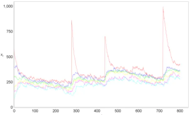
In Fig. 3, we can see the system ofm = 50nodes operating in nonstationary case with the control protocol (17). Each line indicates how the load xi
t evolves over time. For clarity, the
chart displays 3 maximum and 3 minimum values. These lines also show how the system evolves to reach load-balancing or consensus. We can see that even when the new burst task set is received during the system work, it does not affect the quality of load balancing. During the simulation we have set the coefficientα= 0.007, which is the most suitable value for the current topology and chosen parameters (see Fig. 2). In addition
Fig. 2. Rate of convergence based onα.
to the obtained results, it is planned to study the possibility of SPSA application for tracking the optimal value ofα.
Fig. 3. Perfomance of the system withm= 50nodesxi tfor the
nonstationary case.
8. CONCLUSION
In this paper the problem of load balancing in a multi-agent sys-tem underunknown but boundeddisturbances was examined. To solve the load balancing problem the new randomized lo-cal voting protocol with nonvanishing step-size was proposed. Conditions for achieving an approximate consensus (balance of the network load) were obtained. To illustrate the theoretical results we presented the simulations for the computing network.
REFERENCES
Amelin, K., Amelina, N., Granichin, O., Granichina, O., and Andrievsky, B. (2013). Randomized algorithm for uavs group flight optimization.11th IFAC International Workshop on Adaptation and Learning in Control and Signal Process-ing, 205–208.
Amelina, N. and Fradkov, A. (2012). Approximate consensus in the dynamic stochastic network with incomplete information and measurement delays. Automation and Remote Control, 73(11), 1765–1783.
Amelina, N., Fradkov, A., Jiang, Y., and Vergados, D. (2015). Approximate consensus in stochastic networks with applica-tion to load balancing. IEEE Transactions on Information Theory, 61(4), 1739–1752.
Boyd, S., Ghosh, A., Prabhakar, B., and Shah, D. (2006). Ran-domized gossip algorithms. IEEE Transactions on Informa-tion Theory, 52(6), 2508–2530.
Chebotarev, P.Y. and Agaev, R.P. (2009). Coordination in multi-agent systems and laplacian spectra of digraphs.Automation and Remote Control, 70(3), 469–483.
Granichin, O. and Amelina, N. (2015). Simultaneous pertur-bation stochastic approximation for tracking under unknown but bounded disturbances. IEEE Transactions on Automatic Control, 60(5).
Granichin, O., Skobelev, P., Lada, A., Mayorov, I., and Tsarev, A. (2012). Comparing adaptive and non-adaptive models of cargo transportation in multi-agent system for real time truck scheduling. Proceedings of the 4th International Joint Conference on Computational Intelligence, 282–285. Granichin, O., Volkovich, Z.V., and Toledano-Kitai, D. (2015).
Randomized Algorithms in Automatic Control and Data Min-ing. Springer.
Granichin, O. (1989). A stochastic recursive procedure with correlated noise in the observation, that employs trial per-turbations at the input. Vestnik Leningrad University: Math, 22(1), 27–31.
Granichin, O. (1992). Unknown function minimum point estimation under dependent noise. Problems of Information Transmission, 28(2), 16–20.
Granichin, O. (2015). Stochastic approximation search algo-rithms with randomization at the input. Automation and Remote Control, 76(5), 761–774.
Huang, M. and Manton, J. (2009). Coordination and consensus of networked agents with noisy measurements: stochastic al-gorithms and asymptotic behavior.SIAM Journal on Control and Optimization, 48(1), 134–161.
Kar, S. and Moura, J.M. (2009). Distributed consensus algo-rithms in sensor networks with imperfect communication: Link failures and channel noise. IEEE Transactions on Sig-nal Processing, 57(1), 355–369.
Lewis, F.L., Zhang, H., Hengster-Movric, K., and Das, A. (2014).Cooperative control of multi-agent systems: optimal and adaptive design approaches. Springer Publishing Com-pany, Incorporated.
Li, T. and Zhang, J. (2009). Mean square average-consensus under measurement noises and fixed topologies: Necessary and sufficient conditions.Automatica, 45(8), 1929–1936. Olfati-Saber, R., Fax, J., and Murray, R. (2007). Consensus and
cooperation in networked multi-agent systems. Proceedings of the IEEE, 95(1), 215–233.
Olfati-Saber, R. and Murray, R. (2004). Consensus problems in networks of agents with switching topology and time-delays. IEEE Transactions on Automatic Control, 49(9), 1520–1533. Polyak, B.T. and Tsybakov, A.B. (1990). Optimal order of accuracy of search algorithms in stochastic optimization. Problemy Peredachi Informatsii, 26(2), 45–53.
Rastrigin, L. (1963). The convergence of the random search method in the extremal control of a many-parameter system. Automation and Remote Control, 24(10), 1337–1342. Ren, W. and Beard, R. (2008).Distributed Consensus in
Multi-vehicle Cooperative Control. Communications and Control Engineering. Springer.
Ren, W., Beard, R., and Atkins, E. (2007). Information con-sensus in multivehicle cooperative control.Control Systems, IEEE, 27(2), 71–82.
Spall, J.C. (1992). Multivariate stochastic approximation using a simultaneous perturbation gradient approximation. IEEE Transactions on Automatic Control, 37(3), 332–341. Tsitsiklis, J., Bertsekas, D., and Athans, M. (1986). Distributed
asynchronous deterministic and stochastic gradient optimiza-tion algorithms. IEEE Transactions on Automatic Control, 31(9), 803–812.