Three-Dimensional Indoor RFID Localization System

(1)

DigitalCommons@University of Nebraska - Lincoln

Industrial and Management Systems

Engineering -- Dissertations and Student Research

Industrial and Management Systems Engineering

12-2012

Three-Dimensional Indoor RFID Localization System

Jiaqing Wu

University of Nebraska-Lincoln, [email protected]

Follow this and additional works at: https://digitalcommons.unl.edu/imsediss

Part of the Industrial Engineering Commons, and the Other Electrical and Computer Engineering Commons

Wu, Jiaqing, "Three-Dimensional Indoor RFID Localization System" (2012). Industrial and Management Systems Engineering -- Dissertations and Student Research. 36.

https://digitalcommons.unl.edu/imsediss/36

This Article is brought to you for free and open access by the Industrial and Management Systems Engineering at DigitalCommons@University of Nebraska - Lincoln. It has been accepted for inclusion in Industrial and Management Systems Engineering -- Dissertations and Student Research by an authorized administrator of

(2)

by Jiaqing Wu

A DISSERTATION

Presented to the Faculty of

The Graduate College at the University of Nebraska In Partial Fulfillment of Requirements For the Degree of Doctor of Philosophy

Major: Engineering

(Industrial, Management Systems, and Manufacturing Engineering)

Under the Supervision of Professor Robert E. Williams

Lincoln, Nebraska

(3)

Jiaqing Wu, Ph.D. University of Nebraska, 2012

Adviser: Robert E. Williams

Radio Frequency Identification (RFID) is an information exchange technology based on radio waves communication. It is also a possible solution to indoor localization. Due to multipath propagation and anisotropic interference in the indoor environment, theoretical propagation models are generally not sufficient for RFID-based localization. In fact, the radio frequency (RF) signal distribution may not even be monotonic and this makes range-based localization algorithms less accurate. On the other hand, range free localization algorithms, such as k Nearest-Neighbor (kNN), require reference tags to be spread throughout the whole three-dimensional (3D) space which is simply not practical. In this work, a hybrid real-time localization algorithm that combines reference tags with Received Signal Strength Indicator (RSSI) ranging is introduced to improve RFID-based 3D localization in high-complexity indoor environments. The experiments demonstrate that the proposed system is more accurate than traditional algorithms under real world constraints. The active RFID system includes 4 readers and 24 reference tags deployed in a fully furnished room. The localization algorithm is implemented in MATLAB and is synchronized with RF signal data collection in real-time. The results show that the novel

(4)

significant improvement over kNN and RSSI algorithms under the same circumstance. A battery-assisted passive RFID system was deployed side-by-side to the active system for comparison. Furthermore, the reader and tag performance was evaluated in both high-complexity laboratory environment and International Space Station (ISS) mock-up with high-reflection interior surface. In addition, theoretical models on minimum number of required reference tags and localization error prediction were introduced.

(5)

Acknowledgements

I wish to thank my advisor Dr. Robert E. Williams for his constant guidance, help, and support. His dedication to research has been a real inspiration.

I am sincerely thankful to Dr. Kamlakar P. Rajurkar, Dr. Michael W. Riley, and Dr. Lance C. Pérez for serving on my Ph.D. committee and providing valuable suggestions and comments to the original manuscript.

The dissertation experimentation would not have been possible without the

gracious use of the facilities of Dr. Lance C. Pérez, the MC2 laboratory in the department

of Electrical Engineering. I want to thank Lianlin Zhao, Marques L. King and all associates who were so friendly and helpful to my research there.

I would like to thank all faculty and staff members in the IMSE department and then the MME department since August 2011. Their kindness made my study at UNL much more comfortable.

I also would like to thank my beautiful wife, Bijia, for her love, caring, courage, and support during this research.

Finally, I dedicate this dissertation to my parents, Shuliang Wu and Zhenyun Cao, and to my sister, Jiawei Wu. They had a great influence on my career path and academic motivation and pursuits.

(6)

List of Figures

Figure 2-1: Typical frequency bands used for RFID ... 6

Figure 2-2: Communication models between RFID tags and readers ... 7

Figure 2-3: Active RFID tag structure ... 8

Figure 2-4: Two common RTLS schemes ... 20

Figure 2-5: RSSI with fingerprinting ... 22

Figure 2-6: Triangulation for AOA... 23

Figure 2-7: Cycle intersection for TOA ... 24

Figure 2-8: First step of multilateration for TDOA ... 25

Figure 2-9: Multilateration for APM ... 26

Figure 2-10: kNN ... 27

Figure 2-11: Proximity ... 28

Figure 3-1: Reader layout scheme ... 34

Figure 3-2: Tag layout scheme ... 34

Figure 3-3: Tag layout scheme (more)... 42

Figure 4-1: Layout scheme of reader test ... 49

Figure 4-2: Layout scheme of tag test... 52

Figure 4-3: Layout scheme of ranging test ... 54

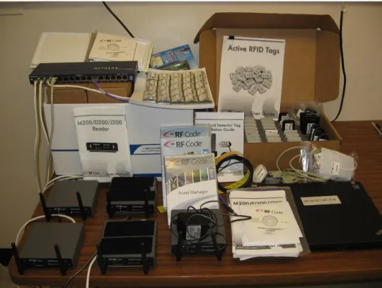
Figure 4-4: RF Code readers and tags... 55

(11)

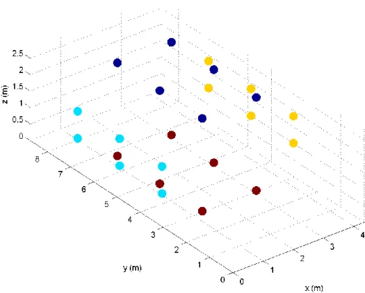
Figure 4-6: Reference tag layout in room environment ... 57

Figure 4-7: Network and software structure of the RF Code system ... 60

Figure 4-8: RSSI reading GUI ... 61

Figure 4-9: Localization GUI... 62

Figure 4-10: 2D algorithm ... 64

Figure 4-11: Intersection point and surrounding reference tags ... 66

Figure 4-12: Intelleflex readers and tags ... 70

Figure 4-13: International space station mock-up ... 71

Figure 4-14: Network and software structure of the Intelleflex system ... 72

Figure 4-15: Network and software structure of both systems ... 73

Figure 5-1: Main effects plot for reader test ... 78

Figure 5-2: Interference caused by human activities nearby ... 79

Figure 5-3: Main effects plot for tag test ... 81

Figure 5-4: Interaction plot for tag test ... 82

Figure 5-5: Main effects plot for ranging test ... 84

Figure 5-6: Linear regression of ranging test ... 85

Figure 5-7: Localization error histogram with fit ... 88

Figure 5-8: Localization error comparison ... 90

Figure 5-9: Main effects plot for mean ... 94

Figure 5-10: Main effects plot for standard deviation ... 96

Figure 5-11: Linear regression of ranging test (battery-assisted passive system) ... 97

(12)

(13)

List of Tables

Table 2-1: RTLS products list... 13

Table 2-2: Indoor RTLS comparison based on different frequency bands being used .... 18

Table 2-3: Summary of localization algorithms in RFID-RTLS ... 29

Table 3-1: Design of experiment #1 ... 43

Table 3-2: Design of experiment #2 ... 44

Table 4-1: Main factors of reader test ... 48

Table 4-2: Main factors of tag test ... 51

Table 4-3: Reference tags ID and positions ... 58

Table 4-4: Main factors of localization test ... 67

Table 4-5: Tag position definition ... 67

Table 4-6: Main factors of battery-assisted passive tag test ... 74

Table 4-7: Main factors of localization test (battery-assisted passive sytem) ... 75

Table 5-1: Localization error distribution for all orientations ... 87

Table 5-2: Localization error distribution for orientation same as reference tags only .... 88

Table 5-3: Localization error comparison... 104

Table C-1: Reader test data sheet... 169

Table C-2: Tag test data sheet ... 171

Table C-3: Ranging test data sheet ... 173

(14)

(15)

Nomenclature and Abbreviations

2D Two-dimensional

3D Three-dimensional

A-GPS Assisted-GPS

AOA Angle of Arrival

APM Adaptive Power Multilateration

COTS Commercial off-the-shelf

dBm Ratio of measured power decibels (dB) to one milliwatt (mW)

EM Electromagnetic

EPC Electronic Product Code

Gbps Giga-bits-per-second

Gen 2 EPCglobal UHF Class 1 Generation 2

GPS Global Positioning System

GUI Graphic User Interface

HF High Frequency, 13.56 MHz

IC Integrated Circuit

IR Infrared, 300 GHz to 405 THz

ISS International Space Station

JSON JavaScript Object Notation

(16)

LF Low Frequency, 120–150 kHz

LOS Line-of-Sight

LSQ Least Squares Quadratic

MW Microwave Frequency, 2.4–5.8 GHz

PI Prediction Interval

QoS Quality of Service

RF Radio Frequency, 3 kHz to 300 GHz

RFID Radio Frequency Identification

RSSI Received Signal Strength Indication (unit: dBm)

RTLS Real-Time Localization System

TDOA Time Difference of Arrival

TOA Time of Arrival

UHF Ultra High Frequency, 433MHz, 868-870 MHz, and 902-928 MHz

UPC Universal Product Code

UWB Ultra Wide Band

WiFi Wireless Fidelity

WLAN Wireless Local Area Network

WSN Wireless Sensor Network

(17)

Chapter 1

Introduction

1.1

Radio Frequency Identification (RFID)

Radio Frequency Identification (RFID) is a radio wave transmission process between an interrogator and a transponder, also known as a reader and a tag. The tag is identified by responding to the information stored in its internal memory or from the attached sensors. The reader is usually connected to a computer with a database for further processing of received information or sensor data. RFID technology is widely applied in transportation payments, asset management, supply chains, logistics, animal tracking, libraries, and securities [1].

Based on their working mechanism, RFID tags can be categorized as active tags, passive tags and semi-passive tags. The active tags are self-powered and broadcast signals at preset intervals. They usually provide a larger read range. The passive tags and passive tags are only activated by the querying signal from the reader. The semi-passive tags use internal battery power to enhance the broadcasting signal strength, while the passive tags are much cheaper and smaller. The operating frequency bands used for RFID tags vary from kHz, MHz to GHz, which leads to different radio wave coupling modes and performance.

(18)

1.2

Real-Time Localization System (RTLS)

An emerging application of RFID is indoor Real-Time Localization Systems (RTLS), where satellite-based navigation techniques are limited by in-building coverage, and wireless network devices are relatively expensive and larger than RFID tags and therefore not suitable for small items. Other non RF-based techniques, such as visual, ultrasonic, infrared and laser localization, are vulnerable to environmental impacts and are restricted to the Line-of-Sight (LOS) readability. Admittedly, the multi-path propagation is an issue for RFID localization.

Due to the variation of RF signals in a real indoor environment, the theoretical propagation model is not applicable for RFID localization. Numerous positioning algorithms have been developed. The multilateration approach utilizes different techniques for estimating distance between the unknown targets and the readers, such as, Received Signal Strength Indication (RSSI), Time of Arrival (TOA), and Angle of Arrival (AOA). The Bayesian inference approach statistically analyzes the dynamical data based on the Markov assumption. It is effective in tracking mobile objects upon calibration and training. In addition, both the k Nearest-Neighbor (kNN) approach by using weighted centroid of certain neighbors and the proximity approach by using intersection of several coverage areas, avoid the distance estimation step, but both heavily rely on the density of reference tags or reader distribution to improve positioning accuracy. Furthermore, most reported RFID-RTLS systems are designed for 2D space only, there is a clear need for a 3D system.

(19)

1.3

Purpose of Research

Due to multipath propagation and interference in the indoor environment, theoretical propagation models are generally not sufficient for RFID-based localization. In fact, the RF signal distribution may not even be monotonic and this makes range-based localization algorithms less accurate. On the other hand, range-free localization algorithms, such as kNN, require reference tags to be deployed throughout the whole 3D space which is simply not practical. Besides, the anisotropic environmental impacts in real 3D application are significant and not neglectable.

The first objective of this study is to model the theoretical minimum number of reference tags needed in a localization system. The modeling process is also helpful on identifying the major factor affecting the localization accuracy.

The second objective of this research, therefore, is to build an indoor RFID-based RTLS capable of positioning objects in 3D space in real-time. An active RFID system and a power-assisted passive RFID system were built side-by-side for easy comparison. The systems were deployed in a high-complexity laboratory room to reflect real environmental impacts.

The third objective of this dissertation is to investigate the RFID tag performance difference between the regular laboratory environment and the ISS mock-up. The high-reflection interior surface would be a big challenge for RF signal stability. The investigation result may be valuable for further system design.

(20)

1.4

Dissertation Organization

Chapter 2 consists of a literature review describing the background regarding RFID and RTLS technologies, their applications, and common system designs.

Chapter 3 presents a theoretical analysis about the minimum number of reference tags needed in a localization system.

Chapter 4 describes the proposed 3D localization system designs in the high-complexity environment and the localization algorithm being evaluated. The experiment designs of several fundamental tests are mentioned as well.

Chapter 5 contains the results and analysis of the fundamental tests and localization experiments. It also includes a tag performance comparison between active tags versus battery-assisted passive tags in both laboratory and mock-up environments.

Chapter 6 summarizes the conclusions and recommendations.

The appendices include the programming interface to the two types of readers, the Matlab codes used for controlling the whole system, and the data sheets for all experiments.

(21)

Chapter 2

Literature Review

2.1

Radio Frequency Identification (RFID)

Radio Frequency Identification (RFID) is a popular information exchange technology widely applied in electronic passport [2], animal tracking [3], supply chains [4], industrial automation [5], mining securities [6], hospital [7], asset management [8], and pharmaceuticals [9]. There are numerous RFID applications, and cannot be listed here completely. More examples may be found in the RFID Journal and RFID handbook [1, 10].

A simplest RFID system consists of two major components: a tag and a reader. The tag and the reader communicate via radio waves. The radio frequency (RF) bands commonly used in RFID include 120-150 kHz at Low Frequency (LF), 13.56 MHz at High Frequency (HF), 433MHz, 868-870 MHz, and 902-928 MHz at Ultra High Frequency (UHF), and 2.4-5.8 GHz at Microwave Frequency (MW) [10]. The RFID systems with operating frequency at LF and HF work based on inductive coupling. By contrast, the systems in the range of UHF and MW are coupled using electromagnetic (EM) fields, which brings a significantly higher read range than inductive systems.

(22)

These typical frequency bands used in RFID are summarized in Figure 2-1. The 433 MHz UHF and MW tags are usually used for active tags. In addition, the MW tags can be designed to be compatible with existing WiFi systems via the IEEE 802.11 protocols. For common passive RFID applications, the LF and HF tags can be used without license globally, while the UHF frequency bands are restricted by various regulations in different countries. These passive tags are most likely bonded with an Electronic Product Code (EPC), which is designed to enhance the traditional Universal Product Code (UPC) electronically. The international standardization of EPC is mostly led by EPCGlobal, an organization aiming to standardize and promote EPC technology worldwide. According to the latest standard [11], which is also adopted as part of ISO-18000, 868-870 MHz and 902-928 MHz readers and tags communicate using the EPCglobal UHF Class 1 Generation 2 (Gen 2) interface. The new protocol address some problems experienced from previous one used for LF and HF tags, namely Gen 1 tags.

Figure 2-1: Typical frequency bands used for RFID Low Frequency (LF) High Frequency (HF) Ultra High Frequency (UHF) Microwave Frequency (MW) 125-134 kHz 13.56 MHz 433MHz, 868-870 MHz and 902-928 MHz 2.4-5.8 GHz Near-field inductive coupling Far-field electromagnetic coupling

(23)

Normally, a reader initiates an inquiry or update process, as shown in Figure 2-2 part (a). Then, a tag receiving the command carries the order and replies the execution result to the reader. As shown in Figure 2-2 part (b), the self-powered active tag can be programmed to broadcast data periodically, regardless of whether any reader actually exists or not. The basic information reported by a RFID tag may include serial number, manufacturing date, vendor name, asset information, and other customized data [11]. Such static data is stored in the internal memory of the tag. For tags with rewritable memory, the data can be updated upon request. By integrating certain sensors to the tag, some additional information, such as motion status, air pressure, temperature, and humidity can be detected and reported by the tag as well.

Figure 2-2: Communication models between RFID tags and readers

Reader Tag

Inquiry/Update Response

Reader Broadcast Tag

(a) Inquiry/Update process

(24)

2.1.1

Figure 2-3: Active RFID tag structure

Based on different power source and working mechanism, RFID tags can be categorized into three major types: passive, semi-passive, and active tags. Both passive tag and semi-passive tag are activated by the querying RF signal from the reader. The passive tag is only powered by the energy transformed from the querying RF waves, which significantly decreases its read range, cost and size. On the other hand, the

semi-Antenna Coil Integrated Circuit (IC) Battery Sensor motion status, air pressure, temperature and humidity RF

(25)

passive tag uses internal battery power to drive the circuits and any existing sensors, and the signal transmission is still powered by the incoming RF waves. An active tag is self-powered and broadcasts signals at preset intervals. It usually provides a larger read range.

All types of tags are used in RFID-based RTLS. Systems using active tags are more commonly reported than passive tag systems due to the larger read range and continuously working ability. On the other hand, the passive tags and semi-passive tags have advantages on security and interference issues, owing to their silent characteristics.

2.1.1.1Passive Tags

A passive RFID tag has neither battery nor sensor. The RF waves propagated by the reader’s antennas are inducted to provide power for the passive tag. It appears to be dormant most of the time, and becomes active after an interrogation from a reader is received. The inquiry/response process limits the passive tag to communicate with only one reader at a time.

Typical operating frequency bands for passive tags are 120-150 kHz and 13.56 MHz. In this case, near-field communication, where the distance traveled in space of the RF signal is much less than its wavelength, acts as the major technology to drive the tag. A relatively larger coil, therefore, is required for the passive tag to generate enough power by inductive coupling. Since the RF signal strength decays along the distance rapidly, the read range of traditional passive tags is limited to 1 to 3 meters, varying by the operating frequency [12]. Due to the reflective characteristics of electromagnetic waves on metal and liquid surfaces, the readability of passive tags is severely affected

(26)

under such circumstances. The Gen 2 passive tags use 868-870 MHz and 902-928 MHz as operating frequency bands and are able to work in the dual mode of near-field and far-field communication, which improves the overall performance significantly. For instance, the read range can be extended to 10 meters [13].

Lack of a battery and a sensor definitely bring some limitations to passive RFID tags. But it also reduces the cost and size of RFID tags significantly.

2.1.1.2Semi-passive Tags

A semi-passive RFID tag is essentially a passive tag with additional battery and/or sensor. It is an enhanced edition of a passive tag, but not a silent edition of an active tag. The additional power supply is used to power the circuits and sensors only. In this way, all the power received via the RF waves can be used for RF communication with the reader. It marginally increases the read range since no more power in the received RF signal is shared to drive circuits the way passive tags do. As long as the inquiry signal can be received, the response can be sent back with full strength.

2.1.1.3Active Tags

With an additional battery as power supply, an active RFID tag has the ability to broadcast its identification information or sensor data actively and periodically. Therefore, active tags are able to communicate with multiple readers concurrently. Additionally, they have the larger read range between 50 to 100 meters as higher frequencies are used and broadcasting RF signal strength is enhanced with the extra battery [14].

(27)

Typical operating frequency bands for active tags are 433 MHz and 2.4 – 5.8 GHz, at which the RFID system works in the far-field region where the distance traveled in space of the RF signal is much greater than its wavelength. In such cases, using higher frequency (such as 2.4 GHz) leads to higher data transmitting bandwidth and rate. Therefore, new functionalities, such as tag-to-tag communication and integration to WiFi network, become possible.

The battery life of an active RFID tag is usually around 3 to 5 years. Thus, battery monitoring and maintenance are required. Moreover, the additional battery and related circuits increase both the cost and size of active tags significantly, comparing to passive tags.

2.1.2

Readers

A RFID reader is a device modulating and demodulating RF signals to communicate with supported RFID tags via one or several antennas. Most readers are compatible with either active tags or passive tags of certain operating frequency; only a few are able to work in dual mode. A database for managing all readers and tags, and some complicated control logics, such as noise threshold setting, antennas balance, and active history, may be deployed on the computer connected to the readers.

(28)

2.2

Real-Time Localization System (RTLS)

An emerging application of RFID is indoor Real-Time Localization System (RTLS), where the Global Positioning System (GPS) technique is limited by in-building coverage, Wireless Local Area Network (WLAN) devices are relatively expensive and larger than RFID tags and therefore not suitable for small items, and Ultra Wide Band (UWB) systems have a potential interference with some radar systems by sharing a wide range of bandwidth. Other non RF-based techniques, such as ultrasonic, infrared (IR) and laser localization, are vulnerable to environmental impacts and are restricted to the Line-of-Sight (LOS) readability. Admittedly, the multi-path propagation is an issue for RFID localization.

RTLS, especially indoor RTLS, has widespread applications in many areas. Most current systems provide room-level or sub-room level resolution. Low cost rack-level or item-level solution is desired. An uncompleted list of up-to-date RTLS products and their major applications is listed in Table 2-1. All information is collected from the product description available on their official websites.

(29)

Ta b le 2 -1 : RTLS p ro d u cts l ist S y ste m V e n d o r Te ch n o lo g y Ra n g in g Ac cu ra cy App li ca tio n s A ero S co u t RT L S A ero S co u t W iF i an d A cti v e RF ID T DO A , RS S I 5 m eter He alt h ca re , M an u fa ctu rin g , L o g isti cs ZO MOFI A lb is A cti v e RF ID 0 .5 2m Aw are n et Aw are p o in t Zi g Be e 1 -3 m eter He alt h ca re Ax ce ss RTL S Ax ce ss A cti v e RF ID L o g isti cs, S ec u rit y Ce n T ra k R TL S Ce n T ra k In fra re d a n d A cti v e RF ID Ra ck -le v el He alt h ca re W irele ss L o ca ti o n Cisc o W iF i, A cti v e an d P ass iv e RF ID A sse t M an ag e m en t Ek ak au R T L S Ek ak au W iF i RS S I S u b -r o o m He alt h ca re , Re tail, L o g ictics , M a n u fa ctu rin g L OS T Esse n siu m Zi g Be e T O A S u b -m eter L o g isti cs A rg u s G u ard RF ID A cti v e RF ID 3 -5 m eter In d u strial, He alt h ca re S en so rS M A RT Id en tec A cti v e RF ID an d W S N M arin e, Oil, M in in g , De fe n se In S it es L o ca to r In telli g en t In S it es V ario u s tec h n iq u es Ro o m -lev el He alt h ca re BizT al k RF ID M icro so ft UW B an d RF ID M an u fa ctu rin g RTL S EN G IN E Mo to ro la W iF i, A ctiv e and P as siv e RF ID A ss et Ma n ag e m en t O m n it ro l RT L S O m n it ro l W iF i, UW B, a n d RF ID M an u fa ctu rin g , Re tail, L o g isti cs P an G o L o ca to r P an G o /Ci sc o W iF i an d A cti v e RF ID RS S I A sse t M an ag e m en t, He alt h ca re P erv T ra ck R TL S P erv Co m A cti v e RF ID an d W S N M an u fa ctu rin g , M in in g I n d u stry P INC RT L S P INC P ass iv e RF ID +/ - 1 sp o t Ya rd M an ag e m en t P in P o in t RT L S P in P o in t W iF i an d Zi g Be e Ed u ca ti o n , He alt h ca re , Ho sp it ali ty iL o ca te P re cy se W S N M an u fa ctu rin g , De fe n se , Re tail, He alt h ca re Ra d ian se RT L S Ra d ian se A cti v e RF ID He alt h ca re A sse t M an ag er RF Co d e A cti v e RF ID S u b -r o o m A sse t M an ag e m en t Ro o m L o ca to r RF Co d e In fra re d Ra ck -le v el A sse t M an ag e m en t RFin d RT L S RFin d A cti v e RF ID A u to m o tiv e, L o g istic s, Ma n u fa ct u rin g , Pu b lic T ra n sit S m artCh ain S av i A cti v e RF ID A ero sp ac e, De fe n se , L o g isti cs, N atu ra l Re so u rc es Hig h De fin it io n S o n ito r/IB M Ultras o u n d S u b -r o o m He alt h ca re , Ho m ec are P lu s, P lu sO N T im e Do m ain UW B Re tail, M an u fa ctu rin g , He alt h ca re , De fe n se Ub ise n se RT L S Ub ise n se UW B A O A , T DO A 1 5 cm M an u fa ctu rin g , De fe n se , T ra n sp o tatio n El p as V iso n ic In fra re d , A cti v e an d P ass iv e RF ID He alt h ca re W a v etren d S y ste m W a v etren d A cti v e RF ID Co n stru cti o n , Oil an d G as, De fe n se , S ec u rit y , M in in g V isib il it y S y ste m W estico W iF i M eters L o g isti cs, Re tail, M an u fa ctu rin g , He alt h ca re Mo b iW ER X W ire le ss W ERX Blu eto o th H o sp itality , Re ta il, A ttra ctio n s, Mo b ile -g a m in g W h ere Ne t Zeb ra W iF i an d UW B T DO A A sse t T ra ck in g , S u p p ly Ch ain M an ag e m en t

(30)

2.2.1

Global Positioning System (GPS) and A-GPS (Assisted GPS)

The Global Positioning System (GPS) is a well-known satellites-based outdoor localization system operated by the U.S. Other similar systems in use include: GLONASS by Russia, Beidou by China, and Galileo by Europe. Assisted GPS (A-GPS) is a GPS application which uses cellular network resources to improve the startup and locating performance of a receiver. By measuring the time difference of arrivals from four or more satellites at the same time, the GPS receiver is able to calculate its three-dimensional (3D) position based on the multilateration approach. For civil applications, the positioning resolution is about 10 meters for outdoor usage [15]. However, neither GPS nor A-GPS is suitable for indoor applications due to weak signals. Furthermore, high energy consuming and expensive receivers limit the GPS or A-GPS to be used for a large scale deployment.

2.2.2

Wireless Local Area Network (WLAN) and Wireless Sensor

Network (WSN)

The Wireless Local Area Network (WLAN) technique is used for indoor localization due to several advantages against GPS/A-GPS. First, the Wireless Fidelity (WiFi) devices are relatively inexpensive and have low power consumption. Second, WiFi network become an increasingly common infrastructure in many buildings, which help to reduce the deployment cycle and overall cost of a WiFi-based indoor localization system. Nevertheless, the size, cost and power consumption of traditional WLAN devices are still not comparative to RFID tags due to different purpose of use. A technique called

(31)

Wireless Sensor Network (WSN) was developed to address such issues. The idea of WSN is to limit the computational power and signal bandwidth of a WSN node to a low level so that the overall performance is just enough for environmental monitoring applications. Then, a new problem emerges. WSN nodes may be interfered by WLAN devices which usually have stronger signals. ZigBee and WiFi are two most important protocols used in WSN. One of WSN’s major advantages is inter-communication capability among nodes. The positioning accuracy of the WiFi-based localization systems varies from sub-meter to several meters for different algorithms and deployment densities [16]. According to latest research results, the accuracy could achieve 0.04 meters for 2D and around 0.1 meters for 3D applications [17, 18].

2.2.3

Radio Frequency Identification (RFID)

The biggest advantages of passive or semi-passive RFID tags are the extremely low price and ultra-small size. However, the RTLS applications based on Gen 1 passive/semi-passive RFID tags are limited by the low read range. Dense deployment is required to provide enough coverage. The typical resolution of such a RTLS is at the sub-meter level and highly depends on the density of tag deployment. A system may benefit from the larger read range of Gen 2 passive tags. For all kinds of passive tags, the tag orientation affects the signal reading significantly [19]. A common solution is to fix all tags, both reference tags and target tags, on the same plane (ceiling, floor, or wall) with the same orientation [20, 21]. This certainly causes some limitations in real applications.

(32)

Active RFID is similar to WSN but differs in that it has lower operation frequency (except for WiFi-based RFID, which will be discussed later) and lacks tag-to-tag communication feature. Due to similar mechanism, most deployment schemes and positioning algorithms work in almost the same way for both active RFID and WSN localization systems. Consequently, they share the localization resolution from sub-meter to sub-room level as well. The 433 MHz RFID system has a potential to be interfered in real applications because this frequency band is open for amateur radio [10]. The term, WiFi-based RFID particularly refers to a RFID system operates at the frequency of 2.4 GHz and is embedded into or able to communicate with any existing WiFi systems. In this way, the RFID system can be easily deployed and managed. Though, interference and traffic control between RFID signals and regular WiFi signals requires additional Quality of Service (QoS) configuration on the network server [22].

2.2.4

Ultra Wide Band (UWB)

As a totally different approach, Ultra Wide Band (UWB) is a radio technique which has high volume data rate (up to 1 Gbps) as the result of using ultra-short pulses (up to 1-2 giga-pulses per second) over a wide range of frequency spectrum (from 3.1 to 10.6 GHz) [23]. In general, the positioning resolution of a UWB-based localization system can achieve decimeter level, via LOS measurement and multilateration approximation [12]. Some particular algorithms may result in even more accurate resolution, less than 0.04 meters [23]. The pulse radio transmission style ensures UWB have no interference with other narrow-banded wave radio transmissions in the same

(33)

frequency bands. However, it may be interfered in some environments where air traffic control radio beacon system, airport or maritime surveillance radar, and GPS receivers, are in use [24]. Another concern is that various regulations on this wide spectrum are permitted in different countries [25], because the pulse-based radio technique is originally reserved for military usage, such as radar and satellite systems. This leads to high R&D cost and, therefore, high price for UWB chips.

2.2.5

Non RF-based

Other than the above mentioned radio-based solutions, those non RF-based techniques, such as ultrasonic, infrared (IR) and laser localization, have long been applied in positioning systems and are mature [14]. However, restricted to the Line-of-Sight (LOS) readability, these techniques are vulnerable to environmental impacts, for instance, obstacles and irregular room shapes. On the other hand, such LOS characteristic ensures item-level accuracy, given the tag is detected. Nevertheless, the overall locating resolution is highly determined by the density of reader/antenna deployment, which leads to significantly increased cost of the whole system.

(34)

2.2.6

Summary

Upon the above discussion, several interesting characteristics of the indoor RTLS with various techniques are summarized and compared in Table 2-2. The unit accuracy column defines the accuracy level being achieved by a single unit but not the whole system, since some systems’ resolution highly relies on the density of tag/reader deployment. It should be noted that the system cost column is comparing the estimated building cost of a system based on comparative overall performance.

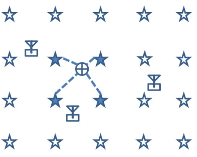
Table 2-2: Indoor RTLS comparison based on different frequency bands being used

Category Frequency Band Unit

Accuracy

LOS Multi-path

Read Range

EM IR/Laser High Wide High Yes No Medium

RF UWB High Wide High No No Medium

Narrow Band

MW* Medium Medium Med/High No Yes High

UHF Medium Medium Medium No Yes Med/High

HF Low Narrow Medium No Yes Medium

LF Low Narrow Low No Yes Low

Ultrasound Low Narrow High Yes Yes High

*Note: Both WLAN/WSN and WiFi-based RFID are included in the MW band.

As a whole, the UWB, WSN, and Gen 2 RFID techniques seem to stand out from the others. Due to the low price of tags, Gen 2 RFID technique is very suitable for large scale applications. Though, its localization accuracy is lower than the other two.

(35)

2.3

RFID-RTLS

Despite the difference caused by various types of RFID tags, the fundamental system structure, or scheme of RFID-RTLS varies. Also, different positioning logics, namely algorithms, have been reported.

2.3.1

Schemes

RFID-based localization can be classified as tag localization and fixed-reader/antenna localization, in accordance with different roles of tags and readers/antennas [26], as illustrated in Figure 2-4. In the fixed-tag scheme, the tags are deployed on the ceiling or floor with some rules while the readers/antennas are usually attached to mobile objects. This is cost effective when the objects to be tracked are relatively large, few in numbers, and usually move in a 2D plane or on a certain route. The major application is an auto guided vehicle or robot [27, 28]. In the fixed-reader/antenna scheme, the readers/antennas and tags are placed in an opposite way to the fixed-tag scheme. The readers/antennas are installed at fixed positions while the tags are attached to the items to be tracked. It is useful for most applications where a lot of items need to be tracked and located at the same time because the tags are much cheaper and smaller than the readers/antennas. The following work will be based on this scheme.

(36)

(a) Fixed-tag scheme (b) Fixed-reader scheme

Figure 2-4: Two common RTLS schemes

2.3.2

Algorithms

In a real indoor environment, fading, absorbing, reflection, and interference are major issues affecting the RF waves’ strength, direction, and distribution. This make the variation of the RF signal propagation not easily modeled. Since the theoretical model is not applicable, numerous positioning algorithms have been developed. Several major types are summarized and introduced as follows, while many varieties exist. The two largest groups are determined by whether the algorithm ranges the RF signal to an estimated distance or not.

The range-based localization algorithms require two steps of work. First, the elementary range results are obtained in several ways: Received Signal Strength

Reader Tag Tag Tag Tag Tag Reader Reader Reader Reader

(37)

Indication (RSSI), Angle of Arrival (AOA), Time of Arrival (TOA), Time Difference of Arrival (TDOA), or Adaptive Power Multilateration (APM). Then, various approaches on geographical calculations, such as triangulation, trilateration, and multilateration, are applied to estimate the final position.

Both the k Nearest-Neighbor (kNN) approach by using centroid of certain neighbors and the proximity approach by using intersection of several coverage areas avoid the distance estimation step in range-based localization approaches. However, they heavily rely on the density of reference tags or reader/antenna distribution to improve positioning accuracy.

2.3.3

Range-based Localization

2.3.3.1Received Signal Strength Indicator (RSSI)

Received Signal Strength Indicator (RSSI) is considered the simplest approach for ranging since almost no additional cost is needed to collect the RSSI data which is provided by most systems [29]. It is a measurement of received radio signal power in terms of the ratio of measured power decibels (dB) to one milliwatt (mW). However, it is also a less accurate way due to complicated environmental impacts to the RF signals propagation [30]. No theoretical or empirical model can be applied as a universal solution. Therefore, the RSSI map, which is used to translate the signal strength into distance estimation, should be calibrated for every single antenna to achieve better results. The initial solution is to measure the RSSI values at all possible points with predefined density and renew the mapping periodically. It is not practical to maintain such a system.

(38)

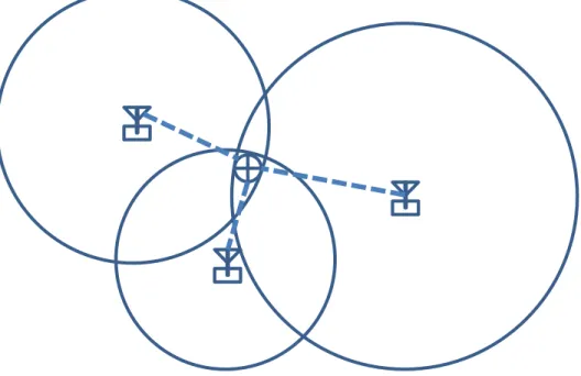
Later, a technique called fingerprinting, or profiling is used, which places reference tags at particular positions to serve as anchors. The signal strength collected from these reference tags with known coordinates help to build a dynamic RSSI map reflecting real environmental impacts. For each antenna, this map is used to translate the RSSI value from a tag with unknown coordinates into an estimated distance from this tag to the antenna. Classical lateration can be applied to collective data from several antennas to approximate the position of this unknown tag in space. The idea of RSSI with fingerprinting is demonstrated in Figure 2-5. The improvement on resolution relies on the density of these anchor nodes.

(39)

2.3.3.2Angle of Arrival (AOA)

The basic idea of Angle of Arrival (AOA) is simple. Consider a triangle for example. Given the coordinates of any two points are known, the third one can be located if and only if the angles from these two known points to the unknown point are provided. This method is known as triangulation, as illustrated in Figure 2-6. The concept can be extended to 3D space easily. This approach requires customized RF signal modulating/demodulating units which are add-ons to the overall cost. Therefore, precise calibration is needed before use. The LOS requirement is another limitation for applications. The measured angle accuracy is less than 1.7° in a small experimental space, and decreases for larger angles and longer distance between the tag and the antennas [31]. The overall resolution is approximately sub-meter level for a regular room size space, and depends on the density of reader/antenna deployment.

Figure 2-6: Triangulation for AOA

Two angles Known distance

(40)

2.3.3.3Time of Arrival (TOA)

The Time of Arrival (TOA) method is based on a theoretical propagation model of an RF signal. The distance between two points can be determined if the travel time of the signal between them is measurable. Then, the location of an unknown tag can be determined using such measurements from various antennas. Cycle intersection, as shown in Figure 2-7, and nonlinear least-squares approaches are commonly used to get optimal results with minimum errors. However, the velocity of the EM wave is so high that the typical travel time within a room is on the scale of nanoseconds. Hence, the TOA method requires all readers and tags to be strictly precisely synchronized, and all signals to be time-stamped [29]. The theoretical accuracy can be very high. But with affordable commercial synchronizing unit, the system resolution is usually about 1 to 2 meters [32]. Moreover, LOS is required to reduce interference caused by multi-path effects.

(41)

2.3.3.4Time Difference of Arrival (TDOA)

Similar to TOA, the Time Difference of Arrival (TDOA) approach also relies on precisely synchronized readers and tags. But it uses a different methodology to determine the location of the unknown point [33]. For each pair of antennas, given the time difference of the RF signals from them to the tag to be tracked is known, all the possible locations of this tag must fall into one half of a hyperbola in 2D space, as shown in Figure 2-8, or a hyperboloid in 3D space. Then, the tag’s location is determined as the intersection of the hyperbolas or hyperboloids generated by all pairs of antennas. The TDOA method has same limitations and drawbacks as TOA.

(42)

2.3.3.5Adaptive Power Multilateration (APM)

Another approach is called Adaptive Power Multilateration (APM), which measures the estimated distance from the reader to the tag by reducing or increasing the reader transmission power until the tag disappears or appears, as shown in Figure 2-9. The corresponding power level is then translated into distance based on a pre-calibrated chart. At last, the tag’s position is determined using the multilateration method on distances estimated from all readers. The accuracy of APM heavily relays on two things. One is the edge tolerance of the power circle. A perfect clear cut at the edge may not exist. The other one is the environmental impacts. The pre-calibrated chart may not be valid under complex circumstance. Some attempts were reported to improve this method by using reader rotating and some statistical analysis [34, 35].

(43)

2.3.4

Range-free Localization

2.3.4.1k Nearest-Neighbor (kNN)

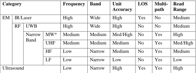
The fingerprinting technique applied in the improved RSSI approach is also used in the k Nearest-Neighbor (kNN) method but without ranging. Similarly, the reference anchors are deployed in cells. The Eucledian distances between the RSSI values from the unknown tag and all anchors are calculated. Subsequently, the k anchors with lowest distances to this tag are selected as its k nearest neighbors. The coordinates of this tag can be estimated using the centroid of these anchors, as illustrated in Figure 2-10. An enhanced method call weighted kNN further applies the Eucledian distances from the unknown tag to its k nearest neighbors as weights to improve the approximation [7]. Overall, the kNN approach is suitable for complex non-isotropic and varying environments.

(44)

2.3.4.2Proximity

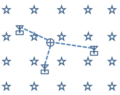
In the proximity approach [14], each antenna has a predefined coverage area, which may be an approximation or calibrated result. If the unknown tag is detected by more than one antenna, the location of this tag can be estimated by the intersection of the coverage areas of these antennas, as shown in Figure 2-11. The density of antenna deployment heavily affects the system resolution. Furthermore, the coverage area may be difficult to be clearly defined since the RF signals fade away gradually at the edge and the theoretical propagation model may not be an appropriate simulation for real indoor environments.

(45)

2.3.5

Summary

Pros and cons of different types of localization algorithms most commonly used in RFID-RTLS are summarized in Table 2-3. Reported localization errors for several systems using these algorithms are also listed.

Table 2-3: Summary of localization algorithms in RFID-RTLS

Algorithms Pros Cons Accuracy

Range-based

RSSI Low cost; supported by most systems; enhanced with profiling

Low accuracy level; relies on dense deployment of reference tags

0.5 m [36], simulated; 0.72 m [37], measured AOA High accuracy level High cost for customized

hardware; LOS measurement required; pre-calibration need

N/A

TOA High accuracy level High cost for synchronized devices; LOS measurement required

N/A

TDOA High accuracy level High cost for synchronized devices; LOS measurement required

0.2 m [38], measured APM Low cost; no reference

tags needed

Low accuracy level; relies on pre-calibrated power versus distance chart; not suitable in complex environments 0.32 m [35], simulated; 0.6 m [34], measured Range-free

kNN Low cost; suitable for complex non-isotropic and varying environments

Low accuracy level; relies on dense deployment of reference tags

0.6 m [7], measured Proximity Low cost; easily deployed Low accuracy level; relies on

dense deployment of readers or antennas, coverage areas may not be clearly defined in complex environments

(46)

Overall, the RSSI and kNN approaches are mostly cost effective and reliable for indoor environments. Actually, these two methods are very similar in that they share the fundamental step of fingerprinting the reference tags. They are only different in the final stage for estimating the position of the unknown tag.

(47)

Chapter 3

Theoretical Modeling

3.1

Introduction

It is of interest whether there is any statistically significant minimum number of reference tags needed for an indoor, real time localization system based on Gen 2 RFID with battery-assisted passive tags or other active tags. This problem may be solved in two steps.

First, find out a theoretical solution (at least approximation) based on a series of assumptions and experimental data from various sources.

Second, design an experiment which is able to determine the relationship between accuracy level and number of reference tags, and compare the result to the value estimated in first step.

Furthermore, the trend of localization error as the system dimension increases from 1D to 2D and then to 3D is investigated. It may be useful on predicting the 3D localization error based on previous 2D or 1D system performance.

(48)

3.2

Assumptions

The following are the assumptions used in this modeling section.

 Room size. To simplify the question, the test bed is assumed to be located in a

room with the dimension of 3x3x3 meters. In this way, all readers and tags can be deployed symmetrically and evenly in the 3D space. Such deployment policy in 2D is reported to be an optimum solution in terms of maximizing accuracy [39]. Furthermore, 3*√5=6.7 meter (the maximum distance within a 3x3x3 cube) is a safe distance to cover the read range of common Gen 2 RFID passive tags [40]. Larger room size may require either more readers or higher class tags to ensure the RSSI in a stable range. Either option leads to increased overall system cost.

 Environment. In reality, a complex environment is very difficult to be modeled.

So, the room is assumed to be absent of large obstructions. All environmental effects, such as radio wave reflection, absorption, and possible interference, are assumed to be isotropic and consistent.

 Reader. The amount of readers (and/or extended antennas, which will also be

treated as reader for the sake of conciseness) and their deployment will affect the localization algorithm and accuracy. Nevertheless, such variation/optimization is out of the scope of this question. Let’s assume that four readers are placed at the four opposite corners of the room and none of them are located on the same edge

(49)

of the cube, as illustrated in Figure 3-1. This is one of the symmetric layouts with minimum amount of readers required in a 3D space RTLS system.

 Tag. All reference tags are placed evenly and symmetrically on the six faces of

the cube. None of them is placed in the inner space of the cube, as this is not practical in any real application. So, the total amount of all reference tags with such criteria cannot be any possible integer. Only certain numbers of tags are possible. Therefore, the minimum amount is 6 for one on each face center. Several possible layouts are illustrated in Figure 3-2. Scheme (a) has one reference tag on each corner point. Scheme (b) has one reference tag on each edge center. Scheme (c) has one reference tag on each corner point, edge center, and face center. More tag layout schemes will be discussed later.

 Algorithm. To simplify the solution, the basic RSSI ranging approach is applied

to each reader. The RSSI map (based on all reference tags) for each reader is constructed and assumed to be isotropic in 3D space. The distances from the target tag to four readers are then estimated. The Trilateration method is used to determine the final position of the target tag.

 Measurement. The accuracy is defined as the distance from the real position and

the estimated position of a target tag. Theoretically, the accuracy is not the same everywhere since there is no reference tag in the middle of the room. So, it is best to place the target tag at any random position within the room to calculate the accuracy. However, this may involve complex modeling and simulation. In this

(50)

solution, therefore, the accuracy is averaged over the whole space with a few measurements.

Figure 3-1: Reader layout scheme

Figure 3-2: Tag layout scheme

(51)

3.3

Ranging

The theoretical propagation model used most extensively for RSSI ranging is called log-normal propagation model [12], which is valid with previous environmental assumptions. The model is given in Equation (3-1).

[ ] ( ) (3-1)

where PL(d0) is the path loss value for a reference distance d0 (commonly 1.0 meter), η is

the path loss exponent, and Xσ is a Gaussian random variable with zero mean and

variance, σ2, that models the random variation of the RSSI value.

According to previous research [41], the RSSI values are approximately linear within a range of 4 meters in the anechoic chamber and to a range of 10 meters in the clear hallway. Therefore, the propagation model in this question may be simplified into Equation (3-2).

[ ] ̂ ( ) ̂ (3-2)

where ̂ is the slope coefficient for distance, which is a value estimated from the linear

regression of measured RSSI for a given distance. It is a Gaussian random variable with

mean β and variance σβ2

(∑ ̂ ) (∑⁄ ( ̅) ) that models the random variation due to regression estimation. Obviously, more reference tags (larger n) lead to

smaller σβ2 and hence more precise estimation of β. It should be noted that, by definition,

(52)

is same as Xσ. Similarly, ̂ ( ) is the intercept coefficient with variance

( ∑ ).

In order to predict distance with given RSSI, the Equation (3-2) is transformed into Equation (3-3).

̂ ( ) ̂ [ ]

̂ (3-3)

where ̂ [ ] contains possible measurement error. Then, we have Equation (3-4).

( ̂ ( ) ̂ [ ]

̂ ) (3-4)

This can be further calculated via the following equations, referred from [42, 43].

( ) ( ) ( ) ( ) (3-5) ( ) [ ( )] ( ) [ ( )] ( ) ( ) ( ) (3-6) ( ) [ ( ) ( )] { ( ) [ ( )] ( ) [ ( )] ( ) ( ) ( )} (3-7)

The close form solution of may be too complicated to be easily interpreted. So,

pilot experiment results should be used for further evaluation. The values may vary for different systems and environments, but the derivation steps are the same. For example, based on the experiment results on active RFID tags in 2D space, the estimated

regression function (with 9 reference tags) is d = -9.560 - 0.234PRX. The varies from

0.126 to 0.430 (average 0.278) within the range of 4 meters. The corresponding 95% prediction interval (PI) for ranging varies from 1.858 to 2.690 meters (average 2.274).

(53)

A close investigation into the relationship between and n reveals that

( ) ( ) ( ) ( ) ( ) ( ) (3-8)

where Var(regression) is the variance generated from linear regression approximation

process, Var(nature) in the variance inherited from RSSI variation and measurement

error, Cov(r,n) is the covariance between them, and α(n), β(n), and γ(n) are corresponding

coefficients for the three terms, respectively. The three coefficients are functions of n.

A proposed hypothesis of as a function of n is that will decrease to a certain

level as n increases. After that, Var(nature) becomes dominant, and will keep nearly

constant. We may design a series of experiments with various amounts of reference tags to see whether we are able to fit a model to predict such trend or not. If it is found, then the maximum possible RSSI ranging error can be estimated for any given amount of reference tags.

(54)

3.4

Localization

After the approximated distances from the target tag to four readers are obtained, the relationship among them may be present in Equation (3-9).

{ ( ) ( ) ( ) ( ) ( ) ( ) ( ) ( ) ( ) ( ) ( ) ( ) (3-9)

where ( ) is the target tag coordinate to be estimated, ( ) is the position of

four readers, and ri are the predicted distance from the target tag to the four readers. This

group of nonlinear functions can be solved via traditional nonlinear least squares approach, iterative arithmetic method, or some other algorithms [44]. The fundamental

idea is to find the best solution of ( ) which minimizes the sum of squared

differences between the ri’s and their corresponding modeled values.

The final localization error, e, between the approximated position ( ̂ ̂ ̂) and the

real position ( ) of the target tag is defined in Equation (3-10).

( ̂) ( ̂) ( ̂) (3-10) According to the performance analysis presented in [44], the variance of the position estimation error is proportional to the square of ranging error, and can be modeled in Equation (3-11).

(55)

where is the random error inherited from the RSSI ranging process, , , and are geometric indices expressing the non-isotropic effect of the system, which can be calculated with the following functions of Equation (3-12).

(3-12)

By assuming isotropic everywhere in previous statement, the variances in three

axes are identical, and are equal to the ranging variance . Therefore, the geometric

indices , , and are all equal to √2. By further assuming no covariance among the

variances in three axes, the overall variance of position estimation error can be determined by Equation (3-13).

(3-13)

Similarly, the expected value of the localization error, namely bias, is also proved to be proportional to the square of ranging error, and can be modeled by Equation (3-14).

(3-14)

where , , and are geometric factors expressing the nonlinearity effect of the

system, which may be defined as the coefficients ratio of the second and first order terms of the nonlinear distribution equation. By assuming linearity everywhere in previous statement, the second order terms are negligible for all three axes. Therefore, the

geometric factors , , and and corresponding expected values of position

estimation error for all three axes are equal to zero. This means the overall estimation is unbiased, as shown in Equation (3-15).

(56)

( ) √ (3-15) The above result is based on a series of assumption which may not be adequate in a real situation, especially the non-isotropic characteristics of RSSI reading. It is known to be sensitive to the orientation of the tag with respect to the reader. It’s impossible to have all reference tags facing each reader with same orientation at the same time. Multiplicity of reference tags is a possible solution which will not be discussed here. Moreover, the ranging error must be different at various locations in the room since there is no reference tag in the middle of the room and the environmental factors will affect the reading close to the wall, floor, ceiling, or any area using certain materials such as metal. All of these will lead to a higher overall position estimation error than what has been derived here.

Since the 95% prediction interval (PI) is proportional to standard error, the projected 95% PI for 3D localization should be approximately √6 times of the 95% PI for

ranging only, based on Equation (3-13). Now, using the pilot result at n=9, the estimated

95% PI for 3D localization is about (2.274)*√6 = 5.57 meters. This means, with the linear regression function estimated from 9 reference tags and the position approximation via trilateration, we are 95% confident that the true position is within a 5.57 meters interval, which is the diameter of a globe centered at the approximated position of the target tag. In other words, the maximum possible error of the position estimation is 2.79 meters away from the true value. Moreover, it is possible to estimate this 95% PI with any amount of reference tags via the Equation (3-8) and Equation (3-13).

(57)

Please note that this is maximum possible error. It is different from the usually

defined average error. Theoretically, the average localization error, e, can be calculated

based on the definition in Equation (3-10) and its expected value √ ⁄ by assuming a

normal distribution, as shown in Equation (3-16).

̂ √ ⁄ √ ⁄ (√ ) √ ⁄ (3-16)

The estimated error for 3D localization, ̂, is then approximately 2 times of the

ranging standard deviation, . Since the definition of 95% PI is [μ-1.96σ, μ+1.96σ], or

approximately [μ-2σ, μ+2σ], Equation (3-16) can be further expressed in terms of 95% PI

for ranging only, as shown in Equation (3-17).

̂ (3-17)

Using pilot result at n=9, the estimated localization error for 3D is about

(2.274)*0.5=1.137 meters, which is expected to be close to the measured one, e. Though,

it is higher than the accuracy assumption of 0.5 meters, which means more reference tags may be desired to increase the accuracy level.

(58)

3.5

Experiments

The following proposed experiments involve two parts. The first one is to model

the regression function of RSSI ranging variance, , with amount of reference tags n.

The second one is to model the localization error, e, (which is approximately the double

of ranging standard deviation) with respect to amount of reference tags, n.

For both experiments, the factor being varied is the amount of reference tags.

Since n=9 was insufficient, we start from n=12. Five levels are enough to detect possible

high-order polynomial, logarithm, or Hoerl model trend using regression analysis [45].

These five levels (n=12, 18, 26, 42, and 48) will be implemented as illustrated in Figure

3-2 and Figure 3-3.

Figure 3-3: Tag layout scheme (more)

For experiment #1, the ultimate response variable is , the variance of distance

prediction using the corresponding linear regression estimation. The ultimate predictor

variable is n, the amount of reference tags. Nevertheless, is not directly measurable. It

(59)

should be estimated from the regression process, which is conducted by reader, a block

factor B. For each reader of a given scheme (with certain level of n), the RSSI value and

distance from every reference tag to the corresponding reader are measured to fit a

regression model (assumed to be linear). The for the four blocks are then averaged for

this level of n. By repeating this process for all schemes, we are able to fit the ultimate

regression model between and n for the purpose of predicting using arbitrary n.

The design structure of experiment #1 is summarized in Table 3-1.

Table 3-1: Design of experiment #1

Objective To fit the best model of ( )

Distance = f(RSSI) ↘ n=12 n=18 n=26 n=42 n=48 B=1 B=2 B=3 B=4 Average

For experiment #2, the ultimate response variable is the localization error, e. The

regression function of ( ) is easy to model. Though, it is of more interest whether

the relationship described in the Equation (3-13) is valid or not. The design structure of experiment #2 is summarized in Table 3-2. Please note that the total number of replicates (by putting target tags at different locations) is designed to be able to catch any sample

(60)

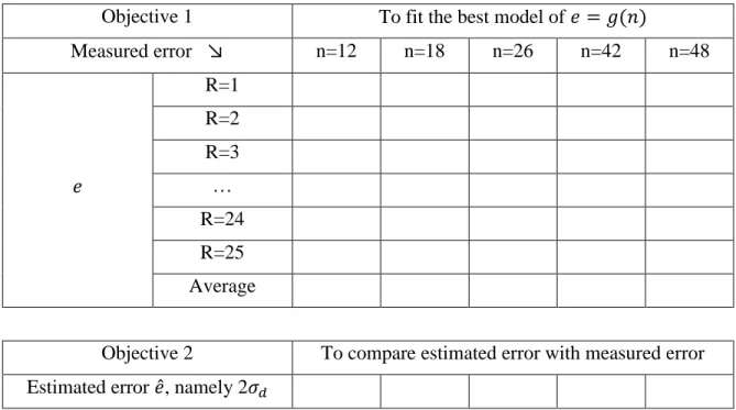
Table 3-2: Design of experiment #2

Objective 1 To fit the best model of ( )

Measured error ↘ n=12 n=18 n=26 n=42 n=48 R=1 R=2 R=3 … R=24 R=25 Average

Objective 2 To compare estimated error with measured error

(61)

3.6

Summary

Both theoretical analysis and experimental design are presented to demonstrate the idea of evaluating the statistically confident accuracy as a function of the amount of reference tags for an indoor RTLS with numerous assumptions. Therefore, the statistically significant minimum number of reference tags needed may be obtained in a reverse way. The theoretical model also indicates that a lower-bound of the accuracy level for any given system may exist, due to the natural variation of RFID signal strength. Improved system design and ingenious localization algorithm may help make this lower-bound even smaller.

The experimental results could differ a lot from the theoretical function due to violation of those assumptions or restrictions of the test environment. Revised prediction model is expected to include more variables, rather than the number of reference tags only. Despite these, there are several important conclusions which may benefit further research.

The ranging accuracy is affected by both the regression analysis and the RSSI variation, as shown in Equation (3-8). At some point, the increase