East Tennessee State University
Digital Commons @ East
Tennessee State University
Electronic Theses and Dissertations Student Works
12-2017
Graph Analytics Methods In Feature Engineering
Theophilus Siameh
East Tennessee State University
Follow this and additional works at:https://dc.etsu.edu/etd
Part of theApplied Mathematics Commons
This Thesis - Open Access is brought to you for free and open access by the Student Works at Digital Commons @ East Tennessee State University. It has been accepted for inclusion in Electronic Theses and Dissertations by an authorized administrator of Digital Commons @ East Tennessee State University. For more information, please [email protected].
Recommended Citation
Siameh, Theophilus, "Graph Analytics Methods In Feature Engineering" (2017).Electronic Theses and Dissertations.Paper 3307. https://dc.etsu.edu/etd/3307
Graph Analytics Methods In Feature Engineering
A thesis
presented to
the faculty of the Department of Mathematics
East Tennessee State University
In partial fulfillment
of the requirements for the degree
Master of Science in Mathematical Sciences
by
Theophilus Siameh
December 2017
Jeff R. Knisley, Ph.D. Chair
Ariel Cintron-Arias, Ph.D.
Christina Nicole Lewis, Ph.D.
ABSTRACT
Graph Analytics Methods In Feature Engineering.
by
Theophilus Siameh
High-dimensional data sets can be difficult to visualize and analyze, while data in
low-dimensional space tend to be more accessible. In order to aid visualization of
the underlying structure of a dataset, the dimension of the dataset is reduced. The
simplest approach to accomplish this task of dimensionality reduction is by a random
projection of the data. Even though this approach allows some degree of
visualiza-tion of the underlying structure, it is possible to lose more interesting underlying
structure within the data. In order to address this concern, various supervised and
unsupervised linear dimensionality reduction algorithms have been designed, such as
Principal Component Analysis and Linear Discriminant Analysis. These methods can
be powerful, but often miss important non-linear structure in the data. In this
the-sis, manifold learning approaches to dimensionality reduction are developed. These
c
Copyright by Theophilus Siameh December 2017
DEDICATION
I dedicate my dissertation work to my family and many friends. Special feeling of gratitude to my loving parents, Mrs. Stella Siameh and my late Dad Mr. Albert Siameh. I also dedicate this dissertation to my uncle, Mr. James Delasey Akortsu and the wife Mrs. Priscilla Bansah who have supported me with their encouragements to succeed. I will always appreciate all they have done for me, no mathematical formula can quantify my appreciation.
ACKNOWLEDGMENTS
I wish to thank my committee members who were more than generous with their expertise and precious time. Special thanks to Dr. Jeff R. Knisley, my committee chairman for his countless hours of reflecting, reading, encouraging, and most of all patience throughout the entire process. He actually built my career in Data Science after enrolling in most of his courses. Thank you Dr. Ariel Cintron-Arias, Ph.D. and Dr. Nicole Lewis, Ph.D. for agreeing to serve on my committee. I also thank all professors and members of staff who worked in one way or the other to reach this far with my dissertation.
I finally thank God for how far he has brought me, his mercies endures forever. Thank you everyone.
TABLE OF CONTENTS ABSTRACT . . . 2 COPYRIGHT . . . 3 DEDICATION . . . 4 ACKNOWLEDGMENTS . . . 5 1 MANIFOLD LEARNING . . . 10 1.1 Introduction . . . 10
1.2 Spaces and Manifolds . . . 12
1.3 Topological Space . . . 13
1.4 Topological Manifold . . . 13
1.5 Riemannian Manifolds . . . 14
1.6 Curves and Geodesics . . . 14
2 DATA ON MANIFOLDS . . . 15
3 LINEAR MANIFOLD LEARNING . . . 16
3.1 Principal Component Analysis . . . 17
3.2 Multidimensional Scaling . . . 19
4 NONLINEAR MANIFOLD LEARNING . . . 21
4.1 Isomap . . . 22
4.2 Locally Linear Embedding . . . 24
4.3 Spectral Embedding(Laplacian Eigenmaps) . . . 26
4.4 Diffusion Maps . . . 27
4.6 t-Distributed Stochastic Neighbor Embedding (t-SNE) . . . . 31
4.7 Nonlinear PCA (NLPCA) . . . 33
5 DATA AND RESULTS . . . 35
6 CONCLUSION AND FUTURE WORK . . . 37
BIBLIOGRAPHY . . . 38
APPENDICES . . . 46
LIST OF TABLES
1 Machine Learning Algorithms Performance . . . 35
LIST OF FIGURES
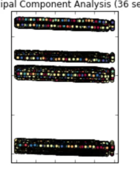
1 Principal Component Analysis of San Francisco Dataset . . . 18
2 Multidimensional Scaling . . . 20
3 From the figure above, an isometric feature is used in the San Francisco Crime Dataset and it performs reasonably well to uncover structure with an execution time approximated to be 2.6 seconds. . . 23
4 Locally Linear Embedding . . . 25
5 Spectral Embedding(Laplacian Eigenmaps) . . . 27
6 Hessian Eigenmaps . . . 30
7 t-Distributed Stochastic Neighbor Embedding (t-SNE) . . . 32
1 MANIFOLD LEARNING
1.1 Introduction
Of the several, non-linear dimensionality reduction techniques known, manifold learning is one of the most effective techniques [1]. A technique that is widely used and one that cuts across various fields of learning including computation, statistics, data mining, data science and geometry, manifold learning has been quite a success. The technique uses manifold algorithms that are based on the idea of several data sets being artificially high [60]. The technique is also applicable in the recovery of low dimensional manifold fixed in a high dimensional area [7]. These manifolds commonly found in high dimensional places can be both non-linear and linear and can be recovered using spectral embedding. Spectral embedding methods involves a set of tools; eigenvectors related to the few eigenvalues located at either the top or bottom of an appropriate matrix [60].
Other than the non-linear methods, there are also linear methods that are equally popular in dimensionality reduction. Two commonly used linear methods include Multi-dimensional scaling as well as the Principal Component Analysis. Of the two the latter is the most popular linear method and even in the linear category as a whole. Other linear methods used include Independent Component Analysis and Project Pursuit. For the former, Non-Gaussianity is maximized in order to identify the data’s linear projections. The latter on the other hand works by engaging in linear projections bound on high dimensional data that are able to put to light specific Non-Gaussian features [60].
The Principal Component Analysis has been used in different fields. In the field of Bioinformatics, the method has been used in a number of ways including gene-expressions experiments that are done on several tissue sources. Also applied in Bioinformatics is multidimensional scaling known as geometry and originally applied in the field of psychology. In the representation of protein structure, multidimensional scaling has been applied [60]. This is done by a combination of accuracy and preci-sion. Much needed information on the function and shape of the protein is gathered from points that are closely positioned [17]. Alternatively in the field of astronomy, supernova remnant images have been analyzed as well as the analysis of galaxies. Additionally, the method is also used in solving problems that involve visualization, compression, data interpolation and denoising [60]. For such problems, approxima-tions are derived and advanced to nonlinear subspaces that are more complicated.
As earlier mentioned nonlinear learning methods are of different categories and can be used in different ways. These nonlinear methods are often considered as local methods whose sole purpose is to maintain the manifold’s local structure found in tiny neighborhoods. Some of the non-linear manifold learning algorithms include but are not limited to Diffusion maps, Locally Linear Embedding, Hessian eigenmaps, Laplacian eigenmaps and Isomap. On the other hand, linear manifold learning works by preserving the manifold’s global structure. In the event that the linear manifold learning does not lead to proper representation of high dimensional data it is then assumed that the data is found along or on the linear manifold. In this case non-linear manifold method is brought into play [7]. Finding real data that accurately lie on a non-linear manifold is not an easy task. For this reason, a comparison is made of
non-linear manifold learning algorithms through the use of simulated data. Simulated data in this case is data that has been drawn from manifolds that contain specific quirks designed in a way possible to reveal the weaknesses of several algorithms [60]. Examples of such data with specific quirks include open box, Swiss roll manifold, fishbowl, sphere and torus. Comparing all the aforementioned methods, there is no single method that can be pointed out to be entirely effective trouncing on all the other methods. However, it has been proven that depending on the situation, some methods come out as better and more effective. With this in mind, the question of the benefit of underlying knowledge on manifold comes up especially when dealing with supervised and unsupervised machine learning algorithms [60]. Should it be based on its closeness to a nonlinear manifold or where the data lies?
1.2 Spaces and Manifolds
Understanding manifolds and the concept of manifold learning can require look-ing at thlook-ings from a different angle. To start with, is to visualize the concept of manifold. “A human looking around at the immediate area would not see the curva-ture of the earth” [8]. This visual representation can act as a perfect guide towards describing what a manifold is. However, we first need to understand that it is from differential geometry as well as topology where the concept of manifold learning is derived from [61]. Curves and figures existing in two and three dimensions are gen-eralized to higher dimension through manifold learning. A manifold can therefore be thought of as topological space with it appearing to be locally flat and also lacking features [61].
1.3 Topological Space
A topological space is nonempty and at the same time a collection of subsets
X that contains arbitrary unions, the space itself, finite intersections of the sets and empty sets [61]. This is what defines topological space. To express it, Topological space takes up the form of (χ, τ), where τ is the representation of the topology that is associated with χ. It is also possible for topological space to be defined in the form of a neighborhood. If a point x is present in a topological space χ then the neighborhood will be in the form of a set with an open set χ [61].
1.4 Topological Manifold
When put to higher levels of dimension, where there is a curved surface that is of three dimensions then it is referred to as manifold learning [62]. A topological spaceM becomes a topological manifold of dimension d. The Hausdorff ensures that differences present in the manifold can be isolated. On the other hand, existence of small local regions at every point means that the manifold will enjoy current conditions of Euclidean space. A 2d+1 space is needed so as to install a d-dimensional manifold [62]. In the form of a topological space it therefore becomes possible for a manifold to take up a topological structure given its in a topological space.
1.5 Riemannian Manifolds
During usual application of a manifold is where calculus can come in and take the form of a smooth manifoldM [63]. This smooth appearance is also known as Rie-mannian Manifolds that is on most occasions defined as a sub manifold. It is deemed to be encompassing Euclidean space, where the ideas of length, bend, and point are safeguarded, also additionally is where smoothness identifies with differentiability. In definition, a topological manifold M can be referred to as a smooth manifold only in the event thatM is continually differentiable to any order [63]. All smooth manifolds are topological manifolds, but the reverse is not necessarily true [8].
1.6 Curves and Geodesics
Connection to an actuated topology means that the Riemannian manifold be-comes a metric space. Additionally, a function dM can be defined as along as the
distance points found on M can be determined using its structure. A curve in M is defined as a smooth mapping from an open interval Ω in R into M [17]. The point
2 DATA ON MANIFOLDS
Among the whole manifold learning calculations that will be talked about, the calculations will assume various finitely many data points,{zi}are arbitrarily chosen
from a smooth t-dimensional manifold M that has a metric of geodesic separation
dM [17]. For this situation, data points are mapped into a higher dimensional space, possibly implicitly.
The purpose of this is to find M as well as identifying an explicit picture of the map ψ given the presence of the available input data xi ∈ X. The application
of these algorithms means that it is possible to have estimates that show us the manifold data reconstructions. Sometimes there exists the problem of impractical visualization purposes. In order to avoid this, only the first two or three points of the coordinate vectors of the reconstructions are taken up and then plotted on a two or three dimensional space [8].
3 LINEAR MANIFOLD LEARNING
A large portion of the factual applications that deals with the issue of dimen-sionality diminishment are chiefly centered on linear dimendimen-sionality lessening and are to some extent referred to as direct complex learning [8]. It is possible to picture a linear manifold as a line, a plane, or a hyper plane. In this case, data is projected into a lower dimensional manifold. Linear manifold learning can be thought of in several ways. The first position is to accept that the information is near a direct manifold, and that the distance from the manifold is dictated by an irregular error [7].
The second option is to consider it a straight manifold really a simple linear ap-proximation to a more complicated type of nonlinear manifold that would probably be a better fit to the data [17]. In both circumstances, the inmate dimensional-ity of the immediate manifold is thought to be a great extent littler than the data dimensionality [8].
The way toward having the capacity to distinguish a direct manifold embed-ded in a higher dimensional space is nearly identifiable capable with the customary estimations issue of direct dimensionality reducing. With different strategies accessi-ble, the recommended strategy for accomplishing direct dimensionality diminishing is to concoct a decreased arrangement of straight changes of the information elements. With direct manifold learning and in addition straight dimensionality lessening, there are various strategies that be used [7]. However In this section, we only portray two linear techniques, specifically, Principal Component Analysis and Multidimensional Scaling. The PCA is considered the most popular dimensionality reduction method, on the other side, multidimensional scaling works by presenting the core element of
the Isomap algorithm for non-linear manifold learning [7].
3.1 Principal Component Analysis
Principal Component Analysis( PCA) is one in a group of methods for taking high-dimensional information, and utilizing the conditions between the factors to have it in a more tractable, lower-dimensional frame, without losing excessive information. The general purpose of PCA are data reduction and interpretation [7].
It is possible to measure the quantity of information found in a random variable through the use of variance also known as the second order property. The Principal Component Analysis therefore becomes the most simple and effective way of reducing the dimensions [8].
As a strategy for dimensionality reduction, PCA has been utilized as a part of lossy information compression, design acknowledgment, and picture analysis [7]. In the field of chemometrics, PCA is utilized as a preparatory stride for building deter-mined factors. This then leads to principal component compression. Additionally, PCA can be used to unearth unusual facets located in a set of data. This can be made possible by plotting the main few sets of key part scores in a scatter plot. With the scatter plot, it then becomes possible to distinguish whether X really is present on a low-dimensional linear manifold of Rr and additionally give assistance recognizing multivariate anomalies, distributional characteristics, and groups of points [8]. In the event that the base arrangement of key segments have variances of close to zero, then this infers those key segments are essentially consistent [7].
Mathematically, PCA are linear combinations of the p random variables
X = (X1, . . . , Xp) (1)
These linear combinations represent the selection of a new coordinate system result-ing from the rotation of the original system with X1, X2. . . , Xp as the coordinate
axes. Principal Components depends on the covariance matrix Σ or the correlation matrix ρ of X1, X2. . . , Xp. The Principal Components are those uncorrelated linear
combinations whose variances are as large as possible. Note that the first PCA is the linear combination with the maximum variance. The figure below is not easy to understand and interpret. Figure 1. Shows Principal Component Analysis applied to San Francisco Crime data.
3.2 Multidimensional Scaling
Multi-Dimensional Scaling (MDS) is as well a traditional approach that maps the first high dimensional space to a lower dimensional space but in a different way [8]. This is done by trying to protect pairwise distances [19]. A helpful inspiration for Multi-Dimensional Scaling can be seen using the following approach. Envision a map of a specific topographical locale, which incorporates a few urban communities and towns. It is normal for such a map to be joined by a two-path table of distances between the chosen pair sets of those towns and cities [18].
However, a big issue with MDS is that it switches that connection between the guide and table that shows the cities proximities. With the method, one is given just the table of vicinities, and the task is to reproduce the map to near likeness [8]. Generally, this is a technique best applied to analyze data similarity or the lack of it. It is important to understand that MDS endeavors to model data similarity or lack of it as separations in geometric spaces. The data can be of different nature.
Data algorithm exists in two forms that aremetric andnon-metric. In the scikit-learn, both are taken into account [48]. In the non-metric form, the calculations will aim at preserving the order of the separations, and therefore look for a monotonic connection between the distances in the implanted space and the dissimilarities. In metric MDS, the info similitude lattice emerges from a metric; the separations between two output points are then set to be as close to the likeness or difference of data. Presence of a monotonic relationship in terms of closeness of two entities as well as the corresponding value similarity and lack of it is the most important thing in Multi-Dimensional Scaling. Despite the fact that there are a few different forms
of Multi-Dimensional Scaling, we depict here just the traditional scaling strategy. Therefore, givenp pointsX1, . . . , Xp ∈Rp from which we compute an (n×n)- matrix
∇= (∇ij) of dissimilarities, where ∇ij = v u u t p X k=1 Xik−Xjk 2 (2)
is the dissimilarity between Xi = (Xi1, . . . , Xip) and Xj = (Xj1, . . . , Xjr), for i, j =
1,2, . . . , p; Squaring and expansion of (2) yields
∇2ij =||Xi||2+||Xj||2−2XiXj (3)
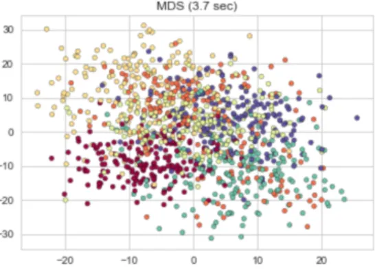
where ||Xi||2 is the squared distance from the point Xi to the origin. The figure
below shows, MDS was successful in unearthing the underlying structure. This in comparison with the Principal Component Analysis shows that MDA does a better job. Even in terms of time, MDA is better with it taking 3.7 seconds for execution while PCA took 36 seconds. Figure 2. Shows Multidimensional Scaling applied to the San Francisco Crime data.
4 NONLINEAR MANIFOLD LEARNING
In this section, we discuss algorithms that have turned out to be exceptionally important in the investigation of non-linear manifold learning [8]. These algorithms includes Diffusion Maps, Local Linear Embedding (LLE), Isomap, Hessian Eigen-maps, Laplacian Eigenmaps and the different forms of Non-Linear PCA. The main objective of nonlinear manifold learning is to recover low dimensional manifold from a high dimensional manifold where most of the linear manifold learning algorithms fails to recover the undelying structure of the manifold [8].
The nonlinear manifold learning embraces simplicity and stays away from opti-mization issues that could create nearby minima. The vast majority of the nonlinear manifold learning algorithms based upon different philosophies regarding how one should recover unknown nonlinear manifolds. However, all algorithms comprise of a three-stage approach with the exception of nonlinear PCA [8].
For the first and third steps, are common to all algorithms [7]. The first step works by step incorporating neighborhood information at each data point to build a weighted diagram that has all the information points as vertices [8]. As for the third step, it is an otherworldly installing venture that includes a (n×n)-eigen equation calculation.
4.1 Isomap
When it comes to Isomap(isometric feature mapping) algorithm, an assumption is made. This assumption is that the smooth manifold M be a convex region of Rs
(s << r) and also that the rooted φ : M → X is an isometry [8]. The concept of
convexity and isometry guides the assumption.
1. Isometry: For any pair of points on the manifold, k, k1 ∈ M, the geodesic
distance between those points equals the Euclidean distance between their cor-responding coordinates [8], r, r1 ∈X which is
∇k,k1 =||r−r1||θ (4)
2. Convexity: Under this concept , it is believed that the manifold M is a convex subset of Rs.
Isomap sees M as an angled area possibly contorted in any number of courses. Notwithstanding, Isomap does not perform well if gaps exist, since this would damage the assumption of convexity [8]. On one hand the isometry assumption gives an im-pression of being sensible under certain circumstance. The presumptions of convexity and isometry are used to come up with a non-linear speculation of multidimensional scaling. Safeguarding geometric properties of the fundamental non-linear manifold is very important. To do so, an approximation is made of the geodesic separations found on the manifold. In this sense, Isomap gives a worldwide approach to complex learning [8]. Isomap algorithm is made up of three stages which are:
1. Nearest-neighbor search : In this case, neighbors are identified for each data points in a high dimensional data space.
2. Compute graph distances : At this stage, the geodesic pairwise differences be-tween all points are calculated.
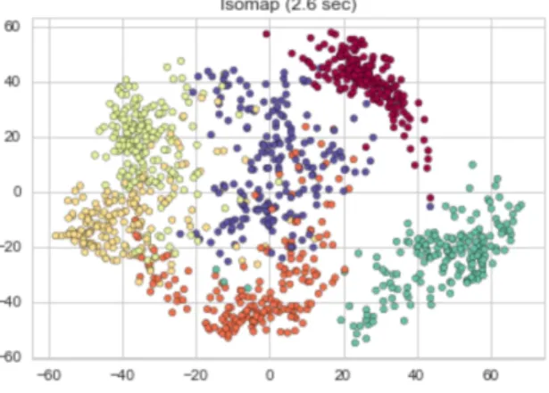
3. Spectral embedding through multidimensional scaling: In order to preserve the distances, data is then embedded through multi-dimensional scaling. Figure 3. Shows Isomap algorithm applied to San Francisco Crime data.
Figure 3: From the figure above, an isometric feature is used in the San Francisco
Crime Dataset and it performs reasonably well to uncover structure with an execution
4.2 Locally Linear Embedding
Local Linear Embedding Algorithm(LLE) can be compared to the Isomap al-gorithm [8]. However, the former’s approach is of a local sense and not worldwide as is the case with the latter. This is because of how LLE strives to preserve near neighborhood data located on the manifold. In a similar fashion, LLE also comprises of three stages which are;
1. Nearest-neighbor search. The execution of LLE depends upon the decision of
K. It is necessary for it to be sufficiently expansive so that the points can be all around reproduced. In addition, it also needs to be sufficiently little for the complex to have little curve. Where the points connecting to a graph remains intact is where LLE is most appropriate. In the event that the connectivity does not exist, the algorithm is then connected independently using the detached sub graphs.
2. Constrained least-squares fits. Reconstructed on Xi can be done by using a
linear function of its K closest neighbors, This leads to
xi = k
X
r=1
λirxr (5)
where λir is a scalar weight for xr with unit sum,
P
rλir = 1, for translation
invariance.
3. Spectral embedding. For determining the weights λi,j the cost function is
min-imized subject to two constraints. Optimal weights λi,j subject to some
so that the objective function will be invariant [8]. Figure 4. Shows the the execution time of LLE, estimated to be 0.85 seconds which is much faster than Isomap algorithm.
4.3 Spectral Embedding(Laplacian Eigenmaps)
The Spectral Embedding algorithm consists of three steps. The algorithm has similarity with the LLE algorithm when it comes to the first and third steps [8]. The three phases of the algorithm include:
1. Nearest-neighbor search: For >0, Nodesiandjare connected if||yi−yj||2 < ,
where the norm is Euclidean norm.
2. Weighted Adjacency Matrix: Choose the weights Λi,j for the weighted adjacency
matrix defined by the heat kernel e−
||xi−yj||2
2σ2 , where scale parameter is σ.
3. Spectral Embedding: Assume graph G is connected. Otherwise proceed with each connected component by computing eigenvalues and eigenvectors for the generalized eigenvector problem. Let∇= (∇ij) be an (n×n) diagonal matrix
and the weight matrix Λ. The (n×n) symmetric matrix Ms =∇ −Λ is known
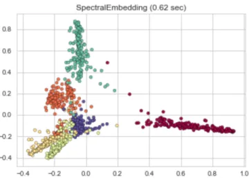
as the graph Laplacian for the graph G. The Laplacian is symmetric, positive semidefinite matrix which can be thought of as an operator on functions defined on vertices ofG. Figure 5. Shows Spectral Embedding algorithm applied to the San Francisco Crime data.
Figure 5: Spectral Embedding(Laplacian Eigenmaps)
4.4 Diffusion Maps
Diffusion maps works on the idea of the Markov Chain [8]. Diffusion map is a kernel method for nonlinear embedding and dimensionality reduction. It was based on the idea of spectral embedding of diffusion affinity kernel, which consists of normalized Gaussian affinities. Euclidean distance in the embedded space approximate diffusion distances in the data. These distances are similar in nature to the geodesic distances used in Isomap, but they are robust to noise. The algorithm just like the previously discussed ones above has three main phases with some steps being almost similar in every way. The three steps are:
1. Nearest-Neighbor Search: Similar to Laplacian Eigenmaps, an integerK is fixed and K-neighborhood is defined. In the same way, Ni denote the neighborhood
2. Pairwise Adjacency Matrix: This is a Gaussian part with width σ; be that different portions might be utilized. For comfort in composition, we will stifle the way that the components of the greater part of the frameworks rely on the estimation e. At that point, Λ = (λi,j) is a pairwise contiguousness network
between n focuses. To make the lattice Λ much more scanty, estimations of its entrances that are littler than some given limit can be set to zero. The graph G = G(V, E) with weight Λ gives data on the nearby geometry of the information.
3. Spectral Embedding: The diffusion probabilities and affinities between X data points can be arranged in (n×n) matrices P and A. P is a stochastic matrix with all row summing equal to one, andA is symmetric. Let A=Q1/2P Q−1/2,
Q is a diagonal matrix. P and Q have the same eigen values and their eigen vectors are also related by Q1/2 and Q−1/2. For t = 2,3, . . . , we have
At=Q1/2PtQ−1/2 (6)
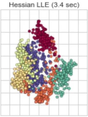
4.5 Hessian Eigenmaps
We can remember that, in specific circumstances, the convexity supposition for Isomap might be excessively prohibitive. In contrast, we may require that the mani-foldM be locally isometric to an open, connected subset ofRs. Well known cases in-clude incorporated groups of articulated pictures that are found in a high-dimensional, digitized picture library [8].
To some degree, finding a fundamental picture complex relies on whether the pictures are sufficiently scattered around the complex and how great is the nature of digitization of each picture? Hessian Eigenmaps were proposed for recouping man-ifolds of high-dimensional libraries of enunciated pictures where the convexity sup-position is frequently abused. Weaker requirements of convexity and isometry then come into play. In this case local isometry and connectedness takes shape [8].
1. Local Isometry: ∆ is a locally isometric embedding of ω intoRs. For any point y0 in a sufficiently small neighborhood around each point yon the manifoldM, the Euclidean distance between their corresponding parameter pointsω, ω0 ∈Ω; that is,
ΛM(y, y0) = ||ω−ω0||ω (7)
where y= ∆(ω) and y0 = ∆(ω0).
2. Connectedness: To recover the parameter vector Ω up to a rigid motion the parameter space is connected to subset Rs.
Figure 6. Shows the The Hessian Locally Linear Embedding (HLLE) method applied to the San Francisco Crime dataset which executes 3.4sec much higher than other algorithms.
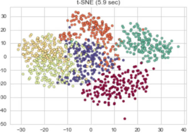
4.6 t-Distributed Stochastic Neighbor Embedding (t-SNE)
t-SNE (TSNE) converts affinities of data points to probabilities [45]. The affini-ties in the original space are represented by Gaussian joint probabiliaffini-ties and the affinities in the embedded space are represented by Student’s t-distributions [46]. This allows t-SNE to be particularly sensitive to local structure and has a few other advantages over existing techniques:
1. Revealing the structure at many scales on a single map .
2. Revealing data that lie in multiple, different, manifolds or clusters.
3. Reducing the tendency to crowd points together at the center.
While Isomap and LLE are best suited to unfold a single continuous low dimensional manifold, t-SNE focuses on the local structure of the data and will tend to extract clustered local groups of samples. This ability to group samples based on the local structure might be beneficial to visually disentangle a dataset that comprises several manifolds at once [45]. The Kullback-Leibler (KL) divergence of the joint probabil-ities in the original space and the embedded space will be minimized by gradient descent. Note that the KL divergence is not convex, i.e. multiple restarts with dif-ferent initializations will end up in local minima of the KL divergence. As a result, it is sometimes useful to try different seeds and select the embedding with the lowest KL divergence [23].
The disadvantages to using t-SNE are :
1. t-SNE is computationally expensive, and can take several hours on million-sample datasets where PCA will finish in seconds or minutes.
2. t-SNE method is limited to two or three dimensional embeddings.
3. The algorithm is stochastic and multiple restarts with different seeds can yield different embeddings. However, it is perfectly legitimate to pick the the embed-ding with the least error.
4. t-SNE global structure is not explicitly preserved. This problem is mitigated by initializing points with PCA [45].
Figure 7. Shows t-Distributed Stochastic Neighbor Embedding applied to the San Francisco Crime dataset.
4.7 Nonlinear PCA (NLPCA)
Nonlinear PCA (NLPCA) is considered as a nonlinear generalization of the di-mension reduction technique Principal Component Analysis (PCA) [8]. NLPCA tries to generalize the principal components from lines(linear) to curves(nonlinear). Neu-ral network with auto-associative architecture is used to achieve this goal. Such auto-associative neural network applies multi-layer perceptron that performs identity mapping ( ie. output of the network should be identical to the input). In the middle of this network, there is a layer which is responsible for the dimension reduction in the data. The question is, how do we generalize PCA to NLPCA?. There are several techniques that have been developed such as Polynomial PCA, Principal Curves and Surfaces, Multilayer Autoassociative Neural Networks, and Kernel PCA [8].
Polynomial PCA: There have been several different attempts made to generalize PCA to data living on or near nonlinear manifolds of a lower-dimensional space than the input space. Higher-degree polynomial transformation of the input variables, and the apply linear PCA, the resulting output is called Polynomial PCA [7].
Principal Curves and Surfaces: A principal curve is a smooth one-dimensional curve that passes through the “middle” of the data, and a principal surface (or prin-cipal manifold) is a generalization of a prinprin-cipal curve to a smooth two- or higher-dimensional manifold [16], and a principal surface (or principal manifold) is a gener-alization of principal curve to a smooth two, three or higher-dimensional space. We can therefore visualize principal curves and surfaces as defining a nonlinear manifold in higher-dimensional input space [8].
whose input layer and output layers are identical and used for nonlinear dimensional-ity reduction. The goal of this method is to perform input dimensionaldimensional-ity reduction in a nonlinear way. This exceptional kind of artificial neural network comprises of more than a five-layer model in which the center three hidden layers of nodes are the mapping layer, the bottleneck layer, and the de-mapping layer, respectively, and each is characterized by a nonlinear activation functions [8].
Kernel PCA: A technique used to generalize polynomial PCA is called Kernel PCA. It’s application expands to support vector machines [58]. This method has 2-stage process :
1. Given input data points nonlinearly transformation of input data into a point in N-dimensional feature space.
2. The second stage solves a linear PCA problem in a feature space which will have a higher dimensionality than that of the input space [8].
5 DATA AND RESULTS
This section entails the application of our manifold learning techniques and ma-chine learning algorithms to the San Francisco Crime Dataset. We applied linear methods like PCA, MDS to the given dataset and non-linear methods like Isomap, Spectral embedding to this same dataset. Table 1. Shows the performance accuracy of each of the machine learning algorithms implemented.
Algorithms Accuracy(Log-Loss)
Random Forest 13.90 Bernoulli Naive Bayes 2.550 Extra Tree 2.497 XGBoosting 2.504
Table 1: Machine Learning Algorithms Performance
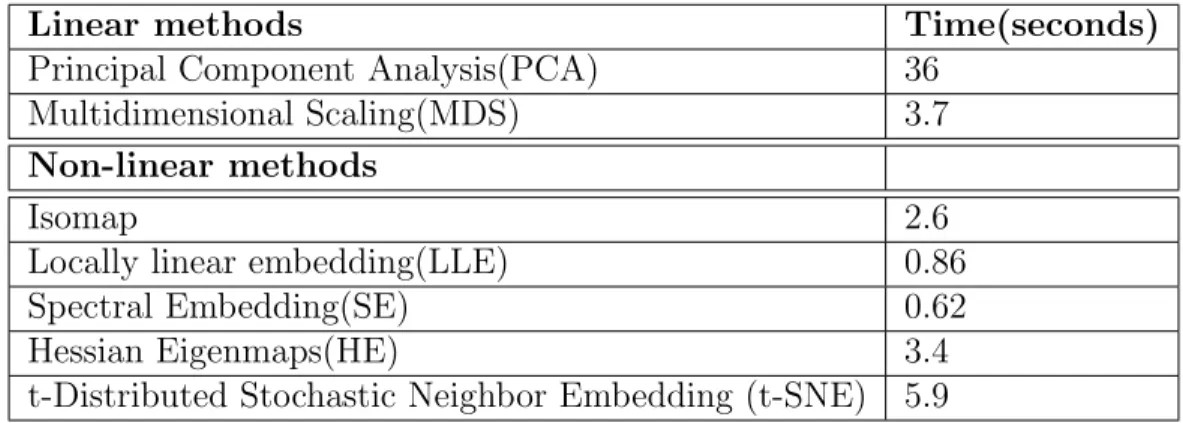
Table 2. Shows the performance metrics of each of the manifold learning techniques implemented.
Linear methods Time(seconds)
Principal Component Analysis(PCA) 36 Multidimensional Scaling(MDS) 3.7
Non-linear methods
Isomap 2.6
Locally linear embedding(LLE) 0.86 Spectral Embedding(SE) 0.62
Hessian Eigenmaps(HE) 3.4
t-Distributed Stochastic Neighbor Embedding (t-SNE) 5.9 Table 2: Manifold Learning Algorithms Performance
We can see from Table 1. Extra Tree was the best algorithm in terms of performance and the worst was Random Forest with log-loss accuracy of 13.90 sec.
was the fasted with execution time of 0.62 sec and the slowest was t-Distributed Stochastic Neighbor Embedding (t-SNE) with execution time of 5.9 sec. However, with linear methods, Principal Component Analysis (PCA) was the worst and the slowest with execution time of 36 sec and Multidimensional Scaling (MDS) did per-form better than PCA with execution time of 3.7 sec. It actually failed to project the data set into a low-dimensional space. The goal of implementing these manifold learning algorithms is speed and accuracy.
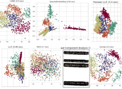
In conclusion, we cannot do better by choosing a better classifier, We can do better by choosing a better dimension reduction method. Figure 8. shows a combined graphs all the manifold learning algorithms implemented.
6 CONCLUSION AND FUTURE WORK
When high-dimensional data, such as those obtained from images or videos, lie on or near a manifold of a lower-dimensional space, it is important to learn the structure of that manifold. Data visualization is an aspect of machine learning and data mining that is gaining attention since data’s insights cannot be achieved without some type of visualization. Dimension reduction is also another aspect that has gained attention in the field of big data ecosystem. We started out applying the usual method of feature engineering and machine learning techniques to the San Francisco Crime Data which only yielded a little above average results. We then applied the various manifold learning techniques to about 878,000 data points and 105 columns. Among these techniques Spectral Embedding was the most efficient and optimal whereasPrincipal Component Analysis was the worst technique. It failed to uncover the underlying structure of the dataset. The entire data set was a sparse matrix due to the feature engineering techniques applied to the original dataset. Again this data set took much memory and space in terms of computations so there should be way to handle this problem in the future. We also made sure the same scale is used over all features. Because manifold learning methods are based on a nearest-neighbor search, the al-gorithm may perform poorly otherwise. The reconstruction error computed by each routine can be used to choose the optimal output dimension.
Future work could be done by applying manifold learning on noisy and/or in-complete data, which is an active area of research.
References
[1] Roweis, Sam T., and Lawrence K. Saul. “Nonlinear dimensionality reduction by locally linear embedding.” Science 290.5500 (2000): 2323-2326.
[2] Ma, Yunqian, and Yun Fu, eds.Manifold learning theory and applications. Chap-ter 1, Pages 1-36, CRC press, 2011
[3] Camastra, Francesco, and Alessandro Vinciarelli. Feature Extraction Methods and Manifold Learning Methods. Springer London, 2008.
[4] Steiner, J. E., et al. “PCA Tomography: how to extract information from data cubes.” Monthly Notices of the Royal Astronomical Society 395.1 (2009): 64-75.
[5] Zheng-Bradley, Xiangqun, et al. “Large scale comparison of global gene expres-sion patterns in human and mouse.” Genome biology 11.12 (2010): 1.
[6] Martinez, Wendy L., et al.Exploratory data analysis with MATLAB. CRC Press, 2010.
[7] Izenman, Alan Julian “Modern Multivariate Statistical Techniques: Regression, Classification, and Manifold Learning” 2008 Springer New York 463–504
[8] Izenman, Alan Julian “Modern Multivariate Statistical Techniques: Regression, Classification, and Manifold Learning” 2008 Springer New York 616–617
[9] Hou, Jingtong, et al. “Global mapping of the protein structure space and ap-plication in structure-based inference of protein function.” Proceedings of the
National Academy of Sciences of the United States of America 102.10 (2005): 3651-3656.
[10] Verleysen, Michel. Learning high-dimensional data. Nato Science Series Sub Se-ries III Computer And Systems Sciences 186 (2003): 141-162.
[11] Cayton, Lawrence. “Algorithms for manifold learning.” Univ. of California at San Diego Tech. Rep (2005): 1-17.
[12] Meurant, Gerard. An introduction to differentiable manifolds and Riemannian geometry. Vol. 120. Academic press, 1986.
[13] Shabir, Muhammad, and Munazza Naz. “On soft topological spaces.” Computers & Mathematics with Applications 61.7 (2011): 1786-1799.
[14] Saul, Lawrence K., and Sam T. Roweis. “Think globally, fit locally: unsupervised learning of low dimensional manifolds.” Journal of Machine Learning Research 4.Jun (2003): 119-155.
[15] Ma, Yunqian, and Yun Fu, eds.Manifold learning theory and applications. Chap-ter 1 Page 4, CRC press, 2011
[16] Hastie, Trevor, and Werner Stuetzle. “Principal curves.” Journal of the American Statistical Association 84.406 (1989): 502-516.
[17] Ma, Yunqian, and Yun Fu, eds.Manifold learning theory and applications. Chap-ter 1, Page 6, CRC press, 2011
[18] Ghodsi, Ali. Dimensionality reduction a short tutorial. Department of Statistics and Actuarial Science, Univ. of Waterloo, Ontario, Canada 37 (2006): 38.
[19] M. Crampin, F. A. E. Pirani Applicable Differential Geometry. Cambridge Uni-versity Press, 1986 Chapter 10 , Page 266.
[20] Kechris, Alexander. Classical descriptive set theory. Vol. 156. Springer Science & Business Media, 2012.
[21] Scholz, Erhard. “The concept of manifold, 1850–1950.” History of topology (1999): 25-64.
[22] Lee, John M. “Smooth manifolds.” Introduction to Smooth Manifolds. Springer New York, 2003. 1-29.
[23] Anderson, T.W. (1963). Asymptotic theory for principal component analysis,
Annals of Mathematical Statistics, 36, 413–432.
[24] Aswani, A., Bickel, P., and Tomlin, C. (2011). Regression on manifolds: estima-tion of the exterior derivative, The Annals of Statistics, 39, 48–81.
[25] Baik, J. and Silverstein, J.W. (2006). Eigenvalues of large sample covariance matrices of spiked population models, Journal of Multivariate Analysis, 97, 1382–1408.
[26] Bai, Z.D. and Silverstein, J.W. (2009). Spectral Analysis of Large Dimensional Random matrices, 2nd Edition, New York: Springer.
[27] Belkin, M. and Niyogi, P. (2002). Laplacian eigenmaps and spectral techniques for embedding and clustering, Advances in Neural Information Processing Sys-tems 14 (T.G. Dietterich, S. Becker, and Z. Ghahramani, eds.), Cambridge, MA: MIT Press, pp. 585–591.
[28] Belkin, M. and Niyogi, P. (2008). Towards a theoretical foundation for Laplacian-based manifold methods, Journal of Computer and System Sciences, 74, 1289–1308.
[29] Bernstein, M., de Silva, V., Langford, J.C., and Tenenbaum, J.B. (2001). Graph approximations to geodesics on embedded manifolds, Unpublished Technical Re-port, Stanford University.
[30] Bourbaki, N. (1989). General Topology (2 volumes), New York: Springer.
[31] Donoho, D. and Grimes, C. (2003b). Hessian eigenmaps: locally linear embed-ding techniques for high-dimensional data,Proceedings of the National Academy of Sciences, 100, 5591–5596.
[32] Kramer, M.A(1991). Nonlinear Principal Component Analysis using autoasso-ciative neural networks, AIChE Journal, 37,233-243.
[33] Freeman, P.E., Newman , J.A., Lee, A.B., Richards, J.W., and Schafer, C.M (2009). Photometric Redshift estimation using spectral connectivity analysis.
[34] Gnanadesikan, R and Wilk, M.B(1969). Data analytic methods in multivariate statistical analysis. In Multivariate Analysis 2 (P.R Krishnaiah, ed) New York: Academic Press.
[35] Goldberg, Y., Zakai, A., Kushnir, D., and Ritov, Y. (2008). Manifold learning: the price of normalization,Journal of Machine Learning Research, 9, 1909–1939.
[36] Ham, J., Lee, D.D., Mika, S., and Scholkopf, B. (2003). A kernel view of the dimensionality reduction of manifolds, Technical Report TR–110, Max Planck Institut fur biologische Kybernetik, Germany.
[37] Kuhnel, W. (2000). Differential Geometry: Curves Surfaces Manifolds, 2nd Edi-tion,Providence, RI: American Mathematical Society.
[38] Lee, J.A. and Verleysen, M. (2007). Nonlinear Dimensionality Reduction, New York: Springer.
[39] Lee, J.M. (2002). Introduction to Smooth Manifolds, New York: Springer.
[40] M. Belkin and P. Niyogi. Laplacian eigenmaps for dimensionality reduction and data representation. Neural Computation, 15(6):1373–1396, 2003
[41] T. Cox and M. Cox.Multidimensional Scaling. Chapman Hall, Boca Raton, 2nd edition, 2001.
[42] L. Saul and S. Roweis. Think globally, fit locally: Unsupervised learning of non-linear manifolds. JMLR, 2003.
[43] J. Friedman T. Hastie, R. Tibshirani. The elements of statistical learning. Springer, New York, 2002.
[44] C. K. I. Williams. On a connection betweenkernel PCA and metric multidimen-sional scaling. Machine Learning, 46(1-3):11–19, 2002.
[45] Van der Maaten, L.J.P.; Hinton, G.Visualizing High-Dimensional Data Using t-SNE Journal of Machine Learning Research (2008)
[46] Van der Maaten, L.J.P.t-Distributed Stochastic Neighbor Embedding
[47] L.J.P. Van der Maaten.Accelerating t-SNE using Tree-Based Algorithms.Journal of Machine Learning Research 15(Oct):3221-3245, 2014.
[48] Pedregosa, F. and Varoquaux, G. and Gramfort Scikit-learn: Machine Learning in Python. Journal of Machine Learning Research , 2011.
http://scikit-learn.org/stable/modules/manifold.html#
[49] Van Der Maaten, L.J.Pt-Distributed Stochastic Neighbor Embedding
http://scikit-learn.org/stable/modules/manifold.html# t-distributed-stochastic-neighbor-embedding-t-sne
[50] Lauren Van Der Maaten, Geoffrey Hinton.Visualizing data using t-SNE
Published 11/08. http://www.jmlr.org/papers/volume9/vandermaaten08a/
vandermaaten08a.pdf
[51] Yeung, K.Y. and Ruzzo, W.L. (2001).Principal component analysis for clustering gene expression data, Human Molecular Genetics, 17, 763–774.
[52] Malthouse ,E.C (1998). Limitations on nonlinear PCA as performed with generic neural networks , IEEE Transactions on Neural Networks, 9 165-173.
[53] Whitney, H. (1936). Differentiable manifolds, Annals of Mathematics, 37, 645–680.
[54] Torgerson, W.S. (1952). Multidimensional scaling: I. Theory and method, Psy-chometrika, 17, 401–419.
[55] Tenenbaum, J.B., de Silva, V., and Langford, J.C. (2000). A global geometric framework for nonlinear dimensionality reduction, Science, 290, 2319–2323.
[56] Spivak, M. (1965). Calculus on Manifolds, New York: Benjamin.
[57] Shawe-Tayor, J. and Cristianini, N. (2004). Kernel Methods for Pattern Analysis, Cambridge, U.K.: Cambridge University Press.
[58] Scholkopf, B., Smola, A.J., and Muller, K.-R. (1998).Nonlinear component anal-ysis as a kernel eigenvalue problem, Neural Computation, 10, 1299–1319.
[59] Nadler, B., Lafon, S., Coifman, R.R., and Kevrekidis, I.G. (2005). Diffusion maps, spectral clustering, and eigenfunctions of Fokker–Planck operators, Neural Information Processing Systems (NIPS), 18, 8 pages
[60] Ma, Yunqian, and Yun Fu, eds. Manifold learning theory and applications. Chapter 1, Pages 1-3, CRC press, 2011
[61] Ma, Yunqian, and Yun Fu, eds. Manifold learning theory and applications. Chapter 1, Page 4, CRC press, 2011
[62] Ma, Yunqian, and Yun Fu, eds. Manifold learning theory and applications. Chapter 1, Page 5, CRC press, 2011
[63] Ma, Yunqian, and Yun Fu, eds. Manifold learning theory and applications. Chapter 1, Page 6, CRC press, 2011
[64] Ma, Yunqian, and Yun Fu, eds. Manifold learning theory and applications. Chapter 1, Page 7, CRC press, 2011
APPENDICES
Listing 1: Sample Python code
import numpy a s np import pandas a s pd from t i m e import t i m e import m a t p l o t l i b . p y p l o t a s p l t from s k l e a r n . c r o s s v a l i d a t i o n import t r a i n t e s t s p l i t from s k l e a r n import c r o s s v a l i d a t i o n from s k l e a r n . c r o s s v a l i d a t i o n import c r o s s v a l s c o r e from s k l e a r n . m e t r i c s import l o g l o s s #e v a l u a t i o n m e t r i c from s k l e a r n import m a n i f o l d from d a t e t i m e import d a t e t i m e
from m a t p l o t l i b . c o l o r s import LogNorm
from s k l e a r n . m e t r i c s import a c c u r a c y s c o r e , c l a s s i f i c a t i o n r e p o r t
from s k l e a r n . d e c o m p o s i t i o n import PCA
from m p l t o o l k i t s . mplot3d import Axes3D
from m a t p l o t l i b . t i c k e r import N u l l F o r m a t t e r
# Next l i n e t o s i l e n c e p y f l a k e s . T h i s i m p o r t i s n e e d e d .
f i g = p l t . f i g u r e ( f i g s i z e =(9 , 1 2 ) )
t 0 = t i m e ( )
pca = PCA( n components =3)
P = pca . f i t t r a n s f o r m (X) t 1 = t i m e ( ) print( ” P r i n c i p a l Component A n a l y s i s : % . 2 g s e c ”%( t 1 − t 0 ) ) ax = f i g . a d d s u b p l o t ( 2 5 9 ) p l t . s c a t t e r (P [ : , 0 ] , P [ : , 1 ] , c=y , cmap=p l t . cm . S p e c t r a l ) p l t . t i t l e ( ” P r i n c i p a l Component A n a l y s i s (%.2 g s e c ) ”%( t 1 − t 0 ) ) ax . x a x i s . s e t m a j o r f o r m a t t e r ( N u l l F o r m a t t e r ( ) ) ax . y a x i s . s e t m a j o r f o r m a t t e r ( N u l l F o r m a t t e r ( ) ) p l t . a x i s ( ’ t i g h t ’ ) p l t . show ( )
VITA
THEOPHILUS SIAMEH
Education: B.S. Mathematics and Computer Science University of Ghana
Legon, Accra, Ghana, 2005-2009.
M.S. Mathematical Sciences East Tennessee State University Johnson City, Tennessee, 2014-2017.
Professional Experience: Data Scientist AC Nielsen
Oldsmar, Florida, 2017-Present.
Data Scientist
Facorne Technologies
Mountain Lakes, New Jersey, 2016-2017.
Graduate Assistant
East Tennessee State University, Johnson City, Tennessee, 2014-2016.
Data Analyst
University of Ghana Graduate School Accra, Ghana, 2009-2010.
Research Interest: Manifold learning, Graph Analytics, Machine learning Data Structures & Algorithm, and Big Data Analytics.