TU Ilmenau | Universitätsbibliothek | ilmedia, 2020
http://www.tu-ilmenau.de/ilmedia
Huang, Jian; Yang, Xu; Shardt, Yuri A.W.; Yan, Xuefeng:
Fault classification in dynamic processes using multiclass relevance vector
machine and slow feature analysis
Original published in: IEEE access / Institute of Electrical and Electronics EngineersNew York, NY : IEEE. - 8 (2020), p. 9115-9123. Original published: 2019-12-24 ISSN: 2169-3536 DOI: 10.1109/ACCESS.2019.2962008 [Visited: 2020-05-11]
This work is licensed under a Creative Commons Attribution 4.0 International license. To view a copy of this license, visit https://creativecommons.org/licenses/by/4.0/
Fault Classification in Dynamic Processes Using
Multiclass Relevance Vector Machine and Slow
Feature Analysis
JIAN HUANG 1,2, XU YANG 1, YURI A. W. SHARDT 3, AND XUEFENG YAN 2
1Key Laboratory of Knowledge Automation for Industrial Processes, Ministry of Education, School of Automation and Electrical Engineering, University of Science and Technology Beijing, Beijing 100083, China
2Key Laboratory of Advanced Control and Optimization for Chemical Processes, Ministry of Education, East China University of Science and Technology, Shanghai 200237, China
3Department of Automation Engineering, Technical University of Ilmenau, 98684 Ilmenau, Germany Corresponding author: Xu Yang ([email protected])
This research was supported in part by the National Natural Science Foundation of China under Grant 61903026 and Grant 61673053, in part by the China Postdoctoral Science Foundation under Grant 2019M660462, in part by the Fundamental Research Funds for the Central Universities under Grant 222201917006, and in part by the National Key Research and Development Program of China under Grant 2017YFB0306403.
ABSTRACT This paper proposes a modified relevance vector machine with slow feature analysis fault classification for industrial processes. Traditional support vector machine classification does not work well when there are insufficient training samples. A relevance vector machine, which is a Bayesian learning-based probabilistic sparse model, is developed to determine the probabilistic prediction and sparse solutions for the fault category. This approach has the benefits of good generalization ability and robustness to small training samples. To maximize the dynamic separability between classes and reduce the computational complexity, slow feature analysis is used to extract the inner dynamic features and reduce the dimension. Experiments comparing the proposed method, relevance vector machine and support vector machine classification are performed using the Tennessee Eastman process. For all faults, relevance vector machine has a classification rate of 39%, while the proposed algorithm has an overall classification rate of 76.1%. This shows the efficiency and advantages of the proposed method.
INDEX TERMS Slow feature analysis, relevance vector machine, dynamic process, fault classification, process monitoring, statistical learning, support vector machine, feature extraction, process control.
I. INTRODUCTION
With the increase in industrial plant complexity, the ability to easily extract information has become more difficult, espe-cially when considering product quality and process safety as critical parameters in the manufacturing process. Data-driven process monitoring techniques have been applied in modern industry to ensure the safety and stability of processes [1]–[8]. In recent years, many multivariate statistical process monitoring algorithms have been proposed for large-scale industrial processes. Heet al. proposed a transition identifica-tion and process monitoring method for multimode processes using a dynamic mutual information similarity analysis [9]. A supervised non-Gaussian latent structure was introduced by Heet al. to model the relationship between predictor and quality variables [10]. He and Zeng proposed double layer
The associate editor coordinating the review of this manuscript and approving it for publication was Gerard-Andre Capolino.
distributed process monitoring based on hierarchical multi-block decomposition for large-scale distributed processes [11]. However, the multivariable statistical methods are not designed for fault classification. Fault detection is used to identify whether the process is under normal condition, but cannot provide any information about the fault type. The main idea of fault classification is to build a classifier on the basis of some known fault categories. Fault classification can provide the connection between the detected fault occurrence and some known faults. Recognizing the type of fault is an important step for process monitoring.
A. CLASSIFICATION METHODS
Numerous machine learning methods have been used for fault classification. Geet al.proposed a kernel-driven semisuper-vised Fisher discriminant analysis (FDA) model for nonlin-ear fault classification, which incorporates the advantages of
J. Huanget al.: Fault Classification in Dynamic Processes Using Multiclass Relevance Vector Machine and Slow Feature Analysis
FDA for fault classification [12]. However, Chiang et al., who investigated the advantages of FDA and support vector machine (SVM), showed that nonlinear SVM outperforms FDA [13]. Jing and Hou studied the multiclass classification problem of SVM and principal component analysis (PCA) [14], while Gao and Hou improved the multiclass SVM using a PCA approach and applied it to the Tennessee Eastman (TE) process [15]. An SVM classifier is the most commonly used classification technique. However, SVM has the following three disadvantages [16], [17]. First, the number of support vectors grows as the size of the training set increases, which also causes the computational complexity to rapidly increase. Secondly, the output from the SVM does not use a probabilis-tic approach for estimating the conditional distribution, which implies that the prediction cannot capture the uncertainty. This means that the accuracy of SVM is sensitive to the train-ing set. Thus, the SVM traintrain-ing set should include a variety of training samples. Thirdly, the classification performance of SVM is sensitive to the parameters. Therefore, a probabilistic and sparse classification algorithm needs to be developed.
Relevance vector machine (RVM) [16], [17] is a classifica-tion method that does not have any of the above limitaclassifica-tions. Given its probabilistic Bayesian framework, RVM can be applied in cases where there are limited training samples. However, no research exists on the application of RVMs to the data-driven fault classification of chemical processes. Considering the sensitivity of the RVM prediction to the input dimension of the training set in industrial data, a sound method should be used to transform the training set into a lower-dimensional feature space, which maximizes the sepa-rability between classes.
B. DYNAMIC DIMENSIONAL REDUCTION METHODS
PCA, a widely used multivariate statistical algorithm, is used to reduce the dimensions. However, PCA is a static dimension reduction method. Sometimes it is necessary to consider the presence of time delay in dynamic systems. In recent years, slow feature analysis (SFA) [18] has been a popular method for extracting dynamic features by focusing on learning the time features that have a slow frequency. Shanget al.pointed out that the time dynamics in the extracted slow features (SFs) is an indicator of process changes [19]. Modified SFA meth-ods have also been proposed [20], [21]. SFA can extract the dynamic representations of the original data from different levels of dynamics. The above studies have shown that SFA can easily extract dynamic features. However, in previous studies, the SFA algorithm was only used for fault detection, which does not provide information about the fault type. In fact, the SFA algorithm has not been applied to fault classification.
C. MOTIVATION FOR THIS PAPER
In modern chemical processes, sufficient training samples for fault classifiers are usually not available, which worsens the performance of traditional classifiers. RVM has the advan-tages of sparsity and probabilistic prediction. It can be applied
when there are insufficient training samples. Furthermore, many chemical processes are large dimensional and have dynamic characteristics. Thus, such processes require that a dynamic dimensional reduction method be used to transform the training set into a lower-dimensional feature space. Since the SFA algorithm shows the inner dynamic characteristics of the faulty samples, it will indirectly increase the classifi-cation performance of RVM. Therefore, it seems plausible to combine SFA and RVM.
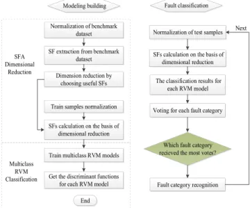
The contributions of this paper are the development of a robust, sparse RVM fault classification method that can be used when there are insufficient training samples and an SFA dimension reduction method that when combined with the RVM classifier can extract the distinct features, and hence, enhance the classification results. This paper proposes a mod-ified multiclass RVM with SFA fault classification strategy for use in industrial processes. First, an SFA dynamic feature extraction model is built on the benchmark data. Then the important features are selected in order to reduce the dimen-sion. After reducing the dimension, the high-dimensional training set is transformed into a low-dimensional dynamic feature space, which decreases the computational complexity of the RVM algorithm. Afterwards, some typical fault sam-ples are collected and used for RVM training. RVM classifies the type of fault, providing a connection between the detected faulty samples and the known faults.
D. NOMENCLATURE
I: Identity matrix
s(t): Slow feature vector
Sk: Selected slow feature matrix
stest: Slow features of the test sample ti: The label for samplei
X: Data matrix
xtest: Testing sample
w: Weight vector
α: Classification parameters M: The number of classes
S: Slow feature matrix
Strain: Training set for RVM ˙
s: First derivative ofs x(t): Input sample
Xtrain: Training set
W: Weight matrix
Wk: Selected weight matrix
h·it: Expectation
II. THEORETICAL BASIS
In this section, the SFA, SVM and RVM algorithms are reviewed. As well, the training results of the SVM and RVM algorithms are compared using a numerical example.
A. SLOW FEATURE ANALYSIS
SFA [22]–[24] extracts the slowly varying features. The input signal is expressed asx(t)=[x1(t),x2(t), . . . ,xm(t)]T. The
optimization objective of SFA is to find a transformation
functiong(x) such that the feature s(t) = g(x(t)) varies as slowly as possible [22], [23]. The function g(x) = [g1(x), g2(x), . . . ,gm(x)]Tis the transformation function, whiles(t)=
[s1(t),s2(t), . . . ,sm(t)]T is the slow feature. The optimization
problem for SFA is
min gi(·) D ˙ s2iE t (1)
with the constraints
hsiit =0 (zero mean), (2) D s2iE t =1 (unit variance), (3) ∀i6=j: sisjt =0 (uncorrelated), (4)
The SFA algorithm is formalized as
s=Wx (5)
whereW is the weight matrix which is expressed asW =
[w1,w2, . . . ,wm]T. The whitening step is carried out by the
singular value decomposition (SVD) of R = x(t)x(t)Tt, which is given as
R=U3UT (6)
The whitening matrix isQ=3−1/2UT. Then, the whitening step is written as
z=3−1/2UTx=Qx (7) Based on (5) and (7), the SF vector is given as
s=Wx=WQ−1z=Pz (8)
whereP = WQ−1. Clearly,zzTt = QxxTQT = I and
hzit =0. Constraints (3) and (4) imply that
D ssTE t =PDzzTE tP T =PPT =I (9)
The optimization problem for SFA is to find an orthogonal matrixPto minimize˙ s2i t, which is given as D ˙ s2iE t =pTi Dz˙z˙TE tpi (10)
The optimal solution is obtained by taking the SVD of the covariance matrix ˙ z˙zT t, that is, D ˙ zz˙TE t =PTP (11) where P is the eigenvector matrix and = diag(λ1, λ2,
. . . , λm) is the eigenvalue matrix, where the eigenvaluesλi
are placed in ascending order. Thus,˙s2it =pT i
˙ z˙zT
tpi=λi.
The weight matrixWis then
W =PQ=P3−1/2UT (12)
B. SUPPORT VECTOR MACHINE
The main idea of the SVM classifier is to find support vectors that define the bounding hyperplanes, so as to maximize the margin between both planes. Let the training set be (xi,ti)
fori=1, 2, . . . ,nandti{−1, 1}, wherexiis theith input
sample andti is the label corresponding to sample xi. The
SVM optimization problem requires solving the optimization problem min1 2w Tw+C n X i=1 ξi ti(wTzi)+b)≥1 −ξi withξi≥0 fori=1,2, . . . ,n (13) where the slack variableξirepresents the violation for
train-ing samplexi. A penalty parameterC is introduced to
con-trol the total violation while maximizing the margin. This introduces a trade-off between maximizing the margin and minimizing the violation. As well, a nonlinear transformation
z = 8(x) is used to project the training data onto a high-dimensional linear space. Based on functional theory, a kernel function should satisfy the Mercer condition.
The Lagrange dual problem is
min α 1 2α T(d˜· ˜dT)α−eTα s.t.:αTt =0, 0≤α≤C (14) whereα=[α1, α2,. . . ,αn]T is the Lagrange multiplier vector
withαi≥0,t=[t1,t2, . . . ,tn]T,d˜ =[t1z1,t2z2, . . . ,tnzn]T,
andeis a unit column vector, that is, a column vector where each entry is 1. The input samplexifor whichαi6=0 is called
a support vector (SV).
The discriminant functionf(x) for a test samplexcan be obtained from f(x)=sign X xi∈SVs αiti8 (x·xi)+b (15)
C. RELEVANCE VECTOR MACHINE
RVM seeks to maximize the possible sparsity, by discarding a large number of extremely small weights and thus, training samples that have no effect on the classification function. Originally, RVM [16], [17], [25], [26] was derived for binary classification. RVM is designed to predict the posterior prob-ability of the membership of the inputx. The training set for RVM is defined as (xi,ti) for i=1, 2, . . . ,n. The learning
function is y(x;w)= n X i=1 ωiK(x,xi)+ω0 (16)
whereK(x,xi) is a kernel transformation andωiis the weight.
Generally, a Gaussian kernel function is used. Bayes’ rule gives the posterior probability ofw, that is,
p(w|t, α)= p(t|w, α)p(w|α)
J. Huanget al.: Fault Classification in Dynamic Processes Using Multiclass Relevance Vector Machine and Slow Feature Analysis
where p(t|w, α) is the posterior probability, p(w|a) is the conditional prior likelihood for the hyperparameters α =
[α1, . . . , αn]T, andp(t|a) is the probability of the evidence.
The logistic sigmoid function σ(y) = 1/(1 + e−y) and Bernoulli distributionp(t|x) are used to generalize the linear model. Thus, (17) can be rewritten as
p(t|w, α)= n Y i=1 σ{y(xi;w)}ti[1−σ{y(xi;w)}]1−ti (18) where t = [t1,t2,· · ·tn]T, ti ∈ {0,1}, and w =
[ω0, ω1,· · ·ωn]T. In (17),p(w|a) is the Gaussian kernel
func-tion, where the weightswiare obtained from the parameterαi
using p(w|α)= n Y i=1 √ αi √ 2π exp −αiw 2 i 2 ! (19)
The approximation procedure is based on Laplace’s method [27], which consists of the following three steps:
1. Given a fixed value ofα,find the maximum posterior weightswMPto provide the location of the mode of the
pos-terior distribution. To solve the problem, the penalized logis-tic log-likelihood function is introduced. Sincep(w|t, α) ∝ P(t|w)p(w|α), the weightswMPcan be obtained from
log{p(t|w)p(w|α)} = n X i=1 tilogyi+(1−ti) log(1−yi)− 1 2w TAw (20)
whereyi=σ{y(xi;w)}andA=diag(α0, α1, . . . , αn).
2. Laplace’s method is used to find a quadratic approxima-tion of the log-posterior based on its mode. Equaapproxima-tion (20) is solved using the second-order Newton optimization method. The Hessian is
∇w∇wlogp(w|t, α)|w
MP = −(8
TB8+A) (21)
where8 = [φ(x1),φ(x2),. . . , φ(xn)]Tis a structure matrix,
in which φ(xi)=[1,K(xi,x1),K(xi,x2),. . . ,K(xi,xn)]T; and
B = diag(β1, β2, . . . , βn) is a diagonal matrix with βi = σ{y(xi)}[1−σ{y(xi)}]. The Hessian matrix is converse and
inverted to give 6 = (8TB8 + A)−1 for the Gaus-sian approximation to the posterior function atwMP. Given
that ∇wlogp(w|t, α)|w
MP = 0, wMP can be written as
wMP =P8TBt.
3. The hyperparametersαare updated using6andwMP αnew i = γi µ2 i (22)
whereγi =1−αi6ii,6iiis the (i,i) diagonal entry of the
matrix 6, andµ = [µ1, . . . , µn]T is the posterior mean
weight vector.
This optimization procedure forces most of theαito
infin-ity, which implies that, based on (19), the corresponding weightswi are discarded. The remaining vectors, which are
called the relevance vectors (RVs), give a sparse solution.
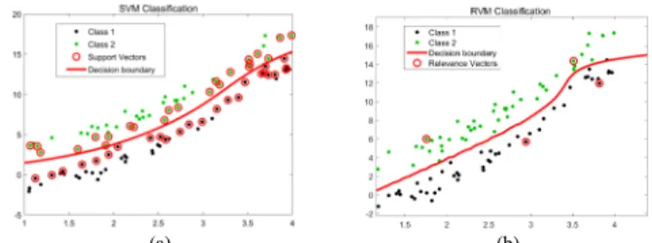
FIGURE 1. Training results for the numerical example: (a) SVM classifier and (b) RVM classifier.
The discriminant functionf(x) can be calculated as
f(x)=
r
X
i=1
wiK(x,xi)+w0 (23)
whereris the number of RVs,xiis the RV, andwirepresents
the remaining weights.
Fault classification usually involves more than 2 classes, whereas RVM and SVM are intrinsically binary fiers. To convert binary classifiers into multiclass classi-fiers, the general strategy is to combine an ensemble of binary classifiers based on some decision rules. In this study, the one strategy is used [17]. In the one-versus-one approach, an ensemble of models, whose training set is made of any two classes is designed. Therefore, the total num-ber of classifiers isM(M −1)/2. When testing an unknown sample, all the discriminant functions need to be calculated. A voting mechanism is used to count the score of each category. The category that obtains the most votes determines the category of the test sample.
D. COMPARISON OF SVM AND RVM USING A NUMERICAL EXAMPLE
Consider the following numerical example with the measure-mentsx=[x1,x2]
x2=x12+ya+v (24)
wherex1is uniformly distributed over the interval [1, 4],νis a
random Gaussian noise with zero mean and variance of 0.25, ais an unmeasurable variable with a uniform distribution over the interval [1, 3], andy{−1, 1} is the label for samplex. The training set consists of 100 samples of which the first 50 samples are labelled 1 and the last 50 samples are labelled
−1.
Figure 1 shows the results of training the SVM and RVM classifiers. The subfigure on the left shows the results for the SVM classifier, while the subfigure on the right shows the same for the RVM classifier. The cir-cled samples represent the support (respectively, relevant) vectors. Comparing the two subfigures, it can be seen that SVM requires 40 support vectors, while RVM only requires 4 relevance vectors. Thus, RVM shows higher sparsity.
III. SLOW FEATURE ANALYSIS AND MULTICLASS RELEVANCE VECTOR MACHINE-BASED FAULT CLASSIFICATION METHOD
Since the number of extracted SFs using the SFA algorithm is always equal to the number of original variables, dimension reduction is required to select an appropriate number of SFs. TheL2-norm method can be used for SF selection. The main
idea of theL2-norm method is that a largeL2norm of a row
inW is assumed to capture more process information. The squared coefficient can be computed using
Li= m
X
j=1
Wij2 (25)
whereWijis the (i,j)-entry of the weight matrixW.
As the training set is chosen randomly from the industrial data set, the correlation between samples may be broken. To extract the inner dynamic features, benchmark data are collected. The normalized benchmark dataset is written asX. The dynamic feature extraction from the dataset Xcan be expressed as Sk = WkX, where Sk is the selected slow
feature matrix and weight matrix is given asWk.
The normalization for both the training set and testing set are based on the normalization of the benchmark data. Assume that the training set is expressed asXtrain. Dynamic
features are extracted to avoid the computational complexity during RVM training. The dimension reduction operation is carried out before RVM training, so that,
Strain=WkXtrain (26)
Similarly, the testing sample xtest can be written as
stest=Wkxtest.
The training set for each binary RVM model can be expressed asS(traini) andStrain(j) , whereS(traini) are the faults with labeliandS(trainj) are the faults with labelj(i 6= j) chosen from the training setStrain. The discriminant functionfij(x) can be
obtained from the RVM training based on (23). Then, the mul-ticlass RVM models are made up of an ensemble of binary RVM classifiers according to the one-versus-one approach.
The multiclass RVM procedure is determined as follows. First, all possible pairs of classifications are built. The total number of binary RVMs isM(M −1)/2. The discriminant functionfij(x) is used to define the assignment of each sample.
The assignments to classes are expressed asP(x,S(traini) ) and P(x,S(trainj) ). A vote is then taken using the vote functionSi(x)
Si(x)= M X j=1 j6=i sgn{fij(x)} (27)
The assignment of the sample to a class is based on the total votes obtained by the class based on the following maximization
C(x)= arg max
i=1,2,...,M
{Si(x)} (28)
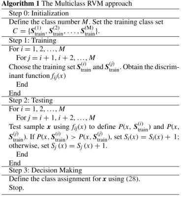
The multiclass RVM approach is summarized by Algorithm 1.
Algorithm 1The Multiclass RVM approach Step 0: Initialization
Define the class numberM. Set the training class set C= {S(train1) ,S(2)train, . . . ,S(M)train}.
Step 1: Training Fori=1, 2, . . . ,M
Forj=i+1,i+2, . . . ,M
Choose the training setS(traini) andS(trainj) . Obtain the discrim-inant functionfij(x) End End Step 2: Testing Fori=1, 2, . . . ,M Forj=i+1,i+2, . . . ,M
Test samplex usingfij(x) to define P(x, S(traini) ) and P(x,
S(trainj) ). IfP(x,S(traini) )>P(x,S(trainj) ), setSi(x)=Si(x)+ 1;
otherwise, setSj(x)=Sj(x)+1.
End End
Step 3: Decision Making
Define the class assignment forxusing (28). Stop.
For the testing vectorstest, the discriminant function set
fij(x) is used to determine the fault category for each binary
RVM classifier. Then, a voting mechanism is used to count the score of each fault category. The test vector belongs to the fault category that obtains the most votes.
Figure 2 shows the flowchart of the SFA-RVM algorithm.
IV. SIMULATIONS AND EXPERIMENTS USING THE TE PROCESS
A. BACKGROUND ABOUT THE TE PROCESS
The TE process was introduced by Downs and Vogel [28]. The control system for the TE process is shown in Figure 3 [29]. There are 22 measured variables and 12 manip-ulated variables for the TE process. There are 500 samples in the normal dataset. To further enhance the TE process, 21 different faults are simulated. For the training dataset, there are 480 faulty samples for each fault. For the testing dataset, the first 160 samples in the faulty dataset are collected under normal condition, while the remaining 800 samples are faulty data. The measurements contain random noise which is carried out using a random seed. The sampling frequency for TE process is 3 minutes. The simulation dataset of the TE is provided at http://web.mit.edu/braatzgroup/links.html. In the fault classification procedure, the training set consists of 100 randomly chosen samples from the training faulty samples for each class.
B. FEATURE EXTRACTION AND DIMENSION REDUCTION OF THE TE PROCESS DATA
The goal of feature extraction is to retain only the most sig-nificant features. The number of SFs retained for dimension
J. Huanget al.: Fault Classification in Dynamic Processes Using Multiclass Relevance Vector Machine and Slow Feature Analysis
FIGURE 2. The flowchart for the proposed SFA-RVM fault classification algorithm.
FIGURE 3. Control strategy for the Tennessee Eastman process.
reduction is based on the L2-norm method. The weight
vectors are re-ordered in descending order based on their L2-norm. The number of slow featureskis determined by
k X i=1 Li/ m X i=1 Li> θ (29)
whereθis the selection threshold.
The number of SFs depends on the data for the cur-rent application. After testing a number of threshold values, the most important SFs are retained when the θ equals to 0.9 with the data used. In the TE process, the number of slow features is 21 according to (29). Figure 4 shows the visualization of the first, second, and third dimensions of the training set. The different categories of fault samples are separated using different colors. Since faults 3, 9, and 15 are commonly considered to be hard to detect, the visualization of the training set does not include faults 3, 9, and 15. The training samples are gathered in a small area and are hardly visually separated. The TE process contains 33 variables
TABLE 1.Fault classification results for the TE process.
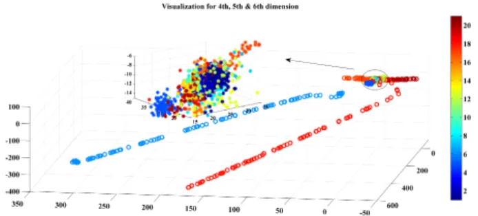
that are combinations of latent factors. The characteristic of high dimensionality makes the classification model complex. Figures 5 and 6 show the visualization for the first 6 dimen-sions of the SFA dimensionally reduced dataset. Compared with Figure 4, part of the faulty samples in the SFA dimen-sionally reduced dataset are visually separated from the other fault categories. The extracted dynamic features max-imize the separation between classes, which highlights the inner dynamic characteristics of faulty samples and indirectly increases the classification performance of RVM.
C. SIMULATION RESULTS
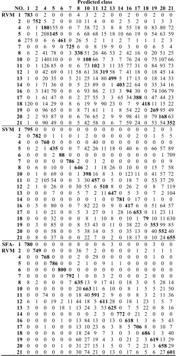
To test the online fault classification performance of the pro-posed method, regular RVM and SVM are used for compari-son. The optimal parameters of the SVM are obtained using cross-validation and the grid search method. Table 1 gives the correct fault classification rate (CFCR) and precision for each fault for RVM, SVM, and SFA-RVM, while Table 2 shows the fusion matrix of the classification results using the RVM, SVM, and SFA-RVM methods for each fault type. Each row gives the fault classification results for a particular fault. The bold numbers on the diagonal show the number of samples that are properly classified. The CFCR is calculated using
CFCR=Number of samples correctly classified
Total number of testing samples (30) The precision for each fault is calculated by
Pr ecision= Number ofsamples correctly classified
Totalnumber ofsamples classified asthisfault (31) In Tables 1 and 2, it can be seen that all three methods have very high correct fault classification rates for Faults 1, 2, and 7. The fault magnitudes for Faults 1, 2, and 7 are large,
TABLE 2. The fusion matrix for fault classification (without faults 3, 9, and 15).
and their distinct fault features make it easy to classify the fault. However, for all methods, the correct fault classification rates for Faults 3, 9, and 15 are very poor. This can be attributed to the fact that these 3 faults have little extractable fault information, which then confuses the fault detection algorithms. The fault classification results for faults without Faults 3, 9, and 15 are also given in Table 1. Furthermore, RVM has a low correct fault classification rate (<30%) for Faults 4, 5, 10, 11, 16, 19, and 20. These faults are conflated with each other, that is, RVM cannot distinguish these faults. Compared with RVM, SVM has better fault classification
FIGURE 4. Visualization of the first, second, and third dimensions of the scaled training dataset.
FIGURE 5. Visualization of the first, second, and third dimensions of the SFA dimensionally reduced training dataset.
results for these faults. However, SVM has poor correct fault classification rates for Faults 6 and 18, where the accuracy is only 10%. The fusion matrix in Table 2 shows that most test samples for Faults 6 and 18 are incorrectly classified as Fault 21. The proposed SFA-RVM algorithm has improved the correct fault classification rates. SFA-RVM achieves the best classification rates for Faults 5, 6, 10, 11, 12, 16, 19, and 20. Of note, the classification rates for SFA-RVM are over 70% for faults excluding Faults 3, 9, and 15 (the last 3 columns in Table 1). Furthermore, the classification rates for Faults 1, 2, 5, 6, and 7 are over 90%. Thus, it has been shown that the proposed SFA-RVM is more robust than RVM and SVM.
Fault 10 is a random variation in the C feed temperature. RVM can hardly recognize fault 10 with low fault classifi-cation rates (approximately 10%). SVM shows better fault classification results. However, the rates are lower than 50%. In the previous fault detection studies, the fault detection rates of some modified process monitoring method for Fault 10 are approximately 0.85 [7], [30], [31]. Some traditional methods such as PCA and DPCA can only detect 50% of the fault samples. The reason why Fault 10 is hard to recognize is that Fault 10 is a random fault, in which the fault amplitude varies considerably. Amplitudes of some fault samples are extremely low, which makes the fault samples similar to the normal samples. Fault detection is a binary classifica-tion problem, which is much easier than fault classificaclassifica-tion, especially for the TE process. The fault classification rate of SFA-RVM (excluding Faults 3, 9, and 15) reaches 0.83, which is close to the best fault detection rate.
Fault 11 is a random change in the reactor cooling inlet temperature. Fault 11 has the same problem as Fault 10 in
J. Huanget al.: Fault Classification in Dynamic Processes Using Multiclass Relevance Vector Machine and Slow Feature Analysis
FIGURE 6. Visualization of the fourth, fifth, and sixth dimensions of the SFA dimensionally reduced training dataset.
TABLE 3. The total classification rates for the TE process.
that it also has low fault amplitudes. The fault classification rates of RVM are 0.11 and 0.13. SVM has better results with a classification rate over 50%. In the previous stud-ies, the fault detection rates of some advanced methods are approximately 0.85 [7], [30], [31]. The fault classification rate of SFA-RVM (excluding Faults 3, 9, and 15) is 0.74. It should be noted that Faults 4 and 11 occurred in the reactor cooling inlet temperature. The only difference between Faults 4 and 11 is that Fault 4 is a step fault whereas Fault 11 is random. Some of the fault samples from Fault 11 are quite similar to samples from Fault 4, which will confuse the fault classification model. It can be seen in Table 2 that there are 74 test samples belonging to Fault 11 that are classified as belonging to Fault 4. In industrial processes, different faults may result in similar evidence because of the presence of the control system. Therefore, the definition of fault categories before model training is also important.
Table 3 shows the overall classification rates for RVM, SVM, decision tree, SFA-based decision tree (SFA-decision tree), and SFA-RVM, as well as the classification rates for different number of training samples (100 and 200 training samples). For all faults (100 training samples), RVM can only recognize 39% of the test samples, while the accuracy of SVM reaches 55.8%. Furthermore, the SFA-RVM algorithm has an overall classification rate of 76.1%, which is the best fault recognition algorithm. The overall classification rates excluding Faults 3, 9, and 15 are higher than those for all faults. The RVM approach leads to a high dimensional solution that causes the accuracy to be lower than 50%. Since SVM is not a probabilistic algorithm, a complete training set is needed to contain enough samples. If the training set is
limited, the accuracy of SVM is sensitive to the size of the training set. For example, some of the TE process faults are random faults, which means that the amplitude of the faults varies. If the randomly chosen training sets differ greatly at different times, the training models of SVM may have many differences. The proposed SFA-RVM algorithm extracts the inner dynamic features to maximize the separability between classes. Dimension reduction avoids the computational com-plexity of the RVM training. The extracted features are good dynamic representations of the TE process. RVM has proba-bilistic prediction and sparsity properties, which achieve good generalization ability and robustness for small scaled training samples. The proposed method takes advantages of both SFA in extracting dynamic features and RVM in classifying.
V. CONCLUSION
In this paper, a modified RVM with the SFA algorithm is pro-posed for fault classification in dynamic industrial processes. SFA extracts the lower-dimensional dynamic features, which maximizes separability and reduces the computational com-plexity of RVM. Simultaneously, a one-versus-one multiclass RVM model is built to recognize the fault category when there are insufficient training samples. RVM classifies the type of faults, providing the connection between the detected faulty samples and known faults. RVM has the advantages of probabilistic prediction and sparsity properties for small training sets. Detailed comparative studies between the SFA-RVM method and traditional SFA-RVM and SVM were carried out using the TE benchmark process. The simulations show that the proposed SFA-RVM method has much better overall fault classification rates than either the RVM or the SVM method alone. For all faults, RVM can only recognize 39%. The SFA-RVM algorithm has an overall classification rate of 76.1%, which is a remarkable improvement.
However, the proposed method was not tested in a real pro-cess. Collecting sufficient data with faults can be an issue for real processes. Furthermore, the knowledge of fault type may be not clear, that is, the training samples for fault classifiers are not available as fast as required. Limited by the diversity and quantity of the training samples for fault classification, the dataset of a realistic experimental application is hard to obtain. Finally, even if faulty data can be obtained, it may not be possible to obtain meaningful fault classifications due to the fact that some of the faults may have a very weak signal. Thus, future work will focus on the application of this method to fault classification on a real process and improving its ability to better handle weak faults.
REFERENCES
[1] Z. Ge, Z. Song, and F. Gao, ‘‘Review of recent research on data-based process monitoring,’’Ind. Eng. Chem. Res., vol. 52, no. 10, pp. 3543–3562, 2013.
[2] S. J. Qin, ‘‘Survey on data-driven industrial process monitoring and diag-nosis,’’Annu. Rev. Control, vol. 36, no. 2, pp. 220–234, Dec. 2012. [3] S. Yin, X. Li, H. Gao, and O. Kaynak, ‘‘Data-based techniques focused on
modern industry: An overview,’’IEEE Trans. Ind. Electron., vol. 62, no. 1, pp. 657–667, Jan. 2015.
[4] V. Venkatasubramanian, R. Rengaswamy, S. N. Kavuri, and K. Yin, ‘‘A review of process fault detection and diagnosis Part III: Process his-tory based methods,’’Comput. Chem. Eng., vol. 27, no. 3, pp. 327–346, Mar. 2003.
[5] S. I. Alabi, A. J. Morris, and E. B. Martin, ‘‘On-line dynamic process monitoring using wavelet-based generic dissimilarity measure,’’Chem. Eng. Res. Des., vol. 83, no. A6, pp. 698–705, Jun. 2005.
[6] Q. Jiang and X. Yan, ‘‘Parallel PCA-KPCA for nonlinear process monitor-ing,’’Control Eng. Pract., vol. 80, pp. 17–25, Nov. 2018.
[7] Q. Jiang, X. Yan, and B. Huang, ‘‘Performance-driven distributed PCA process monitoring based on fault-relevant variable selection and Bayesian inference,’’IEEE Trans. Ind. Electron., vol. 63, no. 1, pp. 377–386, Jan. 2016.
[8] Q. C. Jiang, F. R. Gao, H. Yi, and X. F. Yan, ‘‘Multivariate statistical monitoring of key operation units of batch processes based on time-slice CCA,’’IEEE Trans. Control Syst. Technol., vol. 27, no. 3, pp. 1368–1375, May 2019.
[9] Y. C. He, L. Zhou, Z. Q. Ge, and Z. H. Song, ‘‘Dynamic mutual information similarity based transient process identification and fault detection,’’Can. J. Chem. Eng., vol. 96, no. 7, pp. 1541–1558, Jul. 2018.
[10] Y. He, B. Zhu, C. Liu, and J. Zeng, ‘‘Quality-related locally weighted non-Gaussian regression based soft sensing for multimode processes,’’Ind. Eng. Chem. Res., vol. 57, no. 51, pp. 17452–17461, 2018.
[11] Y. C. He and J. S. Zeng, ‘‘Double layer distributed process monitoring based on hierarchical multi-block decomposition,’’IEEE Access, vol. 7, pp. 17337–17346, 2019.
[12] Z. Ge, S. Zhong, and Y. Zhang, ‘‘Semisupervised kernel learning for FDA model and its application for fault classification in industrial processes,’’
IEEE Trans. Ind. Informat., vol. 12, no. 4, pp. 1403–1411, Aug. 2016. [13] L. H. Chiang, M. E. Kotanchek, and A. K. Kordon, ‘‘Fault diagnosis based
on Fisher discriminant analysis and support vector machines,’’Comput. Chem. Eng., vol. 28, no. 8, pp. 1389–1401, Jul. 2004.
[14] C. Jing and J. Hou, ‘‘SVM and PCA based fault classification approaches for complicated industrial process,’’Neurocomputing, vol. 167, pp. 636–642, Nov. 2015.
[15] X. Gao and J. Hou, ‘‘An improved SVM integrated GS-PCA fault diagno-sis approach of Tennessee Eastman process,’’Neurocomputing, vol. 174, pp. 906–911, Jan. 2016.
[16] M. E. Tipping, ‘‘Sparse Bayesian learning and the relevance vector machine,’’J. Mach. Learn. Res., vol. 1, pp. 211–244, Sep. 2001. [17] F. A. Mianji and Y. Zhang, ‘‘Robust hyperspectral classification using
relevance vector machine,’’IEEE Trans. Geosci. Remote Sens., vol. 49, no. 6, pp. 2100–2112, Jun. 2011.
[18] C. Shang, F. Yang, X. Gao, X. Huang, J. A. K. Suykens, and D. Huang, ‘‘Concurrent monitoring of operating condition deviations and process dynamics anomalies with slow feature analysis,’’AIChE J., vol. 61, no. 11, pp. 3666–3682, May 2015.
[19] C. Shang, B. Huang, F. Yang, and D. Huang, ‘‘Slow feature analysis for monitoring and diagnosis of control performance,’’J. Process Control, vol. 39, pp. 21–34, Mar. 2016.
[20] C. Shang, F. Yang, B. Huang, and D. Huang, ‘‘Recursive slow feature analysis for adaptive monitoring of industrial processes,’’IEEE Trans. Ind. Electron., vol. 65, no. 11, pp. 8895–8905, Nov. 2018.
[21] F. H. Guo, C. Shang, B. Huang, K. C. Wang, F. Yang, and D. X. Huang, ‘‘Monitoring of operating point and process dynamics via probabilistic slow feature analysis,’’Chemometr. Intell. Lab., vol. 151, pp. 115–125, Feb. 2016.
[22] L. Wiskott and T. J. Sejnowski, ‘‘Slow feature analysis: Unsupervised learning of invariances,’’Neural Comput., vol. 14, no. 4, pp. 715–770, Apr. 2002.
[23] L. Wiskott, ‘‘Slow feature analysis: A theoretical analysis of opti-mal free responses,’’Neural Comput., vol. 15, no. 9, pp. 2147–2177, Sep. 2003.
[24] T. Blaschke, P. Berkes, and L. Wiskott, ‘‘What is the relation between slow feature analysis and independent component analysis?’’Neural Comput., vol. 18, no. 10, pp. 2495–2508, Oct. 2006.
[25] A. Widodo, E. Y. Kim, J.-D. Son, B.-S. Yang, A. C. C. Tan, D.-S. Gu, B.-K. Choi, J. Mathew, ‘‘Fault diagnosis of low speed bearing based on relevance vector machine and support vector machine,’’Expert Syst. Appl., vol. 36, pp. 7252–7261, Apr. 2009.
[26] G. M. Foody, ‘‘RVM-based multi-class classification of remotely sensed data,’’Int. J. Remote Sens., vol. 29, no. 6, pp. 1817–1823, 2008. [27] D. J. C. MacKay, ‘‘The evidence framework applied to classification
networks,’’Neural Comput., vol. 4, no. 5, pp. 720–736, Sep. 1992. [28] J. J. Downs and E. F. Vogel, ‘‘A plant-wide industrial process control
problem,’’Comput. Chem. Eng., vol. 17, no. 3, pp. 245–255, Mar. 1993. [29] P. R. Lyman and C. Georgakis, ‘‘Plant-wide control of the Tennessee
Eastman problem,’’Comput. Chem. Eng., vol. 19, no. 3, pp. 321–331, Mar. 1995.
[30] J. Huang and X. Yan, ‘‘Double-step block division plant-wide fault detec-tion and diagnosis based on variable distribudetec-tions and relevant features,’’
J. Chemometrics, vol. 29, no. 11, pp. 587–605, 2015.
[31] Z. Ge and Z. Song, ‘‘Process monitoring based on independent component analysis-principal component analysis (ICA-PCA) and similarity factors,’’