Improved Sampling Based Motion Planning Through Local Learning

(1)

IMPROVED SAMPLING BASED MOTION PLANNING THROUGH LOCAL LEARNING

A Dissertation by

CHINWE PAMELA EKENNA

Submitted to the Office of Graduate and Professional Studies of Texas A&M University

in partial fulfillment of the requirements for the degree of DOCTOR OF PHILOSOPHY

Chair of Committee, Nancy M. Amato Committee Members, J. Martin Scholtz

Dezhen Song Tiffani L. Williams Head of Department, Dilma Da Silva

August 2016

Major Subject: Computer Science

(2)

ABSTRACT

Every motion made by a moving object is either planned implicitly, e.g., human nat-ural movement from one point to another, or explicitly, e.g., pre-planned information about where a robot should move in a room to effectively avoid colliding with obsta-cles. Motion planning is a well studied concept in robotics and it involves moving an object from a start to goal configuration. Motion planning arises in many applica-tion domains such as robotics, computer animaapplica-tion (digital actors), intelligent CAD (virtual prototyping and training) and even computational biology (protein folding and drug design). Interestingly, a single class of planners, sampling-based planners have proven effective in all these domains.

Probabilistic Roadmap Methods (PRMs) are one type of sampling-based planners that sample robot configurations (nodes) and connect them via viable local paths (edges) to form a roadmap containing representative feasible trajectories. The roadmap is then queried to find solution paths between start and goal configurations. Different PRM strategies perform differently given different input parameters, e.g., workspace environments and robot definitions.

Motion planing, however, is computationally hard – it requires geometric path plan-ning which has been shown to be PSPACE hard, complex representational issues for robots with known physical, geometric and temporal constraints, and challeng-ing mappchalleng-ing/representchalleng-ing requirements for the workspace environment. Many im-portant environments, e.g., houses, factories and airports, are heterogeneous, i.e., contain free, cluttered and narrow spaces. Heterogeneous environments, however, introduce a new set of problems for motion planing and PRM strategies because

(3)

there is no ideal method suitable for all regions in the environment.

In this work we introduce a technique that can adapt and apply PRM methods suitable for local regions in an environment. The basic strategy is to first identify a local region of the environment suitable for the current action based on identified neighbors. Next, based on past performance of methods in this region, adapt and pick a method to use at this time. This selection and adaptation is done by applying machine learning.

By performing the local region creation in this dynamic fashion, we remove the need to explicitly partition the environment as was done in previous methods and which is difficult to do, slows down performance and includes the difficult process of determining what strategy to use even after making an explicit partitioning. Our method handles and removes these overheads.

We show benefits of this approach in both planning robot motions and in protein folding simulations. We perform experiments on robots in simulation with different degrees of freedom and varying levels of heterogeneity in the environment and show an improvement in performance when our local learning method is applied. Protein folding simulations were performed on 23 proteins and we note an improvement in the quality of pathways produced with comparable performance in terms of time needed to build the roadmap.

(4)

DEDICATION

God, giving me the strength to finish this journey successfully.

My Dad (In Memory) ”Pay attention to details” really paid off. Thank you Sir. My Mum ”When the time of the fruit comes, it will surely fall”.

My Siblings, giving me something to laugh about irrespective of situations. My Husband Obioma Obim, you make the journey worth it. I love you.

(5)

ACKNOWLEDGEMENT

I would first like to thank my advisor, Dr. Nancy Amato, for mentoring me through the years and teaching me how to get out of my comfort zone. I truly appreciate learning under you.

I would also like to thank my committee members, Dr. J. Martin Scholtz, Dr. Dezhen Song, and Dr. Tiffani L. Williams, for their support and feedback. I appreciate the time taken to help me scale through and streamline my research productively. I would like to thank Dr. Shawna Thomas for taking out time to teach and explain things to me patiently and her interest in my success both personally and academi-cally.

I also thank all the collaborators that I have worked with over the years, both on this work and on other research projects: Diane Uwacu, Hsin(Cindy) Yeh, Mukulika Ghosh, and Jory Denny. I am grateful to have interacted with Cindy and Mukulika through out my graduate studies, striving, encouraging each other and attending conferences together, we had a lot of laughs together. Thank you to all the Parasol members, both former and current.

Thanks to the Schlumberger Faculty for the Future Fellowship for their support during my studies. I would also like to thank the conferences and workshops that provides travel grants for me to participate and present my research findings. These include funding to attend the Grace Hopper Celebration of Women in Computing Conference, the Richard Tapia Celebration of Diversity in Computing, the IEEE/RSJ International Conference on Intelligent Robots and Systems, the IEEE International Conference on Robotics and Automation, and the IEEE International Conference on

(6)

Bioinformatics and Biomedicine.

I would like to thank my family for their steady support. My dad (in memory) who was steadfast in seeing me as worthy of the best and sacrificing to make that happen. My mum, who has sacrificed right from the beginning, time, money, prayers, love, thank you mummy for being your humble self ”The time of nnamma has passed indeed”. My brother Uchenna (in memory), you would have been proud of your little sister. My siblings Nnenna, Ike, Ijeoma, Oke, thank you for making the time fly by with funny anecdotes, words of encouragement and white noise.

Finally, I would like to specially thank my husband Obioma Nwachukwu, your faith in my abilities is astounding, thank you for being patient with me and loving me through it all, I love you dear.

(7)

3. LEARNING FRAMEWORK . . . 25

3.1 Local Learning . . . 25

3.2 Local Learning during Sampling . . . 27

3.3 Local Learning during Connection . . . 29

4. EXPERIMENTS IN ROBOT MOTION PLANNING . . . 31

(8)

4.2 Experimental Setup . . . 32

4.2.1 Single Query Results . . . 33

4.2.2 Multi-Query Experiments . . . 43

5. LOCAL LEARNING AND PROTEIN FOLDING . . . 47

5.1 Related Work and Preliminaries . . . 48

5.1.1 Experimental Protein Dynamics . . . 48

5.1.2 Protein Model . . . 50

5.1.3 PRM for Protein Folding . . . 51

5.1.4 Machine Learning for Protein Analysis and Motion . . . 55

5.2 Learning Framework for Protein Folding . . . 56

5.3 Experiments . . . 57

5.3.1 Learning in Sampling . . . 60

5.3.2 Quality, Time, and the Tradeoff Between Them . . . 62

5.3.3 Learning in Connection . . . 66

5.4 Heterogeneity of the C-Space for Proteins . . . 77

5.4.1 Distance between Parent and Child Configurations . . . 78

5.4.2 Potential vs RMSD and Heterogeneity . . . 79

6. CONCLUSION . . . 82

(9)

LIST OF FIGURES FIGURE Page 1.1 Heterogeneous environments. . . 1 2.1 An illustration of PRM . . . 8 2.2 An illustration of RRT . . . 10 2.3 Heterogeneity . . . 11 4.1 Environments studied. . . 34

4.2 Query time for 2D Heterogeneous for Different Sampling Methods . . 35

4.3 Query time and Frequency of Usage for Different Sampling Methods . 37 4.4 Running time in the 2D Mix Heterogeneous environment using differ-ent local planners averaged over 10 runs. . . 39

4.5 Query time and Frequency of Usage for Different Connection Methods using Bridge Test Sampling Method . . . 41

4.6 Query Time and Frequency of Usage during both phases of PRM construction . . . 42

4.7 Learning in Sampling for the 3D Maze Heterogeneous environment using different local planners averaged over 10 runs. . . 44

4.8 Learning in Connection for the 3D Maze Heterogeneous environment using different local planners averaged over 10 runs. . . 45

4.9 Learning in Both Phases for the 3D Maze Heterogeneous environment using different local planners averaged over 10 runs. . . 46

5.1 Sampling Results over Quality. . . 63

5.2 Sampling Results over Time. . . 64

(10)

5.4 Sampling Results showing Linear Correlation over Time . . . 65 5.5 Cumulative Results for Sampling . . . 66 5.6 Sampling Results Local Use . . . 67 5.7 Local planner success rate for each method over all proteins studied.

The local planner success rate of LLC is greater than all the other methods for 18 of the 23 proteins studied and comparable for 1 of the proteins. Note that entries are ordered by the local planner success rate in the context of LLC. . . 70 5.8 Roadmap quality for each method over all proteins studied. No single

individual connection method performs best across all proteins. LLC produces the best quality roadmaps for 18 of the 12 proteins studied. Note that entries are ordered by LLC performance. . . 71 5.9 Time for each method over all proteins studied. LLC performs as well

as or better than the best performing method for 12 out of 23 proteins studied. Note that entries are ordered by protein length. . . 73 5.10 Time as a function of protein length. LLC and its fastest

competi-tor, Euclidean, display a roughly linear relationship between time and protein length. . . 74 5.11 Difference in time between LLC and its fastest competitor Euclidean. 75 5.12 Cumulative performance of each method over all proteins studied.

Methods are ranked from one (worst) to five (best). Entries are or-dered by cumulative quality ranking. LLC performs better than the other methods across the entire protein set in terms of quality and second best in terms of time. . . 75 5.13 Quality as a function of protein length. LLC outperforms and its

fastest competitor, Euclidean, in terms of quality irrespective of pro-tein length. . . 76 5.14 Connection method usage percentage in LLC across all proteins

stud-ied. Entries ordered by Euclidean usage. . . 77 5.15 Heterogeneity: Difference between the parent and children

configura-tions . . . 79 5.16 Heterogeneity: An α only protein (2ABD) . . . 80

(11)

5.17 Heterogeneity: A β only protein (2CRS) . . . 81 5.18 Heterogeneity: A Mix(α, β) protein (1PGA) . . . 81

(12)

LIST OF TABLES

TABLE Page

4.1 Each method constructs a roadmap until the query is solved. GLS and LLS is comprised of the other 4 sampling methods. All results are averaged over 10 runs. CC is number of connected components present. Boldface entries indicate the most desirable (e.g., shortest running time, Nodes, Edges etc.). . . 36 5.1 Proteins studied. . . 58 5.2 Rigidity Sampling Variants used . . . 59 5.3 Learning in Sampling:Validation of secondary structure formation

or-der to experimental data when available. Proteins are oror-dered by protein length as in Table 5.1. . . 61 5.4 Learning in Connection:Validation of secondary structure formation

order to experimental data when available. Proteins are ordered by protein length as in Table 5.1. . . 68 6.1 Lessons Learned . . . 82

(13)

1. INTRODUCTION

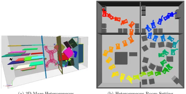
Planning motions is needed in many disciplines such as planning for deformable robots [42,86,94], manipulation planning [55], computational biology search problems [81, 102], character animation for games and movies, and virtual prototyping. A motion planner finds a valid sequence of motions, or path, for a robot to transit from an initial state to a goal state or reports that no such path exists. The robot can be any movable system: an articulated arm in a factory, a car, or a protein. Robots or objects most often have to plan and navigate in heterogeneous environments, i.e., containing a combination of free spaces, narrow tunnels and obstacles. Environments as shown in Figure 1.1 are heterogeneous because robots at different positions would have varying visibility of the entire space. These robots also have different complexity ranging from rigid bodies to highly articulated linkages with many degrees of freedom.

(a) 3D Maze Heterogeneous (b) Heterogeneous Room Setting

(14)

Various motion planning methods have been developed to solve this problem but no single planner is scalable to all environments and this could be due to a number of reasons. One reason is that the heterogeneity of the environment is not investigated and so the environment is seen as homogeneous [16, 29] which our research shows is not always the case and affects performance. Another reason is the concentration of research to a specific robot type and type of environment which limits the use of these methods across other environments [2, 8, 52].

Previous work looked into explicitly partitioning the environment and then applying different methods in the different partitions. However, this is difficult to do due to the challenge of identifying when the environment has been broken into homogeneous pieces or determining if the right method has been applied [83, 100]. Our method addresses this issue by dynamically creating regions and uses machine learning tech-niques to select the appropriate methods to apply based on information regarding their past performance in that local region. Thus we remove the need to explic-itly partition or know beforehand what method is suitable in different parts of the environment.

1.1 Research Contributions

The goal of this research is to develop a means to dynamically create regions in heterogeneous environments, access stored information about the performance of methods in these identified regions, and then intelligently decide what method is most suitable during the current iteration. This research focuses on Probabilistic Roadmap Methods (PRMs) [58]. PRMs are state of the art motion planning algo-rithms that solve motion planning problems in two phases. During the sampling stage, valid configurations of the robot in the environment are generated, and

(15)

dur-ing the connection stage those sampled nodes are connected together with edges to construct a roadmap that is used to find the valid path. We study characteristics peculiar to different probabilistic planners in a bid to utilize their usefulness when needed in these different motion planning scenarios.

We utilize reinforcement learning approaches to intelligently decide which PRM method to apply in the local region and the current iteration during roadmap con-struction. Our technique extends different algorithms such as the multi-arm bandit problem [11, 20, 99]. We include a localizing feature that keeps the learning sensitive to regions in the environment with similar characteristics, and which enables learning from past experience of the methods in these regions so that methods most suitable for the current iteration can be selected. By applying learning in these dynamically determined regions, we remove the need to explicitly partition environments and the overhead of deciding which method to use for a given input problem.

Our results show that we either achieve improved performance or at the least com-parable performance with the best single planning method. We test on a variety of heterogeneous environments and study the performance of our learning based ap-proach. We compare the performance of local learning to global learning (no local region identification).

Our results show our framework is able to make improvements on the roadmap quality and to solve the query problems in less time than other non-learned scenarios in most cases.

The main contributions of this research include the following:

• A local region feature created on the fly that localizes learning to areas of interest and based on past performance applies suitable methods in the current

(16)

locale and iteration.

• A machine learning reward based technique that locally rewards the perfor-mance of these methods.

• A technique that utilizes the strengths of these PRM methods while minimizing their weaknesses (use when and where needed).

Portions of this research have been previously published and presented. The basic ap-plication of learning to PRM was presented at IEEE/RSJ International Conference on Intelligent Robots and Systems (IROS) in 2013 [35]. Improvements on the learn-ing strategy and introduction of the local region feature was presented atIEEE/RSJ International Conference on Intelligent Robots and Systems (IROS) in 2015 [37]. A discussion and investigation on the application of local learning to the different phases of PRM roadmap construction was presented at The Machine Learning in

Planning and Control of Robot Motion Workshop (IROS-MLPC) in 2015 [39].

Ap-plication of local learning to protein folding was presented atThe IEEE International Conference on Bioinformatics and Biomedicine (BIBM) in 2015 [36].

1.2 Outline

Chapter 2 discusses some important primitives and background on motion planning methods and the multi-arm bandit problem algorithm, and then discusses some re-lated work on sampling methods, connection methods, and adaptive learning strate-gies employed to solve the motion planning problem. Chapter 3 describes our learning framework and the algorithms developed. Chapter 4 discusses our local learning ap-proach showing experiments we performed when applied to sampling and connection separately and then investigates what happens when applied to both sampling and connection. Chapter 5 shows an application of local learning to proteins, studying

(17)

different protein folding simulations and the application of our method to the sam-pling and connection stages. We finally conclude and discuss future work in Chapter 6.

(18)

2. PRELIMINARIES AND RELATED WORK

In this section we discuss some motion planning primitives, and sampling based mo-tion planning algorithms including graph based and tree based methods. We further describe reinforcement learning techniques applicable to our framework, PRMs, exist-ing samplexist-ing methods, existexist-ing connection methods and machine learnexist-ing strategies applied to motion planning.

2.1 Motion Planning

The motion planning problem involves finding a valid path (e.g., collision-free and satisfying all joint limit and/or loop closure constraints) for a movable object starting from its start configuration to a goal configuration in an environment [24]. A single configuration is defined based on the movable object’s d independent parameters or degrees of freedom (dof). The set of all possible configurations (both feasible and

infeasible) defines a configuration space (C-Space) [24, 91]. C-Space is partitioned into two components: C-free (the set of all feasible configurations) and C-obst (the set of all infeasible configurations). Motion planning then becomes the problem of finding a continuous sequence of points in C-free that connects the start and the goal configuration.

A complete solution to the motion planning problem is known to be computationally expensive and it has been shown that this problem is PSPACE-hard with an upper bound that is exponential in the number of the movable object’s dofs [24, 91].

Basi-cally, any planner that is guaranteed to find a solution or determine that none exists requires exponential space that is in the the number of DOFs. Heuristic and approx-imate algorithms were therefore implemented that trade completeness for efficiency

(19)

and sampling-based motion planning is one such approach.

2.1.1 Sampling Based Motion Planning

Sampling-based methods [24] are a state-of-the-art approach to solving motion plan-ning problems. These methods are known to be probabilistically complete because even though there is no guarantee to find a solution if one exists, the probabil-ity of finding a solution if it exists increases as the number of samples generated also increases. Sampling-based methods are broadly classified into two main classes: graph-based methods such as the Probabilistic Roadmap Method (PRM) [58] and tree-based methods such as Expansive-Space tree planner (ESTs) [47] and Rapidly-exploring Random Tree (RRT) [65].

2.1.1.1 Graph-Based Methods

Probabilistic RoadMaps (PRMs) [58] are sampling-based motion planning approaches that use a two stage process to solve planning problems: roadmap construction and query processing. During roadmap construction, PRMs sample the configura-tion space (C-Space), i.e., the set of all possible robot placements, retaining valid ones as roadmap nodes, and attempting to connect them using some local planner (e.g., straightline). PRM solves motion planning problems by constructing a graph G = (V, E), called a roadmap, to show how connected C-free is (Figure 2.1 [3]). PRMs have been shown to be probabilistically complete [57].

The basic PRM [58] (shown in Algorithm 1), begins with generating nodes using uniform random sampling and then attempts connections between a node and its k-nearest neighbors as computed using some distance metric (e.g., Grid based, Root-Mean-Square or Euclidean distance [5]). Once the roadmap is constructed, query processing is done by connecting the start and goal configurations to the roadmap

(20)

Figure 2.1: An illustration of PRM∗

and extracting a path from the roadmap that connects them. Many variants of PRMs have been proposed that bias node generation or connection or query processing in various ways to handle instances such as narrow corridors or obstacles too close to the boundary; we discuss some of these variants in Section 2.3.

2.1.1.2 Tree-Based Methods

The Expansive Space Tree Planner (ESTs) and Rapidly-exploring Random Tree (RRT) are two common tree based methods in sampling based motion planning. These methods are most commonly used in solving single query problems. Specif-ically, RRT is particularly well suited for non-holonomic and kinodynamic motion planning problems [66, 67]. RRT (shown in Algorithm 2 and illustrated in Fig-ure 2.2 [3]) grows a tree rooted at the start configuration and expands towards unexplored areas of the C-Space. RRT begins by generating a uniform random sam-ple qrand, and identifies the closest node qnear in the tree to qrand, and then qnear is “extended” toward qrand for a stepsize of at most ∆q. If the extension is successful, qnew is added to the tree as a node and the pair qnear and qnew is added as an edge.

∗_{Reprinted with permission from ”Improving the Connectivitiy of PRM Roadmaps” by Marco}

Morales, Samuel Rodriguez, Nancy M. Amato, 2003 IEEE International Conference on Robotics and Automation (ICRA), pp. 4427-4432 [82] c2003 IEEE.

(21)

Algorithm 1 Basic PRM

Input. An environment env, number of nodes N

Output. A roadmap graph Gcontaining N valid nodes connected

1: i←0 2: while i < N do 3: q← GetRandomValidNode(env) 4: G.AddNode(q) 5: i←i+ 1 6: end while 7: for all q ∈G do 8: Q← FindNeighbor(G, q, k)

9: for all qnear ∈Qdo

10: if local planner can connect q and qnear then 11: G.AddEdge(q, qnear)

12: end if

13: end for

14: end for

15: return G

To solve a particular query, RRT repeats this process until the goal configuration is connected to the tree. RRT-connect is a variant that grows two trees towards each other; one rooted at the start configuration and the other at the goal configura-tion [59]. These two trees explore C-Space until they are connected. Many variants of RRT have been proposed and discussed [15, 24, 32, 51, 56, 80, 93].

2.1.2 Heterogeneity of the C-Space

Dale and Amato in [28] made some interesting analysis in defining the heterogeneity of a space. They defined four characterizing measures to help determine when a region of the C-Space is heterogeneous. They classify a region of the C-Space based on the ratio of non-colliding nodes to all nodes sampled. If this ratio is one, then the

†_{Reprinted with permission from ”Adapting RRT Growth for Heterogeneous Environments” by}

Jory Denny, Marco A. Morales A., Samuel Rodriguez, Nancy M. Amato, 2013 IEEE International Conference on Intelligent Robots and Systems (IROS), pp. 1772 - 1778 [33] c2013 IEEE.

(22)

Figure 2.2: An illustration of RRT†

Algorithm 2 Basic RRT

Input. An environment env, a root qroot, the number of nodes N

Output. A tree T containing N nodes rooted at qroot 1: T.AddNode(qroot)

2: i←0

3: while i < N do

4: qrand ← GetRandomNode(env) 5: qnear ←FindNeighbor(T, qrand,1) 6: qnew ← Extend(qnear, qrand)

7: if !TooSimilar(qnear, qnew) ∧ IsValid(qnew) then 8: T.AddNode(qnew)

9: T.AddEdge(qnear, qnew) 10: i←i+ 1

11: end if

12: end while

13: return T

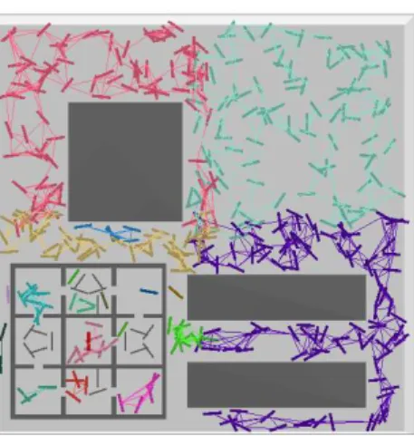
region is free, C-free . If the ratio equals zero, then the region is blocked, C-obst. Another metric they used to define the workspace is based on the number of con-nected components and the number of nodes present (size) in a concon-nected component (CC). Figure 2.3 shows an example environment with a mixture of free and cluttered

(23)

Figure 2.3: Heterogeneity

regions. Using the ratio method it becomes hard to make an informed decision about the C-Space and how heterogeneous it is. In a free space, the CC will be 1 and the size of the CC will include all valid nodes. As the number of CC increases and the size of the CC reduce then we identify more cluttered regions. This difference helps characterize the right top half of the figure as free and the remaining as cluttered. The final metric they discuss relates to defining obstacles in the workspace. They de-termine anobstaclebased on the ratio of surface connection and surface connections attempted as seen in Figure 2.3. This inclusion of the surface was based on research in [8, 17] that observed that given that nodes can be obtained arbitrarily close to configuration obstacle surfaces, the results of connection attempts between nodes near the surface of an obstacle can be used to provide a surface characterization for the obstacle.

Given this characterization, we define a heterogeneous C-Space as containing more than one type of region – free space, cluttered or obstacle regions.

(24)

2.2 Reinforcement Learning

Reinforcement learning is a machine learning concept that involves learning what actions to take in a given scenario to maximize a cumulative reward. This learning concept focuses on utilizing exploitation and exploration techniques.

Exploitation involves continually using the best available methods while exploration continually looks for better methods from the list that could potentially be exploited. Balancing when to explore or exploit is an open research question that has been studied for decades. In our work we utilize one of the standard approaches called the multi-arm bandit problem.

2.2.1 Multi-arm Bandit Problem

In this section we describe the reinforcement learning approach called the multi-arm bandit problem which is an important primitive we employ in our work.

The Multi-armed bandit problem (MAB) was first presented by Robbins [63] and provided a platform for modeling how automated agents gain new knowledge when exploring their environment. This is done by exploiting currently reliable knowledge about the environment at a particular point in time. MAB is a reinforcement learning strategy that investigates the trade-off between exploration and exploitation.

A common analogy of the MAB problem is that of a gambler with multiple slot machines, the gambler keeps playing the hand that is winning (exploitation) while looking out for other slots when they become a winning hand.

As a stochastic approach, the bandit problem consists of a set of K probability distributions (P1, ..., PK) with associated expected values (ϕ1, ..., ϕK) and variances (σ2

(25)

These probability distributions generally correspond to the arms for a slot machine and the player is viewed as a gambler with a goal of winning as much money as possible by pulling all these arms as much as possible.

At each iteration, t= 1,2, ..., the player selects an arm, with index j(t), and receives a rewardr(t)∽Pj(t) . The player has a two-fold goal: on one hand, identify quickly the winning hand; on the other hand, improve on the rewards collected as much as possible while playing. Bandit algorithms specify a strategy by which the player should choose an arm j(t) at each turn [61].

A popular performance measure for bandit algorithms is the total expected regret, the regret is how much worse the algorithm performs as opposed to the best experts decisions.

The regret T is calculated as: RT =T ϕ∗− T

X

t=1

ϕj(t) where ϕ∗ =maxi=1,...kϕ1 is the expected reward from the best arm [20].

The payoff of the algorithm at step t is defined as the number of correct guesses minus the number of wrong guesses.

2.3 Related Work

In this section we discuss relevant work that has been done in the field of sampling based planning both during sampling and connection. We include discussions about adaptive methods that have been employed in all these cases as well.

2.3.1 Existing Sampling Methods

Considerable effort has been dedicated to finding ways of increasing sampling in narrow and difficult regions of environments. In this section we look at some of the most successful strategies and their individual strengths and limitations.

(26)

• Uniform

1. Uniform Sampling [58]: This method generates nodes uniformly at ran-dom in C-Space retaining valid ones. A drawback with this approach is its inability to sample narrow passages efficiently thus increasing the chances of oversampling in open areas.

• Near Obstacles

1. Obstacle-Based PRM (OBPRM) [7, 8]: samples configurations near C-obst surfaces by pushing configurations to the C-C-obst boundary. Even if OBPRM excels in narrow passages, it can be expensive because it requires many validity tests. In addition, the nature of its sampling tends to produce paths with low clearances.

2. Gaussian PRM [17]: This technique attempts to generate configurations that are a Gaussian distance d away from the obstacle surfaces. A first configuration is randomly generated and the second one is generated a Gaussian distance d away from the first configuration, where d is a user-specified parameter. If the validity of the two configurations differ, the valid one will be retained as a node in the roadmap. Otherwise, both are discarded. This method’s performance is dependent on tuning the parameter d for each environment.

3. Uniform OBPRM (UOBPRM) [25]: uses the uniform sampling framework to generate uniformly distributed configurations near C-obst surfaces by detecting when C-obst surfaces have been crossed. This is done by look-ing for validity changes between consecutive points along a defined line segment d. When a validity change occurs, the valid sample is retained

(27)

as a roadmap node. This method also needs some parameter tuning on d to get effective results.

• In Narrow Passages

1. Bridge Test PRM [46]: This method was implemented to boost sampling density in narrow passage to improve the connectivity of roadmaps. In a bridge test they check for collision at three sampled configurations: the two endpoints and the midpoint of a short line segment. This method also suffers from parameter tuning which can greatly affect the performance and quality of the mappings produced.

2. Toggle PRM [29,31]: performs a coordinated mapping of both free and C-obst. It retains witnesses from failed connection attempts in one space to augment the roadmap in the opposite space. [31] provides a novel classi-fication of narrow passages that can be solved efficiently by this method-ology. Toggle PRM is able to solve certain narrow passages, but it does not provide a guarantee on the solution quality.

3. Medial Axis PRM(MAPRM) [71, 108]: Medial Axis PRM was proposed to generate configurations along the medial axis of C-free to increase the path clearance. The medial axis is a set of points that are equidistant to two or more obstacles and are guaranteed to have maximal clearance. The medial axis is a strong deformation retraction which makes a one-to-one mapping between every point in C-Space and the corresponding point on the medial axis and is thus a useful construction for motion planning. It makes use of fundamental primitives which are computation of penetration depth and clearance in C-Space to achieve this. However, MAPRM does not provide any guarantee regarding the distribution of samples along the

(28)

medial axis and it is expensive to produce samples.

4. Uniform MAPRM(UMAPRM) [109]: UMAPRM generates uniformly dis-tributed samples along the medial axis by checking the closest obstacle changes between two neighboring configurations on the segment. The medial axis is crossed when there is a closest obstacle change. A binary search finds and retains the configuration on the medial axis.

2.3.2 Existing Connection Methods

Connection methods are primitives used in PRM to connect nodes via edges together while building a roadmap. The connection method defined within our context in-clude a combination of a distance metric (used to calculate the distance between configurations), a neighbor finding approach (to identify pairs of ”close/similar” con-figurations), and a local planner (to determine if a feasible path exists between two configurations). In this section we discuss these three primitives used during the connection phase for PRMs, i.e., neighbor finding methods, distance metrics and local planners.

• Distance Metrics

A distance metric is a function δ that computes some “distance” between two configurations a = ha1, a2, . . . , adi and b = hb1, b2, . . . , bdi, i.e., δ(a, b) → R, where d is the dimension of a configuration. A good distance metric for a PRM predicts how likely it is that a pair of nodes can be connected. In this research, we study the set of distance metrics commonly used in PRMs:

(29)

dimensions:

δ(a, b) =p(a1 −b1)2+ (a2−b2)2+· · ·+ (ad−bd)2

2. The scaled Euclidean distance metric is a variant

δ(a, b) =ps(pos mag)2_{+ (1}₋_{s)(ori mag)}2

where pos mag is the Euclidean distance of the positional dimensions, ori mag is the Euclidean distance of orientational dimensions, and s is a weighting parameter. In the results presented here, we use s = 0.5 and refer to this as “Euclidean”.

3. Minkowski: The Minkowski distance is the generalized form of the Eu-clidean distance which uses parametersr1,r2, andr3 to specify the expo-nents and roots used:

δ(a, b) = rq₃

(a1 −b1)r

1

+· · ·+ (ad−1−bd−1)r

2

The positional DOFs (usually the first 3 dimensions) use r1 as a power factor and the orientation/joint DOFs user2 as a power factor – typically, r1 =r2 and r3 = 1/r1.

4. Manhattan: The Manhattan distance metric is the distance between two points if a grid path is followed:

δ(a, b) = (|a1−b1|+|a2−b2|+· · ·+|ad−bd|)

(30)

distance between two objects X and Y. It records the level of similarity between the position and orientation of two objects:

δ(X, Y) =

r

(X1−Y1)2+ (X2−Y2)2+. . .+ (Xd−Yd)2 d

6. Swept Volume: Swept volume is the volume generated by the continu-ous motion (translation and/or rotation) of a geometric object through space. The swept volume distance is the volume swept by the robot while following the motion prescribed by the local planner. For an articulated linkage, this becomes the sum of the swept volumes of each of the links. This distance metric is expensive but more accurate for any local planner. • Neighbor Finding Methods

1. K-Closest /R-Closest methods: These methods return thekclosest neigh-bors to a node based on some distance metric, where k is normally some small constant, and can be done in logarithmic time. The advantage is that nodes are more likely to be connectable by the local planner because the volume of C-Space the connection occupies is smaller. Another ap-proach is ther-closest method which returns all neighbors within a radius r of the node as determined by some distance metric. Here, the size of the neighbor set is not fixed but is dependent on the sampling density. 2. Randomized K-Closest variants: Two randomized variants of these

meth-ods are proposed in [78]: Closest,Rand and R-Closest,Rand. K-Closest,K-Rand randomly selects k neighbors from the k2 closest nodes, where typically k2 = 3k. R-Closest,K-Rand selects k random neighbors from those within a distance r. In some cases, these methods outperform

(31)

K-Closest as they introduce some useful randomness.

3. Reachablility Based Analysis [43]: This work describes the properties of these neighbor finding approaches and motivates research on connections based upon reachability analysis. However, these are expensive and should be limited to acquiring roadmap connectivity and/or seeking asymptoti-cally shortest paths [56].

4. Metric Trees [104]: These data structures organize the nodes in a spatial hierarchical manner by iteratively dividing the set into two equal subsets resulting in a tree with O(logn) depth. However, as the dataset dimen-sionality increases, their performance decreases [72].

5. KD-trees [10]: These trees extend the binary tree into a D-dimensional data structure which provides a good model for problems with high di-mensionality. However, a separate data structure needs to be stored and updated each time a node is added to the roadmap.

6. Approximate Neighbor Finding Methods

These methods address the running time issue of exact neighbor finding approaches by instead returning a set of approximate K-Closest neighbors. These include spill trees [72], MPNN [110], and Distance-based Projection onto Euclidean Space [90]. These methods usually provide a bound on the approximation error.

• Local Planners

A local planner (LP) connects two nodes with an edge based on defined close-ness characteristics [5]. There are many local planners that can be used to connect two nodesaand b, and in this work we focus on two: StraightLine and

(32)

RotateAtS. We used the StraightLine local planner because apart from being commonly used, it is the fastest to compute and thus has less computation overhead. RotateAtS is useful as a comparison tool because it is an offshoot of the straightline local planner but does some rotation along the way. We also briefly describe other local planning methods called TransformAtS and Toggle LP.

1. StraightLine [5]: interpolates between two points in C-Space checking intermediate points on a straight line in C-Space. Although this local planner is simple and fast, it often fails in cluttered environments where nearest neighbors cannot be connected by a straight line due to the large swept volume.

2. RotateAtS [5]: reduces the swept volume by translating from a for some distance s toward b, changes all orientation DoFs, and translates again to get to b. The rotation allows the local planner some chance to get around obstacles making it more successful with samples that are close to obstacles.

3. TransformAtS is a modification of RotateAtS that changes all DOFs one by one when it gets tos.

4. Toggle LP [30]: a straight-line connection between the configurations a and b is attempted. If this fails then a third configuration n is generated that defines a triangle between a, n and b and a path will be searched within this triangle. This method extends local planning to a two dimen-sional plane of C space. Toggle LP can show a proof of disconnection (i.e., no valid path exists) but there is an added overhead of generating the third node which proves expensive as the complexity of the problem

(33)

increases.

2.3.3 Adaptive Learning Techniques for PRMs

In this section we discuss work related to this research including adaptive sampling, connection and overall planning for PRM methods.

2.3.3.1 Adaptive Learning during Sampling

Many techniques use machine learning to improve the performance of methods during the sampling phase of PRM roadmap construction. In this section we briefly highlight some of these methods.

1. Feature Sensitive Motion Planning [83] uses machine learning to help partition and characterize planning problems. Here, the planning space is subdivided in a recursive manner, then each region is classified and assigned an appropriate planning method. One main strength of this approach is its ability to map workspace/C-Space topologies for a particular planner. However, it is not able to adapt sampling methods over time.

2. HybridPRM [48] employs a reinforcement learning approach to select a node generation method that is expected to be the most effective at the current time in the planning process. However, these samplers are applied globally over the entire problem, and the features of the planning space, such as topology, are not used when deciding where to apply the selected method.

3. The Unsupervised Adaptive Strategy (UAS) [100] is similar to feature sensitive motion planning in the sense that it identifies regions and specifies the planner to the region. UAS also considers the topology of the space. In UAS, the K-means clustering method is used to partition the space using a training

(34)

roadmap and then hybrid PRM [48] is applied in each region. This method showed an improvement in speed and quality in the roadmaps generated, but does not consider all aspects of the planning process in particular, the node connection process.

4. Utility Guided Sampling [21, 22] uses information from previous experiences to guide sampling to more relevant areas of C-Space. Every exploration of C-Space provides information to the motion planner. They construct an approximate model of C-Space. Their model captures and maintains information from each configuration and predicts the state of unobserved configurations to reduce collision detection calls.

2.3.3.2 Adaptive Learning during Connection

This section focuses on the learning methods applied during the connection phase of PRM roadmap construction.

1. Adaptive Neighbor Connection (ANC): The work in [35] adaptively selects the appropriate connection method to use over time. It does so by maintaining a selection probability for each method based on previous performance. The main weakness of this approach is that it bases its decisions on the performance of connection methods over the entire environment in a global approach.

2.3.3.3 Adaptive Learning for Complete Planning

This section discusses the adaptive methods that focus on the overall approach, i.e., sampling and connection during PRM roadmap construction.

1. RESAMPL [95] uses local region information (e.g., entropy of neighboring ples) to make decisions about both how and where to sample, and which

(35)

sam-ples to connect together. This use of spatial information about the planning space enables RESAMPL to increase sampling in regions identified as narrow and decreases sampling in regions identified as free. These approaches do not consider the topology that is discovered within the explored space.

2. Learning from Experience [13] proposes a framework called Lightning that is able to learn from experience. Lightning consists of two modules that run in parallel: a planning from scratch module and a module that retrieves and repairs paths stored in the path library. Any path that is generated for a new query is checked by a library manager to decide how expensive the path is and how similar it is to previously generated paths. However, as the size of the library gets bigger, it becomes impractical to add new paths.

3. Apprenticeship Learning [1] uses inverse reinforcement learning and presents a refined algorithm that compares the trajectories with a more accurate metric and uses the algorithm in the context of apprenticeship learning. It solves problems within the context of motion planning by observing how expert agents behave, i.e., learn from demonstration.

4. Curiosity Driven PRM [40] utilizes reinforcement learning to enhance PRM planners for humanoids. To enhance time overhead of PRM as it plans (thinks) before executing actions, the authors created a modular behavioral environment (MoBeE) that implements a model-based reinforcement learner on planners. They assign probabilities to all possible actions from a given state and use them to identify interesting versus non interesting actions. This helps explore least visited areas, thus speeding up the planning stage of PRM. However this work is designed to work for humanoids and it is not a general PRM method.

(36)

Our work makes improvements on these different adaptive learning methods be-cause we apply learning during both sampling and connection, identify neighbor-hoods(regions) in the heterogeneous environments dynamically, without the need for an explicit partition and our results show improvements due to this contribution.

(37)

3. LOCAL LEARNING∗

In this Chapter, we discuss our framework based on the dynamic/implicit identifi-cation of local neighborhood (regions) within an environment and the utilization of the multi-arm bandit problem algorithms as briefly described in Chapter 2.

3.1 Local Learning

Our learning framework is a reward based learning method that utilizes the multi-armed bandit problem algorithms [11, 20]. This method combines the schematics of the reinforcement learning exploration and exploitation terminologies as described in Chapter 2.

We make modifications to these algorithms to include a local region for learning and the reward and cost in this region is recorded and reused to determine the next method suitable in that region when the next iteration begins. Our local learning approach focuses on the performance of the learning methods within a dynamically determined region. This dynamic region is determined based on a region specified by the node and its neighbors in which we are interested. Using reinforcement learning, each method is evaluated in terms of the cost and reward of previous attempts in that region. A method is rewarded as a function of every successful addition to total expected addition. The cost is expressed in terms of the number of collision attempts made by the local planner which directly affects the time taken to build the roadmap. We focus on the performance during the different phases of PRM roadmap

construc-∗_{The description of the method and some experimental results, tables and figures are reprinted}

with permission from “Improved roadmap connection via local learning for sampling based plan-ners” by Ekenna C., Uwacu D., Thomas S., Amato N.M., 2015 IEEE International Conference on Intelligent Robots and Systems (IROS), pp. 3227 - 3234 [38] c2015 IEEE.

(38)

tion which are sampling and connection. The methods include all sampling methods earlier discussed in Section 2.3.1 and the connection methods described in Section 2.3.2. In our framework, there is a reward when a method successfully adds a node or an edge to the roadmap.

Algorithm 3 describes the learning algorithm. This is a general algorithm that can be used for sampling and connection. We initialize all the method’s M to uniform probability and we update the probability using the UpdateProbability function in Algorithm 4. We determine the next method to perform an action based on the up-dated probabilities and call the PerformAction functions (Algorithm 6 and 7) which updates the cost and reward and also adds a configuration to the roadmap (sam-pling) or an edge (connection) based on required specifications. This algorithm takes inspiration from previous work on Hybrid PRM which looks into globally learning as described in [48]. In this work we apply this algorithms locally during both sampling and connection for PRM.

Algorithm 3 Learning(M)

1: LetP be a set of probabilities initialized to the uniform distribution, and M be a set of learning methods such that |P |= |M |.

2: P = UpdateProbability(n.method, n.reward, n.cost)

3: Select m based onP.

4: (reward,cost) = PerformAction(m)

The UpdateProbabilty function (Algorithm 4) is used to continually calculate and update the probabilities of the methods. This is important because this is where learning and keeping tabs on their performance is done. It shows the reinforce-ment learning calculations performed to obtain the probabilities determined for the

(39)

method’s M.

Algorithm 4 UpdateProbability(m,reward,cost)

1: w ← Update Weight using reward andm in Equation 3.1

2: Pnc ← Calculate Probability without cost using w in Equation 3.2 3: Pq ← Calculate Probability using Pnc , m and cost in Equation 3.3

4: return Pq

For each determined neighbor, we use Algorithm 5 to learn within each specified region with added input which includes the nearest neighbor finding method used to determine the local learning region. We store information about the method m in use, and reward and cost calculations for each m within the local learning region.

Algorithm 5 Local Learning(D, M, NFlocal)

1: LetDbe data containing tuples (m, reward, cost), NFlocal be a neighbor finding method and M be a set of learning methods such that |Pq |= |M |.

2: LetLbe the learning region defined as the set of nearest neighbors toq given by

NFlocal in D. 3: for each n∈L do

4: Learning (m)

5: end for

6: D ← (m, reward, cost)

3.2 Local Learning during Sampling

Algorithm 6 describes the learning action performed during the sampling stage. We sample using the learned sampling method mfrom the setM, create a configuration q, and if is invalid, return the reward and cost as 0 and 1, respectively. Otherwise,

(40)

we connect the configuration q to the roadmap G. We return a reward of 1, if the current connected component curr.count is greater than or equal to the previous connected component count prev.count where curr = current and prev = previous. Otherwise, we make a calculation on how visible the configuration generated is.

Algorithm 6 Sampling

PerformAction(m)

1: Sample configuration q using m 2: if q is not validthen

3: return (0,1) where 1 is the sampling collision calls

4: else

5: Connect configuration to G.

6: end if

7: if curr.count≥prev.count then

8: reward= 1

9: else

10: visibility =curr.succ/curr.att

11: reward=ǫ−γ∗visibility2

12: end if

13: cost = # of collision calls after connection + # of collision call after sampling

14: return (reward, cost)

As defined in [84], a configuration q is visible to q′ _{if there exists a path (e.g. a}

straight line) from q to q′ _{that is entirely valid. In our analysis, a method that}

creates a configuration that increases the visibility of its connected component is more rewarded than one that adds a random configuration that over samples the connected component. We determine visibility as a function of current success recorded by the method divided by all the current attempts so far. The reward is thus an exponential function determined by the method’s visibility. We determine the cost as the number of collision calls made after the connection has been made with the local planner including the collision call recorded after the configuration q has been sampled.

(41)

3.3 Local Learning during Connection

Algorithm 7 describes the learning application to the connection stage for PRM. We connect the configurations based onmfrom the setM and reward the methods based on the number of successful connections in ratio to the total connection attempts. We calculate the cost as the number of collision calls made after the connection has been made.

Algorithm 7 Connection

PerformAction(m)

1: Connect configuration q toG using m

2: reward = # of successful connections /Total connection attempts

3: cost = # of collision calls after connection

4: return (reward,cost)

First, methods are rewarded according to the number of their returned configurations that are successful. The reward is updated using the probability without the inclusion of cost because it should be independent of the accrued cost.

Let xi be the reward for the method mi that was selected. All other rewards for that time step are 0. To update the weights, we first take into account an adjusted reward that is not dependent on the cost accrued.

x∗

i =xi/p∗i, i= 1,2, ...m. (3.1)

After finding the updated reward, the weight is calculated as a function of the up-dated reward:

wi(t+ 1) =wi(t) exp γx∗

i

(42)

where x∗

i is the updated reward found by dividing the reward by the probability without the inclusion of cost. For the weights to adapt quickly, we use an exponential factor.

We then find the probability p∗

nc for each method mi ignoring the cost: p∗ nc = (1−γ) wi(t) m X j=1 wj(t) +γ 1 m, i= 1,2, ..., m, (3.3)

where wi(t) is the weight of mi in step t, t is the number of connection attempts made by the planner,γa fixed constant that represents the randomness of the method choice and m is the number of methods in the set. The probability calculation in Equation 3.3 is analogous to the total expected payoff measure for bandit algorithms. The aim is to maximize the expected payoff while minimizing the loss. We set gamma at 0.5 to ensure all methods have equal chances of being utilized. This formula computes the probabilityp∗

nc as a weighted sum of the relative weight of the mi and the uniform distribution, which ensures that each method gets a chance to be selected.

We calculate a cost sensitive probability as a function of the cost insensitive one and the cost of connection attempts:

pq = p∗ nc ci m X j=1 p∗ j cj , i= 1,2, ..., m. (3.4)

(43)

4. EXPERIMENTS IN ROBOT MOTION PLANNING∗

In this Chapter, we discuss experiments performed using our local learning framework as discussed in Chapter 3. We perform experiments and show results when we apply our algorithm during the sampling and connection stage individually then we investigate the performance when we apply to both stages. These experiments were performed in a single and multi-query scenario. For the single query case, we examine the time to solve a query. For the multi-query case, we look at the roadmap coverage and connectivity (as measured by the number of queries solved). We begin this section by giving a brief overview about our previously published work where learning is applied globally because in our experiments, we compare the performance of local vs. global learning which further shows the benefit of our local approach.

4.1 Global Learning

Global learning [35] makes use of Algorithm 3 but continually rewards m from the set M based on its successful additions to the environment and the cost is expressed in terms of the number of collision detection attempts made. The reward and cost is updated based on the performance of the methods m on the entire environment, i.e., no dynamic determination of local neighborhood/regions.

If the environment is heterogeneous, the global learning performance would be ham-pered if the environment is not partitioned into regions because global learning would be forced to chose some neutral strategy or to vacillate between several strategies. In

∗_{The description of the method and some experimental results, tables and figures are reprinted}

with permission from “Improved roadmap connection via local learning for sampling based plan-ners” by Ekenna C., Uwacu D., Thomas S., Amato N.M., 2015 IEEE International Conference on Intelligent Robots and Systems (IROS), pp. 3227 - 3234 [38] c2015 IEEE.

(44)

such a situation, it is desirable to subdivide the problem into homogeneous regions and apply global learning in each one.

To achieve comparable results we employed an explicit partition method taking the cue from the previously implemented spatial subdivision method discussed in [18,85, 95, 112].

4.2 Experimental Setup

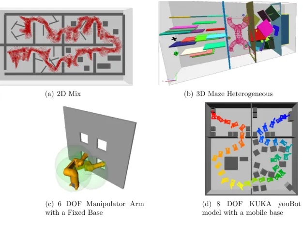
We look at a variety of input problems including 2D and 3D environments (see Figure 4.1) in industrial settings, narrow regions and highly heterogeneous environments.

• 2D-Heterogeneous, rod-like rigid robot. (Figure 4.1(a)) A long

rectan-gular rigid robot in a heterogeneous environment containing 8 different rooms of different types including cluttered, free, and blocked regions. The start is at the bottom left, and the goal is located at the top left. The robot must traverse each room to solve the query.

• 3D-Heterogeneous, spherical rigid robot. (Figure 4.1(b)) A spherical

robot must traverse 4 rooms separated by walls . These rooms include very narrow, cluttered, and maze regions. We allow roadmap construction to take 1200 seconds and provide 8 samples spread uniformly for querying. We then measure performance as the percentage of possible queries solvable from these samples by the roadmap.

• 6 DOF Manipulator arm. (Figure 4.1(c)) A 6 degree-of-freedom

manipu-lator arm with initial and final configurations inside a narrow passage where the robot has to pull out an object successfully from the bottom right window and place it in the bottom right window. This space between the robot and

(45)

the wall is made so narrow so that the robot would have to rotate 360 degree in the opposite direction to get to the other window.

• 8 DOF KukayouBot [60]. Figure 4.1(d) An 8 DOF robot in an environment

with four different rooms. Its base has 5 DOFs that allow it to move forward, backward and rotate, and its arm has 3 DOFs. The robot moves through different rooms with narrow passages and arrives at a destination where it performs an action (grasps or puts an object down).

The sampling methods that we compare to are Uniform sampling [58], OBPRM [8], Gauss [17], Bridge Test [46],UOBPRM [25], global learning for sampling (GLS), and our local learning applied to sampling (LLS). For connection methods, we use K-Closest, K-Closest,K-Rand, R-Closest,K-Rand, with k = 10 and k2 = 3k as de-termined in [79], and r as the average pairwise distance among a sample set of con-figurations. global learning for connection (GLC) and local learning for connection (LLC).

We use the StraightLine local planner and the RotateATS local planner [5] with s = 0.5. RotateATS attempts to find a path by translating from configuration qA to qB the portion of the distance denoted by s, rotating about its axis, and then translating the remaining way to qB.

4.2.1 Single Query Results

Here we show the performance in single query scenarios. Roadmaps are incrementally constructed until the query is solved. We measure performance as the time to solve the query and compare results using the various connection methods, global learning methods and local learning methods.

(46)

(a) 2D Mix (b) 3D Maze Heterogeneous

(c) 6 DOF Manipulator Arm with a Fixed Base

(d) 8 DOF KUKA youBot model with a mobile base

Figure 4.1: Environments studied.

4.2.1.1 Learning during Sampling

In this section we apply learning during the sampling phase only (LLS) and compare with individual methods and GLS.

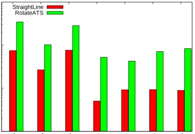
• 2D Mix Environment (Figure 4.1(a))

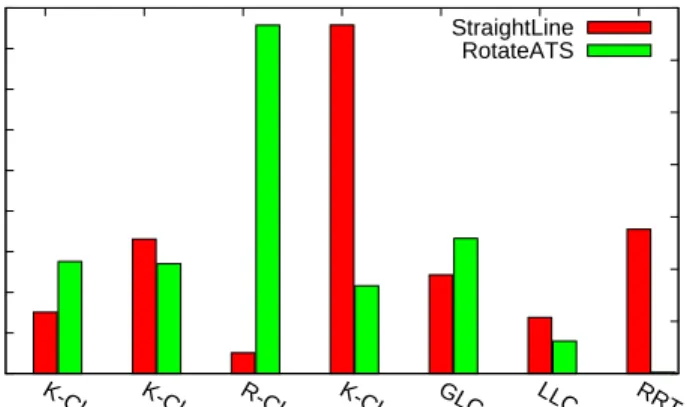
Figure 4.2 shows the time to solve the query for each sampling method studied in the context of StraightLine local planning (red bars and y axis on the left) and RotateATS local planning (green bars and y axis on the right). OBPRM performs best using the StraightLine local planner and Gaussian using the RotateATS local planner. Using GLS and LLS, we see that they perform

(47)

similarly and second best to the best performing methods for StraightLine and comparable for RotateATS with the best performing method.

1 10 100 1000

Uniform Bridge UniformOBPRMOBPRM Gauss GLS LLS

Time

StraightLine RotateATS

Figure 4.2: Query time for 2D Heterogeneous for Different Sampling Methods

• 6 DOF Manipulator Arm with a Fixed Base

We provide results for the time, collision call, number of nodes and number of edges produced and the edge to node ratio (in node degree).

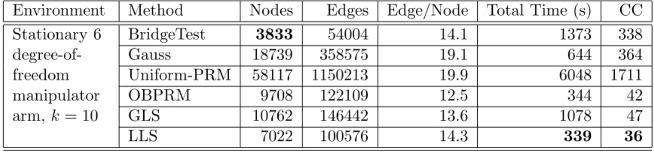
The results in Table 4.1 show that for individual methods, OBPRM uses the least amount of time while Bridge test uses the smallest number of nodes but the time taken to solve the query indicates that these nodes are expensive due to the time Bridge Test needed to solve the query. Results with GLS show some improvement in the time second to OBPRM. However, results using LLS show an improvement in performance both in regards to the time taken to solve the

(48)

query and a reduced number of connected components. LLS performs better than the best individual method.

Table 4.1: Each method constructs a roadmap until the query is solved. GLS and LLS is comprised of the other 4 sampling methods. All results are averaged over 10 runs. CC is number of connected components present. Boldface entries indicate the most desirable (e.g., shortest running time, Nodes, Edges etc.).

Environment Method Nodes Edges Edge/Node Total Time (s) CC Stationary 6 degree-of-freedom manipulator arm,k_{= 10} BridgeTest 3833 ₅₄₀₀₄ _14.1 ₁₃₇₃ ₃₃₈ Gauss 18739 358575 19.1 644 364 Uniform-PRM 58117 1150213 19.9 6048 1711 OBPRM 9708 122109 12.5 344 42 GLS 10762 146442 13.6 1078 47 LLS 7022 100576 14.3 339 36

• 8 DOF KUKA youBot model with a mobile base

We perform single query experiments and record the time needed to solve the query.

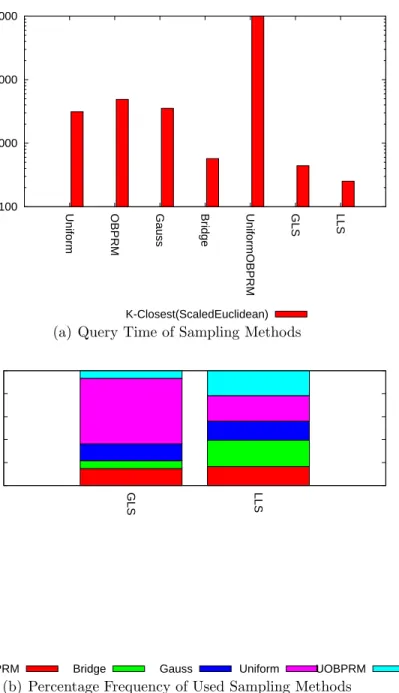
Figure 4.3(a) shows the time needed to solve the query in the KukayouBot environment using the different sampling methods listed. Here we determine how each of the sampling methods performs including evaluating both global and local learning during the sampling phase.

In Figure 4.3(a) we see that the LLS and GLS are better than all the in-dividual methods. LLS performs better than GLS in this experiment which indicates that learning is important during the sampling phase. The Bridge Test performs better in terms of time to solve the query than the other sampling methods where learning is not applied.

(49)

100 1000 10000 100000

Uniform OBPRM Gauss Bridge UniformOBPRM GLS LLS

Time

K-Closest(ScaledEuclidean) (a) Query Time of Sampling Methods

0 0.2 0.4 0.6 0.8 1 GLS LLS Time

OBPRM Bridge Gauss Uniform UOBPRM

(b) Percentage Frequency of Used Sampling Methods

Figure 4.3: Query time and Frequency of Usage for Different Sampling Methods

Figure 4.3(b) shows the frequency of usage of the different sampling methods in GLS and LLS. We see that GLS in most cases learns to use Uniform/Basic PRM sampling which is the simplest algorithm and thus would record a smaller cost

(50)

which GLS leverages on. However it does not learn the Bridge Test sampling method which from our results (see Figure 4.3(a)) is the better performing individual sampling method. LLS utilizes all the available sampling methods efficiently and it records the smallest time needed to solve the query.

4.2.1.2 Learning during Connection

In this section, we investigate the performance of the local learning method during the connection stage (LLC) and compare performance with individual methods.

• 2D Mix Environment

Figure 4.4 shows the time to solve the query for each method studied in the context of StraightLine local planning (red bars and y axis on the left) and Ro-tateATS local planning (green bars and y axis on the right). For StraightLine, R-Closest,K-Rand solves the query in the least time followed by LLC. LpSwept performs the worst because of its high computational cost. LpSwept is a more accurate method but due to the area covered during a sweep of the robot, such accuracy is not needed for StraightLine local planning. We also see that there is more time overhead needed to solve the query using RRT in comparison to both GLC and LLC. Note that LLC does better than GLC because the envi-ronment is heterogeneous, and there are no explicit subdivisions. Thus, local learning is needed.

With RotateAtS, we see a change in performance of the individual connection methods. Specifically, we see that LpSwept performs better here than before. ScaledEuclidean performs worse than LpSwept because it does not predict well the feasibility of RotateATS as it over-penalizes candidates with large rotation differences. LLC was able to take advantage of this change in performance

(51)

18 19 20 21 22 23 24 25 26 27

K-Closest(ScaledEuclidean)K-Closest,K-Rand(ScaledEuclidean)R-Closest,K-Rand(ScaledEuclidean)K-Closest(LpSwept)GLC LLC RRT 20

40 60 80 100 120 140 160

StraightLine Time(sec) RotateATS Time(sec)

Figure 4.4: Running time in the 2D Mix Heterogeneous environment using different local planners averaged over 10 runs.

and clearly outperforms all the other methods. Again, LLC outperforms GLC because of the issue of heterogeneity.

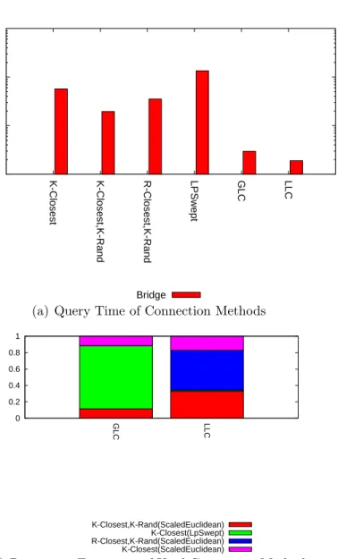
The results in Figure 4.3(a) help us select the sampling method (Bridge Test) to utilize for this experiment. Figure 4.5(a) shows time needed to solve the query using the Bridge Test as a sampling method and the different connection methods including GLC and LLC. We perform this experiment to determine if applying learning during the connection stage is beneficial.

From the plots, we see that LLC outperforms all the other methods. It outper-forms the other methods by a magnitude of 10 as is the case with the LpSwept method. This result indicates that learning is indeed important during the connection phase.

(52)

Figure 4.5(b) shows the performance frequency of usage of the connector meth-ods for learning employed during the connection stage. Here we see that GLS learns LpSwept which is not one of the better connection methods. GLC’s performance as earlier discussed in [35] is a result of the need to partition the environment to get good results which we did not do in these experiments. LLC however, utilizes the methods more which is an important feature of the local learning approach, i.e., their ability to utilize resources in a more intelligent way, which in this case is being able to use the methods available as the need arises.

4.2.1.3 Learning in Both Phases

Figure 4.6(a) shows the time needed to solve the query when learning (global and local) is applied to both the sampling and connection phase. Our results show that applying local learning during sampling and global learning to con-nection solves the query in the shortest time.

We see that applying local learning to sampling and global learning to connection is the best performing combination, followed closely by a global sampling and then local connection approach. Figure 4.6(b) shows the frequency of usage during learning both for sampling and connection and we see that the methods utilize all available methods in it’s list better than other methods.

GLS in most cases learns to use Uniform/Basic PRM sampling which is the simplest algorithm and thus would record a smaller cost which the global method would leverage on. However, global connection learning in most cases picks the LpSwept method which is a method that spans the volume of the space when identifying

(53)

10 100 1000 10000

K-Closest K-Closest,K-Rand R-Closest,K-Rand LPSwept GLC LLC

Time

Bridge

(a) Query Time of Connection Methods

0 0.2 0.4 0.6 0.8 1 GLC LLC Frequency K-Closest,K-Rand(ScaledEuclidean) K-Closest(LpSwept) R-Closest,K-Rand(ScaledEuclidean) K-Closest(ScaledEuclidean)

(b) Percentage Frequency of Used Connection Methods

Figure 4.5: Query time and Frequency of Usage for Different Connection Methods using Bridge Test Sampling Method

(54)

10 100

GLS-GLC LLS-GLC GLS-LLC LLS-LLC

Time

(a) Query Time with Learning Applied to both Sampling and Connection

0 0.2 0.4 0.6 0.8 1

GLS-GLC LLS-GLC GLS-LLC LLS-LLC Global-Global Local-Global Global-Local Local-Local

Time OBPRM Bridge Gauss Uniform UOBPRM K-Closest,K-Rand LpSwept R-Closest,K-Rand K-Closest

(b) Percentage Frequency of Usage during the Sampling and Connection Phase

Figure 4.6: Query Time and Frequency of Usage during both phases of PRM con-struction

(55)

4.2.2 Multi-Query Experiments

In this section, we show the performance of the various methods in multi-query sce-narios. Roadmaps are constructed within a fixed amount of time. We then count how many queries from a set of random samples are solvable by the resulting roadmap. We also look at the percentage of roadmap nodes contained in the largest connected component. This gives us indicators for coverage and connectivity. We perform multi-query experiment in the 3D Maze Environment and show behaviors of learn-ing in the sampllearn-ing and connection stages and when appied to both.

4.2.2.1 Learning in Sampling

Figure 4.7(a) shows that the sampling method using OBPRM solves more queries than the other methods. We see a higher percentage of nodes in its largest connected component as shown Figure 4.7(b) using the RotateAtS local planner and Straight-Line local planner when compared with the individual methods. Using the GLS, we see an improvement in performance for the StraightLine planner and a comparable method to OBPRM using the LLS the RotateAtS planner.

4.2.2.2 Learning in Connection

Figure 4.8(a) (bars in red), shows the percentage of queries solved and Figure 4.8(b) (bars in red) the percentage of nodes in the largest connected component for each method using the StraightLine local planner. LLC solves more queries than the other methods by almost a factor of 2. We see a comparably higher percentage of nodes in its largest connected component. LLC outperforms global connection learning due to the absence of explicit partitioning.

(56)

0.2 0.3 0.4 0.5 0.6 0.7 0.8 0.9

Uniform OBPRM Gauss Bridge UniformOBPRMGLS LLS

Query Solved

(a) Percentage of Queries Solved

0.25 0.3 0.35 0.4 0.45 0.5 0.55 0.6 0.65 0.7 0.75 0.8

Uniform OBPRM Gauss Bridge UniformOBPRMGLS LLS

Nodes

(b) Percentage of Nodes in the Largest Connected Component

Figure 4.7: Learning in Sampling for the 3D Maze Heterogeneous environment using different local planners averaged over 10 runs.

LLC is the second best in terms percentage of queries solved. Individual connection method performance has changed with the different local planners, but LLC still outperforms global connection learning.

(57)

15 20 25 30 35 40

K-Closest(ScaledEuclidean)K-Closest,K-Rand(ScaledEuclidean)R-Closest,K-Rand(ScaledEuclidean)K-Closest(LpSwept)GLC LLC

Query Solved

(a) Percentage of Queries Solved

30 35 40 45 50 55 60 65 70

losest(ScaledEuclidean)K-Closest,K-Rand(ScaledEuclidean)R-Closest,K-Rand(ScaledEuclidean)K-Closest(LpSwept)G