Unsupervised Anomaly Detection in Sensor Data used for Predictive Maintenance

Unsupervised Anomaly Detection in Sensor

Data used for Predictive Maintenance

MASTER THESIS

Author: Maria Erdmann

Faculty supervisor: Prof. Dr. Christian Heumann Department of Statistics

Faculty of Mathematics, Informatics and Statistics Ludwig–Maximilians–University München

External supervisor: Dr. Sebastian Kaiser Munich Re

Königinstrstraße 107 80802 München

III

Statutory Declaration

I declare that I have developed and written the enclosed Master’s Thesis completely by myself, and have not used sources or means without declaration in the text. Any thoughts from others or literal quotations are clearly marked. The Master’s Thesis was not used in the same or in a similar version to achieve an academic grading or is being published elsewhere.

Munich, December 03, 2018

... Maria Erdmann

IV

Abstract

With the emergence of “Industry 4.0” and advances in technology, anomaly detection on sensor data has become increasingly important within the area of predictive maintenance. This thesis deals with sensor data that are unlabeled, unevenly spaced time series, which makes anomaly detection a challenging task. It provides a literature overview on unsuper-vised anomaly detection methods suitable for unevenly spaced time series and introduces two new methods for anomaly detection, which are based on the Pattern Anomaly Value (PAV) algorithm proposed by Chen and Zhan (2008). The PAV algorithm is the only method explicitly described by their authors as being suitable for unsupervised anomaly detection on unevenly spaced time series. However, it has some limitations, which the new modifications aim to overcome. The PAV and its modifications are compared with four baseline methods from Statistical Process Control, which are adapted according to the present application. All methods are implemented in Python and are applied to the sen-sor data. Comparative analyses indicate low similarity between the results of the baseline methods and those of the PAV variants, which induced the idea to combine the results of all methods in an ensemble approach. An experiment on simulated data with manually added outliers enables performance evaluation and shows promising results for the ensemble.

CONTENTS V

Contents

2.2 Sliding Window Approaches . . . 15

2.3 Time Series Approaches . . . 17

2.4 Approaches For Streaming Data . . . 18

3 Data 22 3.1 Sensor Data . . . 22

3.1.1 Data Access and Preparation . . . 23

3.1.2 Descriptive Statistics . . . 25

3.2 Simulated Data . . . 29

4 Baseline Methods for Anomaly Detection 31 4.1 The 3σ-Rule . . . 31

4.2 The 3σ-Rule Based on a Rolling Average . . . 34

4.3 Exponentially Weighted Moving Average . . . 37

4.4 Percentile Method . . . 40

5 PAV: Anomaly Detection for Unevenly Spaced Time Series 41 6 Anomaly Detection with Modifications of PAV 44 6.1 Kernel Density Estimation . . . 45

6.2 Copulas . . . 49

7 Experimental Analysis and Results 54 7.1 Application to Simulated Data . . . 54

7.2 Application to Sensor Data . . . 64

7.3 Implementation and Application of the Copula PAV . . . 76

CONTENTS VI

References 95

A Appendix 102

A.1 Benchmark Experiment: Bandwidth Selection . . . 102

A.2 Simulated Data . . . 106

A.2.1 Performance Measures . . . 106

A.3 Sensor Data . . . 109

A.3.1 Additional Figures and Tables for all Channels . . . 109

A.3.2 Additional Figures and Tables for Temperature . . . 112

A.3.3 Additional Figures and Tables for Object Temperature . . . 113

A.3.4 Additional Figures and Tables for Humidity . . . 114

A.3.5 Additional Figures and Tables for Pressure . . . 116

A.3.6 Additional Figures and Tables for Magnetic Field x-Direction . . . 117

A.3.7 Additional Figures and Tables for Magnetic Field y-Direction . . . 119

A.3.8 Additional Figures and Tables for Magnetic Field z-Direction . . . . 120

1. INTRODUCTION 1

1

Introduction

Anomaly detection is the process of finding unusual patterns that deviate from their ex-pected behavior. The research field of anomaly detection is complex and broad with many fields of application. One application is predictive maintenance, the process of collecting and evaluating data from machines to predict machine failure and degradation of the pro-duction capacity. In particular, data from various sources, such as equipment sensors, are analyzed to identify unusual patterns and to predict these undesirable events.

This thesis aims to present suitable methods for anomaly detection that can be used on sensor data within the application of predictive maintenance. Such data was provided by MunichRE, the collaboration partner of this thesis. The data originates from about 500 sensor devices that were either attached directly to machines, machine parts or placed within the surrounding facilities such as machinery rooms. The sensor devices record environmental quantities like ambient temperature, object temperature, humidity, pressure and strength of the magnetic field. The resulting data can be briefly described as unlabeled, continuous, unevenly spaced time series. This data structure makes anomaly detection a challenging task.

The objectives of this thesis are to provide a literature review on anomaly detection tech-niques that are suitable for the specific data at hand and to implement those methods, that were identified to be appropriate, in Python. These methods include the Pattern Anomaly Value (PAV) algorithm byChen and Zhan (2008), which is the only unsupervised anomaly detection method explicitly described as being suitable for unevenly spaced time series. Based on the work ofChen and Zhan (2008) two new methods are presented, which mod-ify the PAV algorithm in a way that its limitations can be overcome. The methods are called Kernel PAV and Copula PAV.

The PAV algorithm and its modifications were compared to four baseline methods, namely a method based on Shewhart charts, which is called the 3σ-rule, a modification of the 3σ-rule using a rolling average, the exponentially weighted moving average (EWMA) and a method based on percentiles. Since anomaly detection methods within the context of predictive maintenance should be able to handle streaming data, the selected methods were implemented in a way that they could be used for streaming applications. Subsequently, they were applied to the sensor data and analyzed. In particular, the results of the different methods were compared against each other. The results induced the idea to construct an ensemble of anomaly detection methods. The performance of this ensemble and the

1.1 Predictive Maintenance 2

individual methods were assessed within a simulation study.

The outline of this thesis is as follows: Chapter 1 provides - in addition to this brief introduction - some background on the concepts of predictive maintenance (Chapter 1.1) and anomaly detection (Chapter 1.2) as well as the link between these two concepts. In Chapter 2, a literature overview on anomaly detection methods for temporal data is provided. Chapter 3 introduces the sensor data as well as the simulated data. Chapter 4 to 6 elaborate on the theory of the methods used in this thesis. These methods were applied to the sensor data as well as the simulated data and evaluated accordingly. The implementation and its results are reported in Chapter 7. Finally, Chapter 8 summarizes all findings, mentions various difficulties as well as drawbacks and gives an outlook.

1.1

Predictive Maintenance

Predictive maintenance is a maintenance strategy that monitors the actual operating con-dition of a machine, a system or plant equipment1, and uses this data to schedule all maintenance activities (Schreiner and J.,2018). Hence, this is a condition-based and data-driven approach to estimate when servicing of equipment is needed. To understand the nature of predictive maintenance, it is valuable to take a look at the main maintenance philosophies. These are: run-to-failure maintenance, preventive maintenance and predic-tive maintenance (Scheffer and Girdhar, 2004).

Run-to-failure maintenance, which is also called breakdown maintenance, is a reactive approach, where the equipment is serviced, i.e. it is repaired or replaced, when it breaks down. This approach is usually applied if the shutdown of the equipment for the service does not affect production and if material costs do not matter (Scheffer and Girdhar,2004). The disadvantage of run-to-failure maintenance is its high costs, which come from either high spare part inventory costs or costs due to a required fast delivery of spare parts from other vendors. Additionally, there are usually costs from overtime labor, high machine downtime and a low production availability (Mobley, 2002).

Applying preventive or time-based maintenance means to schedule all maintenance activi-ties at predetermined time intervals, which can be specific calendar days, run-time hours of a machine (Scheffer and Girdhar, 2004), or are based on mean-time-between-failure ( Mob-ley,2002). The goal is to repair or rebuild the equipment before a failure occurs. The main disadvantage of this approach is that the maintenance service may be applied too early or 1_{In the following, the term “equipment” will be used for all objects, where predictive maintenance can}

1.1 Predictive Maintenance 3

too late, which leads to reduced productivity (Scheffer and Girdhar, 2004). Additionally, scheduling is based on the experience of the maintenance manager (Mobley, 2002).

Predictive maintenance is often understood as condition-driven preventive maintenance approach (Mobley, 2002). However, others, such as Nagandhi et al.(2015) and Feldmann et al. (2017), see condition monitoring more as a philosophy on its own, which is the precursor and the basis of predictive maintenance. Condition monitoring checks the equip-ment’s actual mechanical condition, its efficiency and other indicators that determine the mean-time-to-failure or loss of efficiency (Mobley,2002). Common monitoring tools involve nondestructive tests like vibration monitoring, process parameter monitoring, thermogra-phy, tribology and visual inspection. Which diagnostic tool is suitable depends on the type of industry, the type of machinery and the availability of trained man power (Scheffer and Girdhar, 2004). Prognostic techniques are applied to the data from the monitoring pro-cess(es) in order to determine the mean-time-to-failure and other performance indicators (Lee et al., 2006). These are then used to schedule all maintenance activities.

The great advantage of this approach is that scheduling takes place in an orderly fashion, and that it saves costs, since spare parts can be ordered in a timely manner and do not need to be stocked. Additionally, it increases production capacity. However, an incorrect assessment of the deterioration process leads to potentially unnecessary maintenance ser-vices or serser-vices provided at the wrong time or not at all, which in turn leads to increased costs. Moreover, condition-based predictive maintenance requires specialized equipment, as well as trained and skilled personnel or, in case the maintenance service is outsourced, the willingness to pay for it (Scheffer and Girdhar, 2004).

In many cases, however, the concept of predictive maintenance is taken one step further. Thus,Feldmann et al. (2017) denote predictive maintenance as key innovation of Industry 4.0. In addition to the traditional diagnostic tools, this concept includes process perfor-mance data as well as data from sensors to assess the health of the equipment. It is about smart machines that are networked, and about automated methods to align the sys-tem’s operations and maintenance services. It involves an information flow infrastructure and automation in triggering the maintenance process, starting with ordering spare parts needed for repairing the equipment. Lee et al. (2014) terms this “e-maintenance” based on “intelligent prognostics” rather than predictive maintenance.

“Intelligent prognostics” is a systematic approach to continuously track the health or the degradation of a machine, and to extrapolate its temporal behavior in order to predict risks and unacceptable (anomalous) behavior, which is not only the failure of the equipment but

1.2 Anomaly Detection 4

also its loss of efficiency. This more holistic and systematic approach, which also can be found inScheffer and Girdhar(2004) andMobley(2002) in its basic ideas, aims to improve productivity, overall effectiveness, system safety, product quality and profitability. It is associated with a large amount of data that needs to be captured, stored and processed. In addition, it is advantageous to network the sensors and diagnostic processes. In many cases, the technical basis for advanced sensor technology is provided by the Internet of Things (IoT) (Schreiner and J., 2018).

1.2

Anomaly Detection

Anomaly detection, which is also denoted asoutlier detection, has neither a universally ac-cepted name nor definition. The reason for this heterogeneity is that research in this field comes from a wide variety of disciplines (Hodge and Austin, 2004). One of the commonly used definitions can be found in Chandola et al. (2009), who denote anomaly detection as the “problem of finding patterns in data that do not conform to the expected behav-ior”. These patterns are called outliers, outlying or discordant observations, anomalies,

abnormalities, deviants, exceptions, aberrations, surprises, peculiarities or contaminants

(Aggarwal, 2017; Hodge and Austin, 2004). In this thesis, the term outliers oranomalies, as well as outlier detection and anomaly detection will be used interchangeably. Outliers are observations that deviate so much from the other observations that one may assume that these observations originate from a different data-generating process than the remain-der of the data (Hawkins, 1980).

Anomaly detection is also sometimes called novelty detection or noise removal, although these terms are not the same. Novelty detection is more concerned about finding a pattern that has been hitherto unknown. Hence, novelty detection tries to find patterns in new observations that were not included in the training data. Noise removal, which is also calleddata cleansing(Goldstein and Uchida,2016), refers to the pre-processing step, where unfavorable observations are removed in order to get a signal, which can be used for analysis and inference (Choudhary, 2017).

In the recent applications of anomaly detection, the outlying observation itself is of partic-ular interest. Here, outliers are indicators of possible major adverse effects or deviations, whose detection is crucial for the application at hand (Suri et al., 2012). This is the understanding also this thesis focuses on.

Anomaly detection has many applications. In intrusion detection, the goal is to detect an unauthorized access in computer networks. Fraud detection plays a crucial role with

1.2 Anomaly Detection 5

respect to credit cards, but it is also a topic in health insurance. On the other hand, anomaly detection could be used by equity and commodity traders to monitor individual shares and markets in order to detect novel trends. Based on this, they identify buying and selling opportunities. In military, anomaly detection is used for the surveillance of enemy activities.

In connection with predictive maintenance, anomaly detection is critical. By monitoring complete manufacturing lines or single mechanical components such as motors or turbines and by applying anomaly detection techniques, a fault or considerable performance degra-dation can be detected early (Hodge and Austin, 2004). Chandola et al. (2009) call this

system health management orfault detection in mechanical units. They distinguish between

this application and the detection of defects in physical structures, such as cracks in beams or strains in airframes, which they refer to as structural defect detection. This distinction by Chandola et al. (2009) is made, because in system health management normal data for training is often readily available and used to model normality, while structural defect detection is about novelty or change point detection. There are many more applications than those already mentioned. A good overview is provided byHodge and Austin (2004). At first glance, implementing anomaly detection seems simple. By defining a representation of normal behavior of the data, it is straightforward to identify any observation that does not belong to this region. However, Chandola et al. (2009) names several factors that actually make outlier detection challenging: First, to define a region for normal behavior any notion of this normal behavior should be considered. This is difficult, since normal behavior very often keeps evolving. Secondly, the boundary between normal and anomalous behavior is very often continuous. In particular, observations close to the boundary cannot be unambiguously assigned to the normal or anomalous region. Additionally, the definition of an outlier is application-dependent, which often makes the methods used for anomaly detection not transferable or generalizable. Moreover, it is difficult to distinguish between anomalies and noise. Finally, one of the biggest challenges in anomaly detection is that labeled data is often not available or simply to expensive to acquire.

Hence, there is no straightforward approach for anomaly detection. On the contrary, most anomaly detection problems solve a specific problem formulation, which depends on the application at hand.

The anomaly detection problem consists of different aspects such as the nature of the data, the availability of labels, the type of anomaly that should be detected, and the desired output. Techniques to solve the specific problems originate from different areas such as

1.2 Anomaly Detection 6

4

·

Chandola, Banerjee and Kumar

which the anomalies need to be detected. Researchers have adopted concepts from

diverse disciplines such as

statistics

,

machine learning

,

data mining

,

information

theory

,

spectral theory

, and have applied them to specific problem formulations.

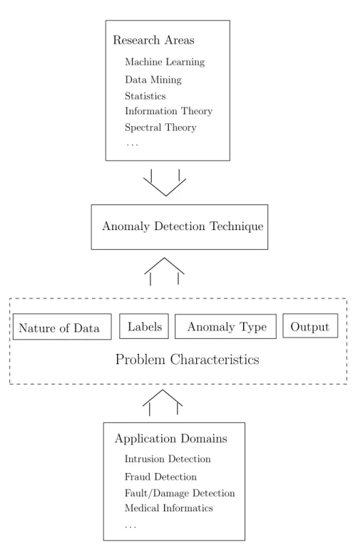
Figure 2 shows the above mentioned key components associated with any anomaly

detection technique.

Anomaly Detection Technique

Application Domains Medical Informatics Intrusion Detection . . . Fault/Damage Detection Fraud Detection Research Areas Information Theory Machine Learning Spectral Theory Statistics Data Mining . . .

Problem Characteristics

Labels Anomaly Type

Nature of Data Output

Fig. 2. Key components associated with an anomaly detection technique.

1.3 Related Work

Anomaly detection has been the topic of a number of surveys and review articles,

as well as books. Hodge and Austin [2004] provide an extensive survey of anomaly

detection techniques developed in machine learning and statistical domains. A

broad review of anomaly detection techniques for numeric as well as symbolic data

is presented by Agyemang et al. [2006]. An extensive review of novelty detection

techniques using neural networks and statistical approaches has been presented

in Markou and Singh [2003a] and Markou and Singh [2003b], respectively. Patcha

and Park [2007] and Snyder [2001] present a survey of anomaly detection techniques

Figure 1: Key components associated with anomaly detection. The application domain, e.g. damage detection, determines the characteristics of the problem, i.e. the nature of the data, whether labels are available, etc. These problem characteristics again deter-mine which anomaly detection methods, which can be from various areas such as machine learning, are suitable for the task. Reprinted from Chandola et al. (2009).

1.2 Anomaly Detection 7

statistics, machine learning, data mining, information theory, spectral theory and others. The interaction of the key components associated with anomaly detection are depicted in Figure1.

The four different aspects of anomaly detection are (Chandola et al., 2009):

Nature of Input Data Data can be either continuous, categorical or binary. Each data instance can be either univariate or multivariate, where in the latter case the data can be either of the same type (e.g. all data instances are continuous) or of different types. Data instances can be independent of or related to each other. If data instances are related, data are sequence data, spatial data or graph data. In sequence data, data instances are linearly ordered. Examples include genome sequences, protein sequences and time series data, the latter being of superior interest in this work. Time series data are characterized by their temporal continuity, which means that data is not changing abruptly, unless there are anomalous processes at work (Aggarwal, 2017).

Type of Anomaly Anomalies can be classified into three categories: point outliers, con-textual outliers and collective outliers (see Figure 2).

Point outlier If a single instance is anomalous with respect to the remainder of the

data, the observation is called a point outlier.

Contextual outlier If a data instance is anomalous in a specific context, it is termed

a contextual or conditional anomaly. In case of temporal data, these are in-stances that deviate remarkably from their adjacent values. Thus, these are point anomalies but with respect to their immediate neighborhood.

Collective outlier Collective outliers, which are also termedanomalous subsequences,

are a collection of data instances that behave anomalous with respect to the en-tire data set. Here, individual data instances may not be anomalous by them-selves, but the pattern, which they are part of, is anomalous.

While point outliers can occur in any type of data, contextual outliers can only be found in data where the instances are related to each other, for example, in temporal data. Furthermore, a point outlier or collective outliers can be transformed to contex-tual outliers, when analyzed with respect to its context. Aggarwal(2017) states that in time series data there are either contextual or collective outliers, whileGupta et al. (2014a) differentiates between point outliers and anomalous subsequences. Hence,

1.2 Anomaly Detection 8

one can assume that the terms point outliers and contextual outliers are sometimes used interchangeably in temporal data.

Data Labels When data labels are available, techniques operate in a supervised mode. Typically, anomaly detection is done by classification. This involves to train the model on labeled data, which is called training data, and to predict or identify the anomalies on some new data, called test data. In a semi-supervised setting, there are only labels available for the normal class. These labels, or in other words this normal data, are used for training, i.e. to establish a model of normality. This model is then used to identify anomalies in new data points (test data). If there are no labels available, techniques must operate in an unsupervised mode. In this case, no training data is needed. However, often unsupervised techniques can be implemented in a way that they suit the semi-supervised task. Thus, normal data can be used for training and prediction takes place on test data.

Output Anomalies can be either reported in the form of a score or as binary label (normal or anomalous). Most techniques output a score, which is a measure reflecting the degree of outlierness of a data instance. This score can be used to create a ranked list of anomalies. From this list, the user can select the top k anomalies or use a cut-off threshold to select the anomalies and to assign labels (normal or anomalous) to each data instance.

The four key factors, which are determined by the application, lead to a specific problem formulation. Given the data provided for this thesis and the application of predictive maintenance, also the problem of this thesis can be formulated with the presented four key characteristics. The sensor data can be describes as being continuous, unevenly spaced time series data, representing a strong temporal continuity. Although various environmental parameters are measured at the same time, the focus is on identifying outliers in univariate data streams. As there are no labels available, methods that can be used in an unsupervised mode are of primary interest. Additionally, in the application of predictive maintenance one is not interested in a specific type of outlier. All anomalies that indicate degradation or an effect of a major fault are of importance.

1.2 Anomaly Detection 9 2018-03-22 2018-03-29 2018-04-05 2018-04-12 2018-04-19 2018-04-26 2018-05-03 Time 20 25 30 35 40 45 Temperature [°C]

(a) Point outlier (red).

2009-01-01 2010-01-01 2011-01-01 2012-01-01 2013-01-01 Time 5 0 5 10 15 20 25 Temperature [°C]

(b) Contextual outlier (red).

2018-04 2018-05 2018-06 2018-07 2018-08 2018-09 Time 18 20 22 24 26 28 Temperature [°C]

(c) Collective outlier (red).

Figure 2: Types of anomalies. (a) and (c) are sensor temperature data provided for this thesis. (b) is the daily average temperature in Germany from 2009-2013 displaying an unusual temperature in April, 2012. Data was taken from Trading Economics (2018).

2. LITERATURE REVIEW 10

2

Literature Review

There has been extensive work on anomaly detection since the beginning of the 19th century (Chandola et al.,2009) and a large quantity of various methods has been developed in several research disciplines. Aggarwal (2017), Chandola et al. (2009) and Hodge and Austin (2004) provide comprehensive overviews on various anomaly detection methods. However, most of the work do not specifically consider the temporal aspect of the data. Research in anomaly detection for temporal data, especially time series data, is fragmented over different application domains, and a thorough understanding is missing. Particularly, insight is lacking, how the various methods are related to each other and differ from each other. An abstract classification of these anomaly detection methods based on their theoretical principles has not yet been provided. However, there is some work that tries to organize the multitude of methods.

Golmohammadi and Zaiane(2015) classify outlier detection into two orthogonal directions:

the transformation dimension and the dimension of the anomaly detection technique. The

transformation dimension refers to the way the data is preprocessed, i.e. transformed prior to applying a specific technique that aims to identify anomalies. The various types of transformations have different objectives:

Aggregation Aggregation reduces dimensionality by replacing a certain number of suc-cessive values with a representative value (e.g. average) of them. This refers to applying a low-pass filter, which suppresses the high frequency signals in order to reveal the low-frequency features.

Discretization Discretizising a time series means to convert the continuous data into cat-egorical data. For example, continuous values are mapped to letters of an alphabet. One such approach was proposed by Lin et al. (2007). The objective for discretiza-tion is reducing computadiscretiza-tional complexity, as it is, for example, used in Keogh et al. (2005)s’ HOTSAX algorithm.

Signal Processing With the help of, for example, Fourier transforms or wavelet trans-forms, data is mapped to a different space. This helps to detect anomalies at a different scale and may reduce dimensionality.

Differencing Differencing is used to stabilize the mean, hence, to make non-stationary time series stationary. For example, computing the change between consecutive ob-servations (1st-order differencing) helps to eliminate or reduce trend and seasonality

2. LITERATURE REVIEW 11

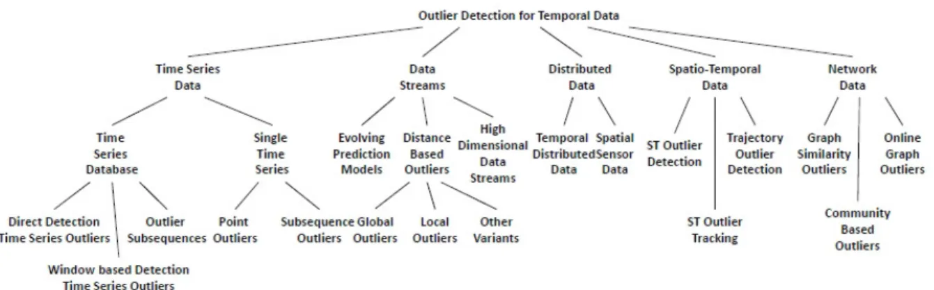
Figure 3: Overview on outlier detection in temporal data based on the various types of data. Reprinted from Gupta et al. (2014a,b).

in time series. Besides 1st-order differencing, it is occasionally necessary to compute 2nd-order differences to consider “the change in the changes”, or to do some sort of seasonal differencing (Hyndman and Athanasopoulos, 2018).

There are some disadvantages associated with transformation of the data. Firstly, the results of anomaly detection on the aggregated time series needs to be mapped back to the original time series in order to provide meaningful information. Discretization does not reduce dimensionality. Additionally, most discretization techniques require the whole time series in order to provide a meaningful alphabet, and thus, cannot be applied in a streaming setting. Moreover, distance measures may no longer be reasonable when data has been discretized or processed.

However, transformations provide the possibility to investigate different aspects of the data. Thus, combining transformation with anomaly detection methods results in a great variety of anomaly detection approaches.

Regarding the dimension of anomaly techniques, there are a couple of suggestions for categorizing or organizing the plentitude of methods. For example, Gupta et al.(2014a,b) provide an overview on outlier detection for temporal data, where methods are classified with respect to the actual type of data (see Figure 3). Thus, they distinguish between methods for time series data, data streams, distributed data, spatio-temporal data or network data. Furthermore, anomaly detection in time series data can be partitioned into anomaly detection on time series databases or in a single time series. For the latter, they claim that there are two types of anomalies: point anomalies and subsequences as outliers, which refer to anomalous shapes in the time series and are also called collective outliers.

2. LITERATURE REVIEW 12

Aggarwal(2017), as well, organizes the methods for outlier detection in time series by clas-sifying them according to the type of anomaly they detect. There, methods for contextual outliers are distinguished from methods for collective outliers.

A reasonable taxonomy of outlier detection methods that should be highlighted was pro-posed byBen-Gal(2005) and adopted bySuri et al.(2011), although it is not specifically for temporal data. Ben-Gal (2005) distinguishes between univariate and multivariate meth-ods, and betweenparametricandnon-parametricmethods. Parametric methods, which are also calledstatistical methods, assume that there is a known underlying distribution of the data. This distribution can be characterized by the probability density function f(x; Θ), whose model parameters Θ – if there are any – are estimated from the data (Eskin et al., 2001, quoted from Chandola et al., 2009). Using statistical methods, one assumes that normal data is generated by a specific stochastic model, while anomalous data do not orig-inate from this model. This means, that normal data is presumed to occur in regions of high probability of the stochastic model, while anomalous data tend to appear in regions of low probability. Hence, data instances that have a low probability are declared outliers. For the non-parametric techniques, no assumptions on the underlying distribution are made. The model structure is defined solely by the data (Chandola et al., 2009). The non-parametric techniques are further classified into distance-based, density-based and

clustering-based methods (Suri et al., 2011). The latter classification appears to be

some-how artificial, as there are great overlaps between the individual classes. Hence, for the purpose of this work, it is sufficient to distinguish between parametric and non-parametric methods.

All structural organizations provided by the surveys mentioned above seem reasonable. However, there are several reasons why it is not possible to simply use one of these organi-zations to provide a comprehensive overview on unsupervised anomaly detection methods for unevenly spaced time series. Firstly, since the sensor data used in this work is not la-beled, only methods for unsupervised anomaly detection will be reviewed. Secondly, many unsupervised methods presented by Aggarwal (2017), Chandola et al. (2009) and Gupta et al.(2014a,b) assume that normal training data is readily available. If this would be the case a model of normality can be fitted to the data, and anomaly detection takes place on some test data. However, in the case of this work, there is no a priori knowledge on whether the data is normal or not. Hence, also training needs to be done in an unsuper-vised manner. Additionally, the peculiarity of the sensor data is an unevenly spaced time

2.1 General Approaches 13

Anomaly Detection Methods

General Approaches Sliding Window Approaches Time Series Approaches

Evenly spaced time series

Unevenly spaced time series Figure 4: Structure of the literature overview provided in this work

series data, which considerably narrows down the methods that are applicable. Lastly, the methods presented should suit the predictive maintenance context or should actually be created for this specific application. Hence, this work tries to provide a distinctive orga-nization of methods for completely unsupervised anomaly detection on time series data for the application of predictive maintenance, based on the surveys mentioned so far. The structure is schematically presented in Figure 4.

Three types of anomaly detection techniques are distinguished: The first type does not consider the temporal aspect of the time series data and comprises approaches for anomaly detection for i.i.d. data. Hence, these are general approaches. They can be modified by using a sliding window, with the result that the temporal aspect of the data is now considered. The third type of methods, considers the time series structure specifically. Methods for evenly and unevenly spaced time series will be presented.

To round off this literature overview, a variety of anomaly detection methods for a stream-ing environment is presented, as streamstream-ing is of particular interest in predictive mainte-nance.

2.1

General Approaches

Although there is certainly a main drawback in applying techniques that do not consider the temporal correlation of adjacent data points, these methods are widely used in practice. With regards to the parametric techniques for anomaly detection, it is very common to assume that the data is normally distributed. Methods that are based on this assumption are Shewhart charts, the box plot rule and a couple of statistical tests.

Shewhart charts have their roots in Statistical Process Control (SPC). The Shewhart

method declares data instances as outliers, if they are more than 3σ (three times the standard deviation) away from the mean µ. Assuming a normal distribution, the µ±3σ

2.1 General Approaches 14

region contains 99.7% of the data instances (Shewhart,1931, quoted from Chandola et al., 2009). More details on this method are provided in Chapter 4.1.

The box plot rule (Laurikkala et al., 2000; Horn et al., 2001; Solberg and Lahti, 2005;

Guttormsson et al., 1999, quoted from Chandola et al., 2009) is a graphical approach to identify outliers. The boxplot is a 5-point plot displaying the median, the lower and upper quartile (Q1, Q3), as well as the largest non-outlying observations. Data points are declared outliers, if they are 1.5·IQR lower than Q1 or 1.5·IQR higher than Q3, where

IQR is the interquartile range (Q3−Q1). The 1.5·IQR rule is a heuristic proposed by Laurikkala et al. (2000) that makes the box plot rule equal to the Shewhart method with its 3σ-limits.

The Grubb’s test, also called maximum normed residual test, uses the z-score

z = |x−x|

s (1)

as statistic, where x is the mean and s the standard deviation of the sample. A data instance is declared an outlier, if

z > n√−1 n v u u t t2 α/(2n),n−2 n−2−t2 α/(2n),n−2 (2)

wheren is the size of the sample and t2

α/(2n),n−2 is theα/(2n) quantile of thet-distribution

withn−2 degrees of freedom. Thus, the hypothesis of no outliers is rejected at a significance level of α.

Other statistical tests are the student’s t-test (Surace et al., 1997; Surace and Worden, 1998, quoted from Chandola et al., 2009), the Rosner test (Rosner, 1983, quoted from Chandola et al., 2009) and the Dixon test (Hawkins, 1980, quoted from Chandola et al., 2009).

The disadvantage of these parametric methods is that they rely on the assumption that the data was generated from a specific distribution (here: Gaussian distribution). However, this assumption does not hold true in most cases (Chandola et al., 2009). In particular, these methods cannot detect outliers in small samples. Moreover, the mean, as a measure of central tendency, and the standard deviation, as a measure of scale, are heavily impacted by outliers. Hence, the indicator that guides anomaly detection, is itself altered by the presence of outliers. Thus, using non-parametric approaches for anomaly detection, such as using the median and the mean absolute deviation (MAD) instead of the mean and the

2.2 Sliding Window Approaches 15

standard deviation, is more robust (Rousseeuw and Croux, 1993). The MAD is defined as

M AD=c·median(|xi−median(x)|), i= 1, . . . , n,where median(x) is the median of the sample x = (x1, . . . , xn) and c is a constant determined by c= 1/Q3. If data is normally distributed, c= 1.4826. For anomaly detection, a common choice for the threshold is:

|xi−median(x)|

M AD >| ±3|, i= 1, . . . , n (3)

(Leys et al.,2013).

2.2

Sliding Window Approaches

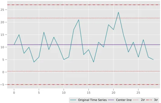
The problem with methods that do not consider the temporal dependency of the data is that they disregard possible seasonality, trends or change points in the data. Computing the standard deviation of a long time series may result in a large value (see Figure10) such that only global outliers can be detected. If the goal is to detect outliers that are anomalous with respect to their neighboring values, it is necessary to consider this neighborhood, i.e. to divide the time series into subsequences of a fixed window length m. By using a sliding

or rolling window, all possible subsequences are considered. Methods that use a sliding

window can be applied to evenly and unevenly spaced time series.

Hence, Shewhart’s 3σ-rule can be modified using a rolling mean, as it is described in more detail in Chapter 4.2.

An approach to use the median on time series data has been proposed by Basu and Meckesheimer (2007). They propose a two-sided and a one-sided median method, which they apply to sensor data.

For the two-sided median method, the medianmt=median(xt−κ, . . . , xt, . . . , xt+κ) of the values in a window of size 2κis computed. The window starts at time pointt−κand ends at t+κ. By using the absolute value of the difference between mt and xt and comparing this difference to a threshold, outliers are identified. In case |xt−mt| ≥τ,xt is labeled an outlier.

The one-sided median method is applied to identify outliers, when solely historic data is available. Here a one-sided median of the raw data x and a one sided median of the first differencesz =xt−xt−1 are computed:

˜

m(_tx) =median(xt−2κ, . . . , xt−1) (4)

˜

2.2 Sliding Window Approaches 16

Then, the predicted value for xt is computed as a weighted average:

ˆ xt= ˜m (x) t +κ·m˜ (z) t (6)

If |xt −x˜t| ≥ τ˜, the value xt is denoted an outlier. Although these methods provided good results, they are sensitive to the appropriate choice of thresholdτ and ˜τ, respectively, which needs to be determined by the user and therefore requires some knowledge on the application.

Hill and Minsker (2010) propose three anomaly detection methods that use a moving window. Particularly, a moving window of the lastm measurements

Dt=xt−m+1, . . . , xt (7)

is used to predict the next measurement xt+1 and to classify this measurement as

nor-mal or anonor-malous. Hence, their approach uses a one-step-ahead prediction model that takes Dt as input to predict xt+1. Then a prediction interval is computed and used to

determine whether xt+1 is an anomaly. The first method they propose for the one

step-ahead-prediction is the nearest cluster (NC) predictor. Similar training data are grouped to clusters based on their moving windows and the Euclidean distance metric is computed betweenxt+1 and each training sample2. The predicted value ofxt+1is calculated based on

the average of all measurements in the cluster that xt+1 maps to. The two other methods

for the one-step-ahead prediction are the single-layer linear network (LN) predictor and

the multilayer perceptron (MLP) predictor. The LN predicts xt+1 as a linear combination

of m previous measurements: ˆ xt+1 =b m−1 X i=0 wixt−i (8)

where b and {wo, . . . , wm−2} are the weights that are learned by the delta learning rule.

The MLP is a feed-forward network with sigmoid activation functions in the hidden layer and a linear activation function in the output layer. It is trained with the backpropagation algorithm based on gradient descent and momentum. The number of hidden layers, and nodes in the hidden layers, as well as the learning rate, the momentum and the number of epochs are hyperparameters that were selected by a trial-and-error approach. The approach 2_{In this work, a training sample consists of a input vector, which is the moving window D}t _{and an}

2.3 Time Series Approaches 17

by Hill and Minsker (2010) has the great advantage that the threshold for differentiating between normal and anomalous data is not user-defined, but rather a prediction interval that is based on an estimate of the standard deviation, for which 10fold cross-validation is used. Additionally, it is fast and scalable to large data sets.

One additional algorithm should be mentioned here, although this method is intended to be applied on evenly spaced time series and no work has provided evidence yet that this method works well on unevenly spaced time series. However, investigation of the methodology used suggests that modification of the algorithm is possible, such that it can be used for unevenly spaced time series. Wei et al. (2005) use a lead and lag sliding window, and within each window, the time series is discretized via Symbolic Aggregate Approximation (SAX) (Lin et al.,2007). A modification of SAX to unevenly spaced time series data may be achieved by applying time horizons instead of specifying the number of observations in the aggregation step. The SAX representation is then used to create so called chaos game bitmaps, which are matrices representing the count of single letters or subwords occurring in the SAX representation of the time window. Subsequently, the distance between the bitmaps is measured and reported as anomaly score at each time instance.

2.3

Time Series Approaches

Time series approaches are techniques that consider the internal structure of the time series data. This means, that they consider that data may have a trend or seasonal variation and that observations close together are correlated (autocorrelation). But these approaches can solely be applied to evenly spaced time series. Additionally, these methods often require that normal training data is available. So far, little work has been published on unsupervised anomaly detection for unevenly spaced time series. Namely, there is a single work by Chen and Zhan (2008), which claims to be applicable to unevenly spaced time series. Chen and Zhan(2008) propose an approach where infrequent patterns within a time series are indicative for anomalous patterns. More details on this method are provided in Chapter 5.

Traditionally, unevenly spaced time series were transformed to evenly spaced time series by use of some form of interpolation. Then the common time series methods can be applied to the transformed data. Since this is still an approach commonly used in practice, some methods for anomaly detection on evenly spaced time series are shortly presented.

2.4 Approaches For Streaming Data 18

is also often referred to as prediction-based orregression model based outlier detection. It consists of two steps: First, a regression model is fitted to the data, such as an autoregres-sive (AR), moving average (MA), autoregressautoregres-sive moving average (ARMA) or integrated autoregressive moving average (ARIMA) model. Second, the anomaly score is computed based on the residual of the test instance. Hence, the difference between the predicted and the observed value of the test instance is computed. The magnitude of this difference serves as anomaly score. As the presence of anomalies during training might influence the result of the model, and may lead to inaccurate results in the worst case, using robust regression is advisable (Rousseeuw and Leroy, 1987, quoted from Chandola et al., 2009). For example, in Bianco et al. (2001, quoted fromChandola et al.,2009) and Chang et al. (1988, quoted from Aggarwal, 2017) robust anomaly detection on ARIMA models are ap-plied. The robustness originates in a robust parameter estimation and robust filtering. Chen and Liu (1993) jointly estimate model parameters and outlier effects by successively analyzing the data with adjusted ARMA models and by removing potential outliers that were detected in a previous step.

For detecting collective outliers (anomalous subsequences) within a time series, discord discovery by Keogh et al. (2005) is a common method. A time series discord is defined as being maximally different to the remaining time series subsequences. In their paper, they propose two types of algorithms. The first approach is brute force, since the discord search, i.e. the search for the subsequence that has the largest distance to its nearest non-self match, is done by computing the Euclidean distances between each pair of sub-sequence. The second approach is HOTSAX, which improves computational efficiency by using a data structure that is based on SAX.

2.4

Approaches For Streaming Data

In this chapter, some methods for anomaly detection in streaming data are introduced, since ultimately anomaly detection in the application of predictive maintenance aims to forecast future trends and to detect anomalies at an early stage in a streaming context. Streaming data adds additional challenges to the demanding task of unsupervised anomaly detection. Firstly, data must be processed in real-time. Batch processing and a look into the future is not possible. Secondly, often there is a multitude of streams providing information on the application under investigation. Thirdly, anomaly detection should be performed in an unsupervised and automated fashion, where the latter means that the

2.4 Approaches For Streaming Data 19

hyperparameters of the methods should not be adjusted manually. Moreover, anomalies should be detected as early as possible and, at the same time, the false positive rate as well as the false negative rate, should be kept small. In addition, every application has its own constraints.

The following methods are consolidated by the Numenta Anomaly Benchmark (NAB) project, which is an open source framework that provides a “controlled and repeatable environment of [...] tools to test and measure anomaly detection algorithms on streaming data” (Lavin and Ahmad, 2015). They provide data from different application domains that are partially labeled and a scoring system. Both can be used to evaluate perfor-mance of anomaly detection algorithms for streaming data. The project is designed to help researchers to evaluate their own methods and to compare them with existing meth-ods for streaming data. The methmeth-ods implemented includeHierarchical Temporal Memory

(HTM), Skyline developed by Etsy.com, Twitter’s anomaly detection methods, Bayesian

Online Changepoint detection,EXPoSE andMultinomial Relative Entropy (Ahmad et al.,

2017).

HTM is a theory inspired by neuroscience, especially by the structure and functionality of the neocortex of the mammalian brain. In the context of anomaly detection, HTM is used to make multiple predictions for an instreaming observationxt+1. At time t+ 1 these

predictions are compared to the observed value and an anomaly score is calculated. The anomaly detection system retains information on the distribution of the anomaly scores computed so far. Therefore, at every time step a likelihood, on whether the current anomaly score is from the respective distribution, can be calculated. The anomaly likelihood serves as a threshold to finally identify whether the instreaming data point is an anomaly (Lavin and Ahmad, 2015).

Skyline is a real-time anomaly detection system based on an ensemble of (simple) detectors and a voting scheme. A data instance is flagged as being anomalous if the majority of the detectors agree that this data instance is an anomaly. A couple of simple detectors are built-in, such as the deviation from moving average (this refers to the Shewhart method using a rolling average explained in2.2), the deviation from the least square estimate and the deviation from the histogram of passed values (Lavin and Ahmad, 2015; Stanway, 2013).

Twitter provides two algorithms that make use of the combination of various statistical techniques. Namely, these are Seasonal-ESD (S-ESD) and Seasonal-Hybrid-ESD (S-H-ESD). In S-ESD, the time series data is decomposed to eliminate trend and seasonality.

2.4 Approaches For Streaming Data 20

Then ESD (Extreme Studentized Deviant) (Rosner,1983) is applied to the residual compo-nent of the time series. ESD, also called Rosner’s test, is a further development of Grubb’s test. While Grubb’s test only detects single outliers in a univariate data set, which follows an approximately normal distribution (NIST/SEMATECH, 2013b), the ESD can detect multiple outliers and requires only an upper boundk for the suspected number of outliers. Depending on this upper bound, k tests are performed, with the following hypothesis:

H0: There are no outliers in the data set.

H1: There arek outliers in the data set.

The test statistic is computed for the k most extreme values in the data set:

Rk=

maxk|xk−x|

s (9)

where x and s denotes the sample mean and the sample standard deviation, respectively. The most extreme values are those that maximize |xk−x|. The statistic is compared to a critical value λk, and the data instance is removed from the data set, if it is flagged an anomaly. Then the critical value λk is recalculated. This process is repeated k times (Hochenbaum et al., 2017; NIST/SEMATECH, 2013b).

S-ESD is suitable for detecting local and global outliers, but it suffers from the problem that mean and standard deviation – as explained earlier – are highly sensitive to outliers. This results in a high rate of false negatives. To solve this problem, S-H-ESD was introduced, which uses robust statistics such as the median and the MAD (Hochenbaum et al., 2017).

Bayesian Changepoint detection proposed by Prescott Adams and MacKay (2007) is a

Bayesian algorithm, that identifies online, whether there is a state transition in a sequence of data. It uses the Bayes’ theorem to calculate the posterior probability of the current run lengthri, which refers to the time that has elapsed since the last change point. Given the run length at time t, the run length at time t+ 1 is either be set back to zero (if a change point is detected) or increased by 1 (if current state continuous).

EXPoSE (EXpected Similarity Estimation) by Schneider et al. (2016) is a kernel-based

estimator that computes the similarity between a new data point and the distribution of regular data seen so far. A score, which is the likelihood for belonging to the normal class, is computed as the inner product between the feature map φ(z) and the kernel mean map

µ[_P] of the distribution of the normal data_P:

2.4 Approaches For Streaming Data 21

The estimator can be learned incrementally and is therefore suitable for the streaming application.

Wang et al. (2011) introduced the Multinomial Relative Entropy, which uses the relative entropy statistic to test multiple hypotheses. Each observed value is compared against mul-tiple null hypotheses. If the new data instance does not agree with one of the hypotheses it is declared anomalous and a new hypothesis is declared. For rejecting or accepting the hy-pothesis, the relative entropy statistic is computed. Its value is compared with a threshold that represents an acceptable level of false negatives of the Chi-square distribution.

3. DATA 22

3

Data

This chapter introduces the data basis for the present work. The sensor data provided by MunichRe are introduced in Chapter 3.1, along with some summary statistics. As these data are not labeled, performance evaluation, as is commonly used in supervised learning, is not possible. In order to assess performance of the methods presented in this thesis, data was simulated. These data are presented in Chapter 3.2.

3.1

Sensor Data

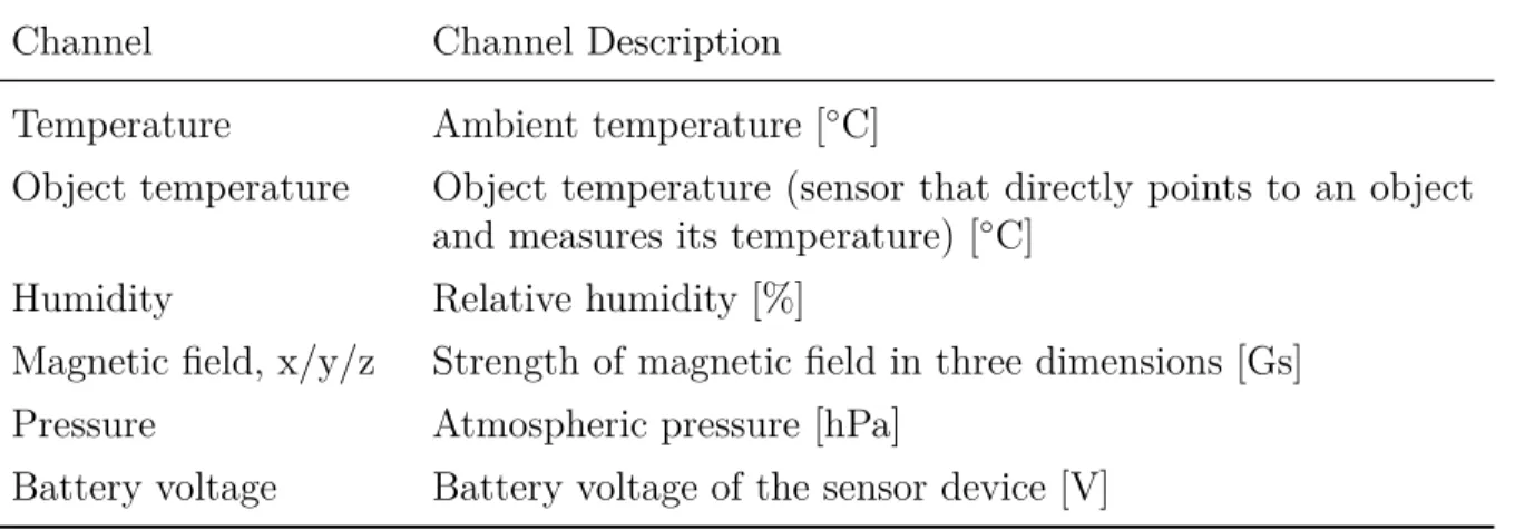
The data base for this work was provided by the IoT Department of MunichRe. It com-prises sensor data from machinery, technical equipment and surrounding facilities, such as machinery rooms. In 2017, several battery-powered sensor devices were installed in various places of 17 small and medium sized enterprises (SMEs), manly from manufacturing in-dustry. Popular locations were electrical cabinets, server rooms or cooling compressors. A sensor device can measure multiple quantities. These quantities, which are called channels, are listed and described in Table 1

Table 1: Channels of the sensor devices. The unit of measurement is depicted in square brackets.

Channel Channel Description

Temperature Ambient temperature [◦C]

Object temperature Object temperature (sensor that directly points to an object and measures its temperature) [◦C]

Humidity Relative humidity [%]

Magnetic field, x/y/z Strength of magnetic field in three dimensions [Gs] Pressure Atmospheric pressure [hPa]

Battery voltage Battery voltage of the sensor device [V]

Depending on the application, i.e. whether the sensor is attached to a compressor, or placed within an electrical cabinet or is aimed to measure the room’s temperature, certain channels record data, while others are switched off, because they are not relevant to the application.

3.1 Sensor Data 23

Overall, there were 567 sensor devices installed, each of them having a unique identifier (uid).

Recording of the data started in February, 2018 for some data sets, while for others the start was a little later.

The sensor device took measurements on a very high frequency, however a signal to the platform was sent on a less frequent basis to safe battery of the sensor device. But if changes in measurements between the regular transmission times were above or below a certain threshold, then the affected measurement was sent to the platform immediately. The rules for measuring and sending were defined and implemented for each channel individually, but are not available for this work.

The result of the data generating process is that data are represented as time series. Formally, a time series is defined as a series of data points indexed with time stamps:

X =hv1 = (x1, t1), v2 = (x2, t2), . . . , vn= (xn, tn)i, (11) where vi = (xi, ti) refers to a data point xi at time stamp ti.

In particular, the sensor data is characterized by varying sampling intervals ∆t =ti−ti−1

between successive time points. Time series with varying sampling frequencies, i.e. ∆t 6=

const, are called unevenly spaced time series. Since the sensor data are unlabeled, they

were not split into training set Xtrain and test set Xtest for analysis, rather the complete time series was used for training and predictions, hence X =Xtrain =Xtest applies.

3.1.1 Data Access and Preparation

Data was accessed per channel from a platform. For each channel, data were stored under the uid of the sensor device from which the data originated.

Not all sensor devices sent information to the platform and not all sensor devices could be accessed while dumping the data. Therefore, the total number of data sets per channel varies. Table 2 shows the resulting total number of data sets for each channel. Data sets that contained either no or just one observations were removed from the data base for analysis. In addition, some data sets dropped out, due to errors encountered during analyses. The number of data sets with one or no observation and the final number of data sets for analysis are shown in column 3 and 4, respectively of Table 2.

Channel battery voltage, which indicates the battery status of the sensor device, was not used for any analysis.

3.1 Sensor Data 24

Table 2: Number of data sets per channel.

Channel Noverall Nremoved Naf ter f iltering

Temperature 544 48 495 Object temperature 547 350 193 Humidity 547 50 496 Pressure 547 51 493 Magnetic field, x 529 286 259 Magnetic field, y 528 286 259 Magnetic field, z 529 286 260 Battery voltage 490 0 490

Due to a firmware update on the data platform, which lead to invalid measurements, specific data points needed to be erased. In particular, ambient and object temperature data greater than 150 degrees, a humidity greater than 100 percent and a pressure of greater than 1500 hPa were considered to be indicative of the firmware update. The af-fected period and all data points 2 hours before and 2 hours after the period were removed.

Since the anomaly detection methods implemented within the course of this thesis should not only be applied to the “raw” data, but also “transformed data”, data was transformed by using first-, second- and third-order differences of the raw data.

Differencing of time series is commonly used to make non-stationary time-series stationary. First-order differencing is defined by

∆xt=xt−xt−1 (12)

(Cowpertwait and Metcalfe, 2009). Hence, this is the change between each observation in the original time series (the raw data). Writing this with the backward shift operator B, results in ∆xt= (1−B)xt. Higher ordering differencing can be expressed with

∆n= (1−B)n (13)

3.1 Sensor Data 25

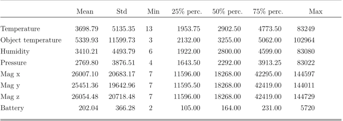
Table 3: Summary statistics describing the data sets’ length per channel.

Mean Std Min 25% perc. 50% perc. 75% perc. Max Temperature 3698.79 5135.35 13 1953.75 2902.50 4773.50 83249 Object temperature 5339.93 11599.73 3 2132.00 3255.00 5062.00 102964 Humidity 3410.21 4493.79 6 1922.00 2800.00 4599.00 83080 Pressure 2769.80 3876.51 4 1643.50 2292.00 3913.25 83022 Mag x 26007.10 20683.17 7 11596.00 18268.00 42295.00 144597 Mag y 25451.36 19642.96 7 11595.50 18268.00 42419.00 144011 Mag z 26054.48 20718.48 7 11596.00 18268.00 42419.00 144729 Battery 202.04 366.28 2 105.00 164.00 231.00 5720

std: standard deviation, min: minimum, perc: percentile, max: maximum

3.1.2 Descriptive Statistics

The average number of observations in the individual data sets varies with respect to the channel (see Table 3). While the average number of observations is between 25 451 and 26 054 for the sensors capturing the strength of the magnetic field, the average number of observations for the other channels ranges between 2770 and 5340. On contrary, the data sets for battery voltage has on average 202 observations. From the second column, it can be derived that the number of observations per data set varies quite a bit. The maximum number of observations observed in the data is 144 729 (for strength of magnetic field in the z direction).

Table 4presents summary statistics on the sampling frequencies of all data for each chan-nel. Sampling frequencies vary between 1 and maximum 16 764 342 seconds (= 194 days). Large sampling frequencies originate from data sets, where measurements needed to be removed within the course of data pre-processing. The median value shows that for most channels the regular sampling frequency was one hour (= 3600 seconds) or 300 seconds.

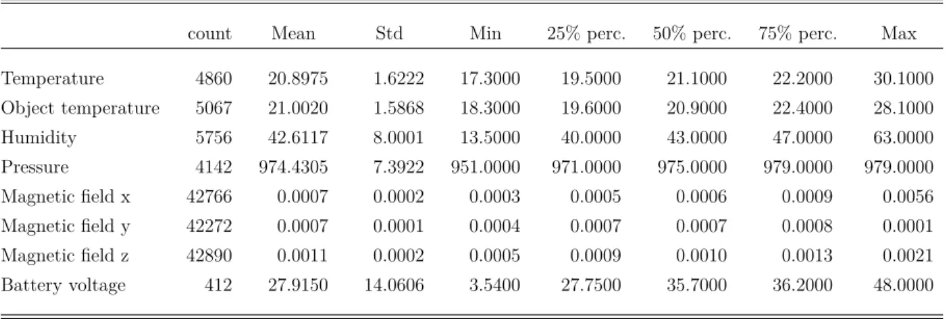
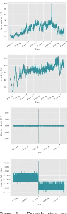
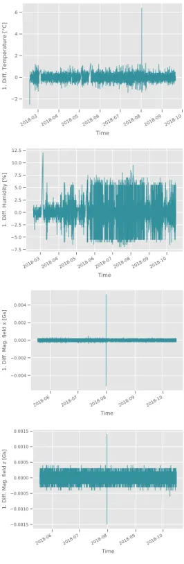
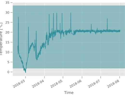
Each individual time series was plotted and summary statistics were computed. All plots and summary statistics can be found in the electronic appendix. As an example, the results of one sensor device, where all channels of the sensor device recorded data, are plotted in Figure5. The corresponding summary statistics are provided in Table5. Additionally, the first-order differences of the example are shown in Figure 6.

3.1 Sensor Data 26

Table 4: Summary statistics for sampling frequencies (in seconds) per channel.

Mean Std Min % perc. 50% perc. 75% perc. Max

Temperature 3466.44 56520.40 1 1200 3600 3600 16764342 Object temperature 2397.84 4493.79 1 118 1620 4599 12397776 Humidity 3994.96 54499.42 1 3600 3600 3601 12414106 Pressure 4822.94 80349.83 1 3600 3600 3658 15703482 Magnetic field x 314.30 11150.63 1 300 300 300 12234182 Magnetic field y 317.31 11209.19 1 300 300 300 12234182 Magnetic field z 314.15 11141.86 1 300 300 300 12234182 Battery voltage 68548.08 193052.22 1 1800 85904 86400 12485576

std: standard deviation, min: minimum, perc: percentile, max: maximum

Table 5: Summary statistics for the example data of sensor device 001BC50C70000CB7

presented in Figure5.

count Mean Std Min 25% perc. 50% perc. 75% perc. Max Temperature 4860 20.8975 1.6222 17.3000 19.5000 21.1000 22.2000 30.1000 Object temperature 5067 21.0020 1.5868 18.3000 19.6000 20.9000 22.4000 28.1000 Humidity 5756 42.6117 8.0001 13.5000 40.0000 43.0000 47.0000 63.0000 Pressure 4142 974.4305 7.3922 951.0000 971.0000 975.0000 979.0000 979.0000 Magnetic field x 42766 0.0007 0.0002 0.0003 0.0005 0.0006 0.0009 0.0056 Magnetic field y 42272 0.0007 0.0001 0.0004 0.0007 0.0007 0.0008 0.0001 Magnetic field z 42890 0.0011 0.0002 0.0005 0.0009 0.0010 0.0013 0.0021 Battery voltage 412 27.9150 14.0606 3.5400 27.7500 35.7000 36.2000 48.0000

3.1 Sensor Data 27 2018-03 2018-04 2018-05 2018-06 2018-07 2018-08 2018-09 2018-10 Time 18 20 22 24 26 28 30 Temperature [°C] 2018-03 2018-04 2018-05 2018-06 2018-07 2018-08 2018-09 2018-10 Time 18 20 22 24 26 28 Object temperature [°C] 2018-03 2018-04 2018-05 2018-06 2018-07 2018-08 2018-09 2018-10 Time 20 30 40 50 60 Humidity [%] 2018-03 2018-04 2018-05 2018-06 2018-07 2018-08 2018-09 2018-10 Time 950 960 970 980 990 Pressure [hPa] 2018-06 2018-07 2018-08 2018-09 2018-10 Time 0.004 0.002 0.000 0.002 0.004 Magnetic field x [Gs] 2018-06 2018-07 2018-08 2018-09 2018-10 Time 0.0004 0.0005 0.0006 0.0007 0.0008 0.0009 0.0010 0.0011 0.0012 Magnetic field y [Gs] 2018-06 2018-07 2018-08 2018-09 2018-10 Time 0.0006 0.0008 0.0010 0.0012 0.0014 0.0016 0.0018 0.0020 Magnetic field z [Gs] 2018-03 2018-04 2018-05 2018-06 2018-07 2018-08 2018-09 2018-10 Time 10 20 30 40 50 Battery voltage [V]

Figure 5: Example time series produced by the channels of sensor device

3.1 Sensor Data 28 2018-03 2018-04 2018-05 2018-06 2018-07 2018-08 2018-09 2018-10 Time 2 0 2 4 6 1. Diff. Temperature [°C] 2018-03 2018-04 2018-05 2018-06 2018-07 2018-08 2018-09 2018-10 Time 2 0 2 4 6

1. Diff. Object Temp. [°C]

2018-03 2018-04 2018-05 2018-06 2018-07 2018-08 2018-09 2018-10 Time 7.5 5.0 2.5 0.0 2.5 5.0 7.5 10.0 12.5 1. Diff. Humidity [%] 2018-03 2018-04 2018-05 2018-06 2018-07 2018-08 2018-09 2018-10 Time 4 2 0 2 4 6

1. Diff. Pressure [hPa]

2018-06 2018-07 2018-08 2018-09 2018-10 Time 0.004 0.002 0.000 0.002 0.004

1. Diff. Mag. field x [Gs]

2018-06 2018-07 2018-08 2018-09 2018-10 Time 0.0004 0.0002 0.0000 0.0002 0.0004

1. Diff. Mag. field y [Gs]

2018-06 2018-07 2018-08 2018-09 2018-10 Time 0.0015 0.0010 0.0005 0.0000 0.0005 0.0010 0.0015

1. Diff. Mag. field z [Gs]

2018-03 2018-04 2018-05 2018-06 2018-07 2018-08 2018-09 2018-10 Time 30 20 10 0 10

1. Diff. Battery Voltage [V]

Figure 6: An example of first-order differences on the time series produced by the channels of sensor device 001BC50C70000CB7.

3.2 Simulated Data 29

3.2

Simulated Data

Because the sensor data are not labeled, the anomaly detection methods (Chapter 4 to6) cannot be evaluated with respect to performance metrics like accuracy. Also verification of the detected anomalies by a domain expert was not available within the project time. To assess the performance of these methods, nevertheless a simulated data base was estab-lished. This data base could not be build upon the sensor data, since there is no certainty, whether the sensor data is normal or contains anomalies. Once there is normal sensor data available, i.e. data that contains no anomalies, this data can be used as a basis for a simulation setting. Anomalies can then be deliberately placed (simulated) into the normal data. For this work, the normal data will be simulated with the following approach. The basis of the simulated time series are autoregressive processes of order 1, abbreviated to AR(1). In an autoregressive process, xt depends on its previous values and a stochastic error term, which is usually called “(white) noise”. Hence, the AR(1) process for some constant µis

Xt−µ=φ(Xt−1−µ) +t ,∀t (14) Parameterµis the mean of the process, thus,X_t−µis zero for all t, in case of a stationary process. In an AR(1) process,Xt−µdepends on the deviation ofXt−1 from its mean, where

model parameter φ determines how strong this dependence is (Ruppert and Matteson, 2011).

In order to transform this AR(1) process to an unevenly spaced time series, the values of the AR(1) process are matched to time stamps, whose time intervals are irregular. These time intervals are generated by bootstrapping the sampling intervals. Bootstrapping, which is a random sampling method with replacement (Efron and Tibshirani, 1993), was considered to be an appropriate method to estimate the distribution of the sampling intervals in the sensor data. The bootstrap of the sampling intervals is based on all temperature sensor data that was available for this work.

21 time series were simulated, using a range of different parameters

φ ∈ ±{0.1,0.2,0.3,0.4,0.5,0.6,0.7,0.8,0.9,0.99}

and a φclose to zero, i.e. φ=−2.22·10−16for the AR(1) process. For each AR(1) process a new bootstrap sample of time intervals was generated. This leads to 21 distinct time

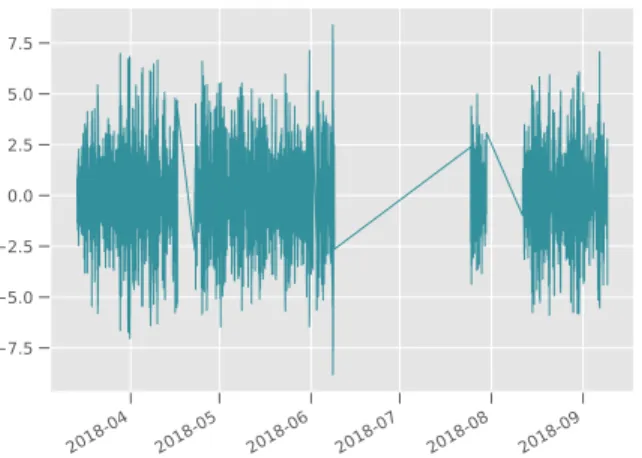
3.2 Simulated Data 30 2018-04 2018-05 2018-06 2018-07 2018-08 2018-09 7.5 5.0 2.5 0.0 2.5 5.0 7.5

Figure 7: Simulated data: AR(1) process withφ = 0.9 and irregular sampling frequencies.

2018-04 2018-05 2018-06 2018-07 2018-08 2018-09 Time 7.5 5.0 2.5 0.0 2.5 5.0 7.5 10.0

(a) Complete simulated time series with outliers

2018-06-052018-06-192018-07-032018-07-172018-07-312018-08-142018-08-282018-09-11 Time 7.5 5.0 2.5 0.0 2.5 5.0 7.5 10.0

(b) Zoom in: Test data with outliers Figure 8: Simulated data: AR(1) process with φ = 0.9. The manually added outliers are highlighted by a red star.

series, one of them shown in Figure 7.

Subsequently, each simulated time series was divided into a training and a test data set. To the test data, five outliers in terms of the PAV algorithm were injected, i.e. data points were added, which lead to a linear pattern with a slope and a length that have not yet occurred in the complete simulated time series. The result for this approach is demonstrated in Figure 8. All other simulated data can be found in the appendix.

4. BASELINE METHODS FOR ANOMALY DETECTION 31

4

Baseline Methods for Anomaly Detection

This Chapter provides a conceptual introduction on the methods that were identified to be suitable to serve as a baseline. These baseline methods originate from traditional Statistical Process Control (SPC) and have been adapted in a way that they suit the task of unsupervised anomaly detection on unevenly spaced time series. These methods include the 3σ-rule (Chapter4.1), a modification of the 3σ-rule based on a rolling average (Chapter 4.2), the exponentially weighted moving average (EWMA) (Chapter4.3) and an approach based on percentiles (Chapter 4.4).

4.1

The

3

σ

-Rule

In many applications, anomaly detection is based on statistical properties, like mean, median, mode, percentiles and standard deviations (Choudhary, 2017). Particularly, the field of Statistical Process Control (SPC), which is closely related to univariate outlier detection (Ben-Gal,2005), makes use of these statistical properties to monitor the quality of a manufacturing or a business process. SPC was pioneered by Walter A. Shewhart in the 1920s. He developed the concept of statistical control and the control chart, which is nowadays also called the Shewhart chart. A stable process, or in other words a process in statistical control, displays variation that is natural to the process, i.e. has common sources of variation. On the other hand, a process, which would be identified as being not in statistical control, displays special sources of variation. This variation either originates from assignable sources or the variation is indicative of a change in the process. A control chart is a map of quality features or a map of statistics of these quality features computed from a sample of measurements. Periodically, a sample is taken (e.g. a sample of products) and quality features, such as the fraction of defective products, are computed. Then, the value of the quality feature itself or a statistic thereof (e.g. the mean of the features) are mapped on the y-axis of a two-dimensional coordinate system. The horizontal axis refers to the time point when the sample was taken. Furthermore, a center line and a symmetric upper and lower control limit (see Figure 9) are drawn. In most use cases, the value of the center line and the control limits are computed based on the average and the standard deviation of historic samples, when the process was labeled to be in statistical control. The con