1
DeepGraphMolGen,
a
multi-objective,
computational
strategy for generating molecules with desirable properties:
a graph convolution and reinforcement learning approach
1,2Yash Khemchandani, 3Stephen O’Hagan, 1Soumitra Samanta, 1Neil Swainston, 1Timothy J. Roberts, 4Danushka Bollegala & 1,5,*Douglas B. Kell1Department of Biochemistry and Systems Biology, Institute of Systems, Molecular and Integrative Biology, University of Liverpool, Crown St, Liverpool L69 7ZB, UK.
2Indian Institute of Technology Bombay, Powai, Mumbai 400 076, Maharashtra, India
3Dept of Chemistry, Manchester Institute of Biotechnology, The University of Manchester, 131 Princess St, Manchester M1 7DN, UK.
4Dept of Computer Science, University of Liverpool, Ashton Building, Ashton Street, Liverpool, L69 3BX, UK.
5The Novo Nordisk Foundation Center for Biosustainability, Technical University of Denmark, Kemitorvet 200, 2800 Kgs Lyngby, Denmark.
*Correspondence: Douglas B. Kell, [email protected] http://dbkgroup.org/ @dbkell
Keywords: Cheminformatics – deep learning – generative methods – QSAR – reinforcement learning
2
DeepGraphMolGen, a multi-objective, computational strategy for generating
molecules with desirable properties: a graph convolution and reinforcement learning
approach ... 1
Abstract ... 2
1 Introduction ... 3
2. Methods ... 4
2.1 Molecular Property Prediction ... 5
2.1.1 Feature Extraction ... 5
2.1.2 Regression ... 6
2.2 Reinforcement Learning for Molecular Generation ... 7
2.2.1 Molecular Representation ... 8
2.2.2 Reinforcement Learning setup ... 8
2.2.3 Graph Convolutional Policy Network ... 9
2.2.4 Policy Gradient Training ... 10
3. System evaluation ... 11
3.1 Property Prediction ... 11
3.1.1 Hyperparameter Optimization ... 12
3.1.2 Implementation details ... 13
3.2 Single-Objective Molecular Generation ... 13
3.3 Multi-Objective Molecular Generation ... 18
Conclusions ... 20
Acknowledgments ... 20
References ... 20
Abstract
We address the problem of generating novel molecules with desired interaction properties as a multi-objective optimization problem. Interaction binding models are learned from binding data using graph convolution networks (GCNs). Since the experimentally obtained property scores are recognised as having potentially gross errors, we adopted a robust loss for the model. Combinations of these terms, including drug likeness and synthetic accessibility, are then optimized using reinforcement learning based on a graph convolution policy approach. Some of the molecules generated, while legitimate chemically, can have excellent drug-likeness scores but appear unusual. We provide an example based on the binding potency of small molecules to dopamine transporters. We extend our method successfully to use a multi-objective reward function, in this case for generating novel molecules that bind with dopamine transporters but not with those for norepinephrine. Our method should be generally applicable to the generation in silico of molecules with desirable properties.
3
1 Introduction
The in silico (and experimental) generation of molecules or materials with desirable properties is an area of immense current interest (e.g. [1-28]). However, difficulties in producing novel molecules by current generative methods arise because of the discrete nature of chemical space, as well as the large number of molecules [29]. For example, the number of drug-like molecules has been estimated to be between 1023 and 1060 [30-34]. Moreover, a slight change in molecular structure can lead to a drastic
change in a molecular property such as binding potency (so-called activity cliffs [35-37]).
Earlier approaches to understanding the relationship between molecular structure and properties used methods such as random forests [38, 39], shallow neural networks [40, 41], Support Vector Machines [42], and Genetic Programming [43]. However, with the recent developments in Deep Learning [44, 45], deep neural networks have come to the fore for property prediction tasks [3, 46-48]. Notably, Coley et al. [49]] used Graph convolutional networks effectively as a feature encoder for input to the neural network.
In the past few years, there have been many approaches to applying Deep Learning for molecule generation. Most papers use the Simplified Molecular-Input Line-Entry System (SMILES) strings as inputs [50], and many use a Variational AutoEncoder architecture (e.g. [3, 17, 51]), with Bayesian Optimization in the latent space to generate novel molecules. However, the use of a sequence-based representational model has a specific difficulty, as any method using them has to learn the inherent rules, in this case of SMILES strings. More recent approaches, such as Grammar Variational AutoEncoders [52, 53] have been developed in attempts to overcome this problem but still the molecules generated are not always valid. Some other approaches try to use Reinforcement Learning for generating optimized molecule [54]. However, they too make use of SMILES strings which as indicated poses a significant problem. In particular, the SMILES grammar is entirely context-sensitive: the addition of an extra atom or bracket can change the structure of the encoded molecule dramatically, and not just ‘locally’ [55].
Earlier approaches have tended to choose a specific encoding for the molecules to be used as an input to the model, such as one hot encoding [56, 57], Extended Connectivity Fingerprints [58, 59] and Generative Examination Networks [60] use SMILES strings directly. We note that these encodings do not necessarily capture the features that need to be obtained for prediction of a specific property (and all encodings extract quite different and orthogonal features [61]).
In contrast, the most recent state-of-the-art methods, including hypergraph grammars [62], Junction Tree Variational Auto Encoders [63] and Graph Convolutional Policy Networks [34], use a graphical representation of molecules rather than SMILES strings and have achieved 100% validity in molecular generation. Graph-based methods have considerable utlility (e.g. [64-70] and can be seen as a more natural representation of molecules as substructures map directly to subgraphs, but subsequences are usually meaningless. However, these have only been used to compare the models on deterministic properties such as the Quantitative Estimate of Drug-likeness (QED) [71], logP, etc. that can be calculated directly from molecular structures (e.g. Using RDKit, http://www.rdkit.org/). For many other applications, molecules having a higher score for a specific measured property are more useful. We here try to tackle this problem.
4
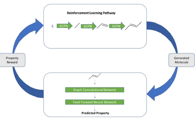
Figure 1. Block diagram of our basic system. A molecule is generated by the Reinforcement Learning (RL) pathway using a Graph Convolutional Policy Networks. This molecule is then used as an input for the property prediction module which outputs the property score as predicted by the module. This score is then used as the reward feedback for the RL pathway and the cycle restarts
2. Methods
Our system consists of two parts: Property Prediction and Molecular Generation. For both the parts, we represent the molecules as graphs [72] since they are a more natural representation than are SMILES strings, and substructures are simply subgraphs. We train a model to predict the property scores of the molecules, specifically the binding constant of various molecules at the dopamine and norepinephrine transporters (using a dataset from BindingDB). The first part, used for (training) the property prediction part, is a Graph Convolutional Network as a feature encoder together with a Feed Forward Network. We also use an Adaptive Robust Loss Function (as suggested by [73]) since the experimental data are bound to be error prone. For the Molecular Generation task, we use the method proposed by You and colleagues [34]. In particular, we (and they) use Reinforcement Learning for this task since it allows us to incorporate both the molecular constraints and the desired properties using reward functions. This part uses graph convolution policy networks (GCPNs), a model consisting of a GCN that predicts the next action (policy) given the molecule state. It is further guided by expert pretraining and adversarial loss for generating valid molecules. Our code (https://github.com/dbkgroup/prop_gen) is essentially an integration of the property prediction code of Yang and colleagues [74, 75] (https://github.com/swansonk14/chemprop) and the reinforcement learning code provided by You and colleagues [34].
5
2.1 Molecular Property Prediction
As noted, the supervised property prediction model consists of a graph-convolution network for feature extraction followed by a fully interconnected feedforward network for property prediction.
2.1.1 Feature Extraction
We represent the molecules as directed graphs, with each atom (𝑖) having a feature vector 𝐹𝑖(ℝ133)
and each bond (between atom 𝑖 & 𝑗) having feature vector𝐹𝑖𝑗(ℝ14 ). For each incoming bond a
feature vector is obtained by concatenating the feature vector of the atom to which the bond is incoming and the feature vector of the bond. Thus the input tensor is of the size 𝑁bonds x ℝ147 . The
Graph Convolution approach allows the message (feature vector) for a bond to be passed around the entire graph using the approach described below.
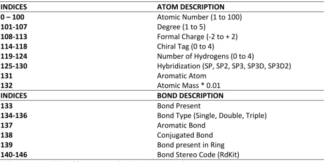
The initial atom-bond feature vector that we use incorporates important molecular information that the GCN encoder can then incorporate in later layers. The initial representations for the atom and bond features are taken from https://github.com/swansonk14/chemprop and summarized in Table 1, below. Each descriptor is a one-hot vector covering the index-range represented by it (except the Atomic Mass). For Atomic Number, Degree, Formal Charge, Chiral Tag, Number of Hydrogens and Hybridization, the feature vector contains one additional dimension to allow uncommon values (values not in the specified range).
INDICES ATOM DESCRIPTION
0 – 100 Atomic Number (1 to 100) 101-107 Degree (1 to 5) 108-113 Formal Charge (-2 to + 2) 114-118 Chiral Tag (0 to 4) 119-124 Number of Hydrogens (0 to 4) 125-130 Hybridization (SP, SP2, SP3, SP3D, SP3D2) 131 Aromatic Atom 132 Atomic Mass * 0.01
INDICES BOND DESCRIPTION
133 Bond Present
134-136 137
Bond Type (Single, Double, Triple) Aromatic Bond
138 Conjugated Bond
139 Bond present in Ring
140-146 Bond Stereo Code (RdKit)
Table 1. Atom and bond features used in the present work
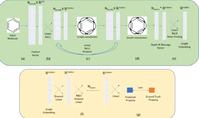
The initial atom-bond feature vector is then passed through a linear layer followed by ReLU Activation [76, 77] to get the Depth-0 message vector for each bond. For each bond, the message vectors for the neighbouring bonds are summed up (Convolution step) and passed through a linear layer followed by ReLU and a Dropout layer to get the Depth-1 message vectors. This process is continued up to a specified Depth-(N-1) message vectors. To get the Depth-N message vectors, the Depth-(N-1) vectors of all the incoming bonds for an atom are summed and then passed through a dense layer followed by ReLU and Dropout. The final graph embedding for the molecule is obtained by averaging the depth-N message vectors over all the atoms. The exact details for this model can be found in section 3.1.1.
6
Figure 2. The property prediction pipeline for our method. The steps in green represent the feature extraction using Graph Convolution and the steps in orange represent regression of property scores. (a) The molecule is represented is a feature vector with features described as in section 2.1. (b) The feature vector is passed through a linear layer to get Depth-0 message. (c) Through repeated graph convolution (message passing) followed by Linear Layer, we get Depth N-1 message. (d) Each atom’s final message is calculated by summing up the messages (also Graph Convolution) of the neighbouring atoms. (e) The resultant message is passed through a Linear Layer and the mean of all the atoms is taken to get the final embedding. (f) The property score is regressed from the graph embedding by a Feed Forward Neural Network. (g) The loss between predicted property and ground truth property is then backpropagated to change the weights.
2.1.2 Regression
To perform property prediction the embedding extracted by the GCN is fed into a fully connected network. Each intermediate layer consists of a Linear Layer followed by ReLU activation and Dropout that map the hidden vector to another vector of the same size. Finally the penultimate nodes are passed through a Linear Layer to output the predicted property score. The Ki values present in the
dataset were obtained experimentally so might contain experimental errors. If we were to train our model with a simple loss function such as root mean square (RMS) error loss, it would not be able to generalize well because of the presence of outliers in the training set. Overcoming this problem requires training the data with the help of a robust loss function that takes care of the outliers present in the training data. There are several types of robust loss functions such as Pseudo-Huber loss [78], Cauchy loss, etc., but each of them has an additional hyperparameter value (for example δ in Huber Loss) which is treated as a constant while training. This means that we have to manually tune the hyperparameter each time we train to get the optimum value which may result in extensive training time. To overcome this problem , as proposed by [73], we have used a general robust loss function
7
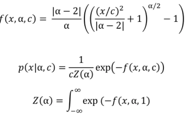
that has the hyperparameters as shape parameter (α) which controls the robustness of the loss, and the scale parameter (c) which controls the size of the loss’s quadratic bowl near x=0. This loss is dubbed as a “general” loss since it takes the form of other loss functions for particular values of α. (e.g L2 loss for α=2, Charbonnier loss for α=1, Cauchy loss for α=0). The authors also propose that “by viewing the loss function as the negative log likelihood of a probability distribution, and by treating robustness of the distribution as a latent variable” we can use gradient-based methods to maximize the likelihood without manual parameter tuning. In other words, we can now train the hyperparameters α and c rather which overcomes the earlier problem of manually tuning the hyperparameters. The loss function and the corresponding probability distribution are described in Eq. 1 and Eq. 2 respectively.
𝑓(𝑥, α, 𝑐) = |α − 2| α (( (𝑥/𝑐)2 |α − 2|+ 1) α/2 − 1) Eq. 1 𝑝(𝑥|α, 𝑐) = 1 𝑐𝑍(α)exp(−𝑓(𝑥, α, c)) 𝑍(α) = ∫ exp (−𝑓(𝑥, α, 1) ∞ −∞ Eq. 2
2.2 Reinforcement Learning for Molecular Generation
We follow the method described by the GCPN paper [34] for the molecular generation task, with the difference being that the final property reward is the value calculated by the previously trained model for the newly generated molecules. GCPN is a state-of-the-art molecule generator that utilizes Proximal Policy Optimization (PPO) as a Reinforcement Learning paradigm for generating molecules. A comparison of GCPN with other generative approaches can be found in Table 2 and Table 3 which compare the ability of generators to produce molecules having higher property scores and targeted property scores, respectively. Note that even though we have chosen GCPN for the molecule generation pipeline, our strategy can be implemented using any graph-based Reinforcement Learning generator since we just need to use the predicted property score as the reward function.
Method Penalized logP QED
1st 2nd 3rd Validity 1st 2nd 3rd Validity
ZINC 4.52 4.30 4.23 100% 0.948 0.948 0.948 100%
ORGAN 3.63 3.49 3.44 0.4% 0.896 0.824 0.820 2.2%
JT-VAE 5.30 4.93 4.49 100% 0.925 0.911 0.910 100%
GCPN 7.98 7.85 7.80 100% 0.948 0.947 0.946 100%
Table 2: Comparison of the top 3 property scores of generated molecules found by each model. Validity is defined as the fraction of generated molecules that are chemically valid. ORGAN and JT-VAE are described in [79] and [63], respectively.
8
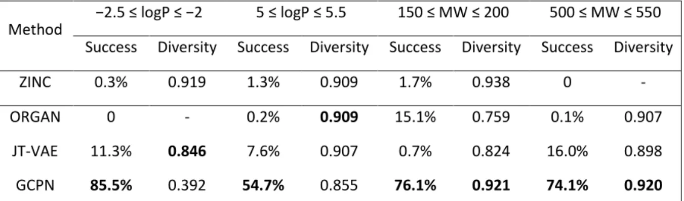
Method −2.5 ≤ logP ≤ −2 5 ≤ logP ≤ 5.5 150 ≤ MW ≤ 200 500 ≤ MW ≤ 550 Success Diversity Success Diversity Success Diversity Success Diversity
ZINC 0.3% 0.919 1.3% 0.909 1.7% 0.938 0 -
ORGAN 0 - 0.2% 0.909 15.1% 0.759 0.1% 0.907
JT-VAE 11.3% 0.846 7.6% 0.907 0.7% 0.824 16.0% 0.898
GCPN 85.5% 0.392 54.7% 0.855 76.1% 0.921 74.1% 0.920
Table 3: Comparison of the effectiveness of property targeting task. MW here stands for the Molecular Weight. Success is defined as the percentage of generated molecules in the target range and Diversity is defined as the average pairwise Tanimoto distance between the Morgan fingerprints of the molecules. Citations to ORGAN and JT-VAE are given in the legend to Table 2.
2.2.1 Molecular Representation
As in the previous part, we represent the molecules as graphs, more specifically as (𝐴, 𝐸, 𝐹) where 𝐴 ∈ {0, 1}𝑛×𝑛 is the adjacency matrix, 𝐹 ∈ ℝ𝑛×𝑑 is the node (atom) feature matrix and 𝐸 ∈ {0, 1}3×𝑛×𝑛 is the edge-conditioned adjacency tensor (since the number of bond-types is 3, namely
single, double and triple bond), with 𝑛 being the number of atoms and 𝑑 being the length of feature vector for each atom. More specifically, 𝐸𝑖,𝑗,𝑘= 1 if there exists a bond of type 𝑖 between atoms 𝑗
and 𝑘 , and 𝐴𝑗,𝑘= 1 if there exists any bond between atoms 𝑗 and 𝑘.
2.2.2 Reinforcement Learning setup
Our model environment builds a molecule step by step with the addition of a new bond in each step. We treat graph generation as a Markov Decision Process such that the next action is predicted based only on the current state of the molecule, not on the path that the generative process has taken. This reduces the need for sequential models such as RNNs and the disadvantages of vanishing gradients associated with them, as well as reducing the memory load on the model. More specifically, the decision process follows the equation: 𝑝(𝑠𝑡+1|𝑠𝑡, . . . 𝑠0) = 𝑝(𝑠𝑡+1|𝑠𝑡), where p is the probability of
next state (𝑠𝑡+1) given the previous state (𝑠𝑡).
We can initialize the generative process with either a single C atom (as in Experiments 1 and 2) or with another molecule (as in Experiments 3, 4 and 5). At any point in the generation process, the state of the environment is the graph of the current molecule that has been built up so far. The action space is a vector of length 4 which contains the information – First Atom, Second Atom, Bond type and Stop. The stop signal is either 0 or 1 indicating whether the generation is complete, based on valence rules. If the action defies the rules of chemistry in the resultant molecule, the action is not considered and the state remains as it is.
We make use of both intermediate and final rewards to guide the decision-making process. The intermediate rewards include stepwise validity checks such that a small constant value is added to the reward if the molecule passes the valency checks. The final reward includes the pKi value of the final
9
and +1 for absence of functional groups that violate ZINC functional group filters). Two other metrics are the quantitative estimation of drug-likeness (QED) [71] and the synthetic accessibility (SA) [80] score. Since our final goal is to generate drug-like molecules that can be synthetically generated, we also add the QED and 2*SA score of the final molecule to the reward.
Apart from this, we also use adversarial rewards so that the generated molecules resemble
(prediction) the given set of molecules (real). We define the adversarial rewards 𝑉(𝜋𝛳, 𝐷Ф) in Eq 3. min
𝜃 max𝜙 𝑉(𝜋𝜃, 𝐷𝜙) = 𝐸𝑥∼𝑝data[log𝐷𝜙(𝑥)] + 𝐸𝑥∼𝜋𝜃[log𝐷𝜙(1 − 𝑥)] Eq. 3
where 𝜋𝜃 is the policy network, 𝐷𝜑 is the discriminator network, 𝑥 represents the input graph and 𝑝data is the underlying data distribution which is defined either over final graphs (for final rewards) or
intermediate graphs (for intermediate rewards) (just as proposed by You and colleagues [34]). Alternate training of generator (policy network) and discriminator by gradient descent methods will not work in our case since 𝑥 is a non-differentiable graph object. Therefore we add – 𝑉(𝜋𝛳, 𝐷Ф) to
our rewards and use policy gradient methods [81] to optimize the total rewards. The discriminator network comprises a Graph Convolutional Network for generating the node embedding and a Feed Forward Network to output whether the molecule is real or fake. The GCN mechanism is same as that of the policy network which is described in the next section.
2.2.3 Graph Convolutional Policy Network
We use Graph Convolutional Networks (GCNs) as the policy function for the bond prediction task. This variant of graph convolution performs message passing over each edge type for a fixed depth 𝐿. “The node embedding for the next depth (𝑙 + 1) is calculated as described in Eq. 4
where 𝐸𝑖 is the 𝑖𝑡ℎ slice of the tensor 𝐸, 𝐸̃𝑖 = 𝐸𝑖+ 𝐼, 𝐷̃𝑖 = ∑ 𝐸̃𝑘 𝑖𝑗𝑘, 𝑊𝑖 (𝑙)
is a trainable weight matrix for the 𝑖𝑡ℎ edge type, and 𝐻(𝑙)is the node embedding learned in the 𝑙𝑡ℎ layer with 𝐻(𝑙) ∈ ℝ(𝑛+𝑐)×𝑑
[34]. 𝑛 is the number of atoms in the current molecule and 𝑐 is the number of possible atom types (C,N,O etc.) that can be added to the molecule (one atom is added in each step) with 𝑑 representing the dimension of the embedding. We use mean over the edge features as the Aggregate (AGG) function to obtain the node embedding for a layer. This process is repeated 𝐿 times until we get the final node embedding.
This node embedding 𝑋 is then used as the input to four Multilayer Perceptrons (MLP, denoted by 𝑚), that map a matrix 𝑍 ∈ℝ𝑝×𝑑to ℝ𝑝representing the probability of selecting a particular entity from
the given 𝑝 entities. The specific entity is then sampled from the probability distribution thus obtained. Note that since the action space is a vector of length 4, we use 4 perceptrons to sample each
𝐻(𝑙+1) = AGG (ReLU ({𝐷̃𝑖 −1 2𝐸̃ 𝑖𝐷̃𝑖 −1 2𝐻(𝑙)𝑊 𝑖 (𝑙) }, ∀𝑖 ∈ (1, … , 𝑏))) Eq. 4
10
component of the vector. The first atom has to be from the current molecule state while the second atom can be from the current molecule (forming a cycle) or a new atom outside the molecule (adding a new atom). For selecting the first atom, the original embedding 𝑋 is passed to the MLP 𝑚𝑓and
outputs a vector of length equal to 𝑛. While selecting the second atom, the embedding of first atom
𝑋𝑎firstis concatenated to the original embedding 𝑋 and passed to the MLP 𝑚𝑠 giving a vector of length
equal to 𝑛 + 𝑐. While selecting the edge type, the concatenated embedding of the first (𝑋𝑎first) and
second (𝑋𝑎second) atom is used as an input to MLP 𝑚𝑒 and outputs a vector of length equal to 3
(number of bond types). Finally, the mean embedding of the atoms is passed to MLP 𝑚𝑡 to output a
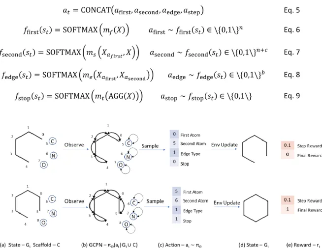
vector of length 2 indicating whether to stop the generation. This process is described in equations 5-9.
Figure 3. The reinforcement learning pathway for systemic generation of molecules (Redrawn from You et al. [34]) . (a) The state is defined as the current graph 𝐺𝑡 and the possible atom types 𝐶. (b) The
GCPN conducts message passing to encode the state as node embeddings and estimates the policy function. (c) The action to be performed (𝑎𝑡) is sampled from the policy function. The environment
performs a chemical valency check on the intermediate state and returns (d) the next state 𝐺𝑡 and (e)
the associated reward (𝑟𝑡)
2.2.4 Policy Gradient Training
For our experiments, we use Proximal Policy Optimization (PPO) [81], the state-of-the-art policy gradient method, for optimizing the total reward. The objective function for PPO is described in Eq 10.
𝑎𝑡 = CONCAT(𝑎first, 𝑎second, 𝑎edge, 𝑎step) Eq. 5
𝑓first(𝑠𝑡) = SOFTMAX (𝑚𝑓(𝑋)) 𝑎first∼ 𝑓first(𝑠𝑡) ∈ \{0,1\}𝑛 Eq. 6
𝑓second(𝑠𝑡) = SOFTMAX (𝑚𝑠(𝑋𝑎𝑓𝑖𝑟𝑠𝑡, 𝑋)) 𝑎second∼ 𝑓second(𝑠𝑡) ∈ \{0,1\}𝑛+𝑐 Eq. 7
𝑓edge(𝑠𝑡) = SOFTMAX (𝑚𝑒(𝑋𝑎first, 𝑋𝑎second)) 𝑎edge∼ 𝑓edge(𝑠𝑡) ∈ \{0,1\}
𝑏 Eq. 8 𝑓stop(𝑠𝑡) = SOFTMAX (𝑚𝑡(AGG(𝑋))) 𝑎stop ∼ 𝑓stop(𝑠𝑡) ∈ \{0,1\} Eq. 9
11
Here 𝑠𝑡, 𝑎𝑡, 𝑅𝑡 are the state, action and reward respectively at timestep 𝑡, 𝑉(𝑠𝑡) is the value associated
with state 𝑠𝑡, 𝜋𝜃 is the policy function and 𝛾 is the discount factor. Also note that 𝐴̂𝑡, which is an
estimator of the advantage function at timestep 𝑡, has been estimated using Generalized Advantage Estimation [82] with the GAE parameter 𝜆, since it reduces the variance of the estimate.
For estimating the value of 𝑉 we use an MLP with the embedding 𝑋 as the input. Apart from this, we also use expert pretraining [83] which has shown to stabilise the training process. For our experiment, any ground truth molecule can be used as an expert for imitation. We randomly select a subgraph 𝐺̂’
from the ground truth molecule 𝐺 ̂as the state 𝑠̂𝑡. The action 𝑎̂𝑡is also chosen randomly such that it
adds an atom or bond in the graph 𝐺̂\𝐺̂’ . This pair (𝑠̂𝑡, 𝑎̂𝑡) is used for calculating the expert loss.
min𝐿EXPERT(𝜃) = −log(𝜋
𝜃(𝑎̂𝑡|𝑠̂𝑡)) Eq. 11
Note that we use the same dataset of ground truth molecules for calculating the expert loss and the adversarial rewards. For the rest of the paper, we will call this dataset the “expert dataset” and the random molecule selected from the dataset the “expert molecule”.
3. System evaluation
In this section we evaluate the system described above on the task of generating small molecules that interact with the dopamine transporter but not (so far as possible) with the norepinephrine transporter.
3.1 Property Prediction
In this section we evaluate the performance of the supervised property prediction component. Dopamine Transporter binding data was obtained from www.bindingdb.org (https://bit.ly/2YACT5u). The training data consist of some molecules which are labelled with their Ki values and some which
are labelled with IC50 values. For this paper, we have used IC50 values and Ki values interchangeably in
order to increase the size of the training dataset. Molecules having large Ki values in the dataset were
not labelled accurately (with labels such as ~1000) but the use of a robust loss function allowed us to incorporate these values directly. As stated above we use log transformed values (pKi). (We also attempted to learn the Ki values of the molecules, but the distribution was found to be
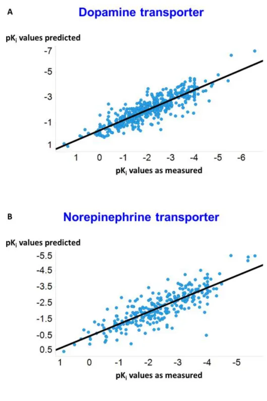
heteroscedastic; hence we focus on predicting the pKi values.) Data are shown in Fig 4A for the
dopamine transporter and 4B for the norepinephrine transporter pKi values.
max𝐿CLIP(𝜃) =𝔼 𝑡[min(𝑟𝑡(𝜃)𝐴̂𝑡,clip(𝑟𝑡(𝜃), 1 − 𝜖, 1 + 𝜖)𝐴̂𝑡)] 𝑟𝑡(𝜃) = 𝜋𝜃(𝑎𝑡|𝑠𝑡) 𝜋𝜃old(𝑎𝑡|𝑠𝑡) 𝐴̂𝑡 = 𝛿𝑡+ (𝛾𝜆)𝛿(𝑡+1)+ ⋯ + (𝛾𝜆)𝑇−𝑡+1𝛿𝑇−1 where 𝛿𝑡 = 𝑅𝑡+ 𝛾𝑉(𝑠𝑡+1) − 𝑉(𝑠𝑡) Eq. 10
12
Figure 1 : Predicted and experimental values for the test sets of the dopamine (A) and norepinephrine (B) transporters. Lines are lines of best fit (A: y =0.44 + 0.79x, r2 = 0.79; B: y = 0.49 + 0.74x, r2 =0.68).
3.1.1 Hyperparameter Optimization
As the property prediction is a general algorithm with a large number of hyperparameters, we attempted to improve generalisation on the transporter problem using Bayesian optimization on the RMSE error between the predicted pKi values and the actual pKi values of the validation set. For this task we consider the hyperparameters to be the depth of the GCN encoder, the dimensions of the
13
message vectors, the number of layers in the Feed Forward Network, and the Dropout constant. We use 10-fold cross validation on the train and validation dataset with the test set held out. The model score is defined as the mean RMS error of the 10 folds and we use Bayesian optimization to minimize the model score.
For the case of the dopamine transporter, the optimum hyperparameters that were obtained are 3 (depth of GCN), 1300 (dimensions of message vector), 2 (FFN layers) and 0.1 (Dropout).The RMS error on the test dataset for the dopamine transporter after Hyperparameter Optimization was found to be 0.57 as compared to an error of 0.65 without it. We attribute this quite significant remaining error to the errors present in the dataset. Similarly for the norepinephrine transporter , the test RMS error was found to be 0.66 after hyperparameter optimization and the optimum hyperparameters obtained are 5 (depth of GCN), 900 (dimensions of message vector), 3 (FFN layers), 0.15 (Dropout).
3.1.2 Implementation details
For the prediction of pKi value of both Dopamine and Norepinephrine transporters, we split the overall dataset into train (80%) , validation (10%) and test (10%) datasets randomly. The training is done with a batch size of 50 molecules and for 100 epochs. All the network weights were initialized using Xavier initialization [84]. The first two epochs are warmup epochs [85] where the learning rate increases from 1e-4 to 1e-3 linearly and after that it decreases exponentially to 1e-4 by the last epoch. The model is saved after an epoch if the RMS error on the validation dataset is less than the previous best and the error for the test dataset is calculated using the saved model which has the least error on the validation dataset. The code was written in PyTorch library and the training was done using an NVIDIA RTX 2080Ti GPU on a Windows 10 system with 256GB RAM and Intel 18-Core Xeon W-2195 processor.
3.2 Single-Objective Molecular Generation
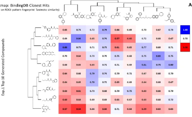
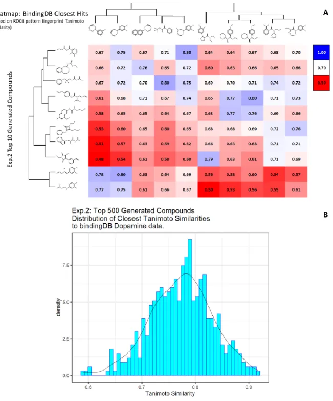
To begin the RL evaluation we consider molecular generation with a single objective (dopamine transporter interaction). For all the experiments we use the following implementation details. The learning rate for training all the networks is taken to be 1e-3 and linearly decreasing to 0 by 3e7 timesteps. The depth of GCN network for both the GCPN and the Discriminator network is taken to be 3 and the node embedding size was taken to be 128. The code was written using the TensorFlow library and training was done using an NVIDIA RTX 2080Ti GPU as per the previous paragraph. For the task of analysing the results we provide the ‘top 10’ molecules generated as in Fig 5. However, we aim to generate molecules that are in some sense similar to the original training dataset by systematically modifying the RL pathway in the following experiments. For each experiment, we find the closest molecule in the BindingDB dataset to the top 10 generated molecules. The relative closeness is measured by calculating its Tanimoto Similarity between the RDKit fingerprints and visualize the distribution of the TS values.
First, we initialize the molecule with a single Carbon atom in the beginning of the generative process. The expert dataset in this case is chosen to be the ZINC dataset [86], which is a free dataset containing (at that time) some 230M commercially available compounds. However, for our experiments, we use 250K randomly selected molecules from ZINC as our expert dataset to make the experiments computationally tractable. The top generated molecules and their predicted properties are given in Supplementary Table 1 (including data on QED and SA) with a subset of the data illustrated in Fig 5. Note that in all cases the values of QED and SA both exceeded 0.8.
14
Figure 5. In silico generation by DeepGraphMolGen of novel molecules with predicted binding capacity to the dopamine transporter. Molecules were generated as described in the text. A. Top 10 molecules as predicted by DeepGraphMolGen versus the closest molecule in the BindingdB dataset and the Tanimoto similarity thereto (encoded using the RDKit patterned fingerprint). B. Distribution of Tanimoto similarities to a molecule in BindingdB dataset of the top 500 molecules.
Although the above experiment was able to generate optimized molecules, there is no certainty that the predictions are correct due to the errors in the model as well as the errors that were propagated by the experimental errors in the data. We thus attempt to generate molecules that are similar to the more potent molecules. In the next experiment, we choose the expert dataset to be the original
15
dataset on which we trained the molecules (we will call this the Dopamine Dataset), while omitting molecules having Ki greater than 1000. We again choose the initial molecule to be a single carbon
atom. The equivalent data are given in Supplementary Table 2, with similar plots to those of Fig 5 given in Fig 6.
Figure 6. In silico generation by DeepGraphMolGen of novel molecules with predicted binding capacity to the dopamine transporter. Molecules were generated as described in the text. A. Top 10 molecules as predicted by DeepGraphMolGen versus the closest molecule in the BindingdB dataset and the Tanimoto similarity thereto (encoded using the RDKit patterned fingerprint). B. Distribution of Tanimoto similarities to a molecule in BindingdB dataset of the top 500 molecules.
16
Another way to ensure that the generated molecules will have a high affinity towards dopamine transporter is to explicitly ensure that the molecules have higher TS with already known molecules that have high pKi values. We attempt to achieve this by initializing the generative process with a
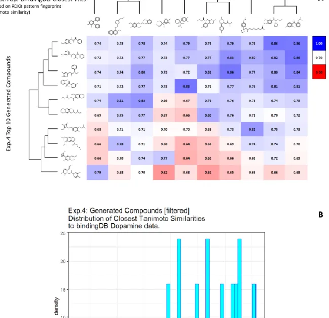
random molecule from the Dopamine Dataset having Ki < 1000. We conduct two experiments using this process, one where we restrict the number of atoms (other than hydrogen) to be lower than 25 (Supplementary Table 3 and Fig 7), and another ( Supplementary Table 4 and Fig 8) where we restrict the number of atoms to be less than 15. For both these experiments, we use the ZINC dataset as the expert dataset. The results are summarized in the tables below. Note that in some cases we obtain a TS of 1; this is encouraging as in this case the algorithm found no need to add anything to the original molecule and could recapitulate it.
17
Figure 7. In silico generation by DeepGraphMolGen of novel molecules with predicted binding capacity to the dopamine transporter using a generative method in which the number of heavy atoms is constrained to be lower than 25. Molecules were generated as described in the text. A. Top 10 molecules as predicted by DeepGraphMolGen versus the closest molecule in the BindingdB dataset and the TS thereto (encoded using the RDKit patterned fingerprint). B. Distribution of Tanimoto similarities (RDKit patterned encoding) to a molecule in BindingdB dataset of the top 500 molecules.
Figure 8. In silico generation by DeepGraphMolGen of novel molecules with predicted binding capacity to the dopamine transporter using a generative method in which the number of heavy
18
atoms is constrained to be lower than 15. Molecules were generated as described in the text. A. Top 10 molecules as predicted by DeepGraphMolGen versus the closest molecule in the BindingdB dataset and the TS thereto (encoded using the RDKit patterned fingerprint). B. Distribution of Tanimoto similarities (RDKit patterned encoding) to the closest molecule in BindingdB dataset of the top 500 molecules.
3.3 Multi-Objective Molecular Generation
Even though generating molecules having higher affinity towards a particular ligand in itself is quite sought after, in many cases we might wish to seek molecules that bind to one receptor but explicitly do not bind to another one (kinase inhibitors might be one such example). We attempt to achieve this here with the help of our Reinforcement Learning pipeline by modifying the reward function to be a weighted combination of pKi values for the two different targets. Explicitly, we attempt to generate
molecules that have high binding affinity to the Dopamine Transporter but a much lower binding affinity to the Norepinephrine Transporter. Thus, we modify the reward function used in the previous experiments to add 2 times the predicted pKi values for Dopamine Transporter and -1 times the
predicted pKi values for the Norepinephrine Transporter. The higher weight is given to the dopamine
component since we wish to generate molecules that do bind to it. Clearly we could use any other weightings as part of the reward function, so those chosen are simply illustrative. For this experiment we initialize the process with a random molecule from the Dopamine dataset having a number of atoms lower than 25 and choose the expert dataset to be ZINC. The results of this experiment are summarized in Supplementary Table 5 and Fig 9. As above, some molecules have a TS of 1 to examples in the dataset, for the same reasons.
19
Figure 9. In silico generation by DeepGraphMolGen of novel molecules with predicted binding capacity to the dopamine transporter using a generative method in which the number of heavy atoms is constrained to be lower than 25. Molecules were generated as described in the text. A. Top 10 molecules as predicted by DeepGraphMolGen versus the closest molecule in the BindingdB dataset and the TS thereto (encoded using the RDKit patterned fingerprint). B. Distribution of Tanimoto similarities (RDKit patterned encoding) to the closest molecule in BindingdB dataset of the top 500 molecules. C. Plot of those molecules with differential affinities for the dopamine and norepinephrine transporters.
20
Only in rare cases do candidate solutions for multi- (in this case two-)objective optimisation problems have unique solutions that are optimal for both [87], and there is a trade-off that is left to the choice of the experimenter. Thus, Fig 9C also illustrates the molecules on the Pareto front for the two objectives, showing how quite changes in structure can move one swiftly along the Pareto front. Consequently our method also provides a convenient means of attacking multi-objective molecular optimisation problems.
Conclusions
Overall, the present molecular graph-based generative method has a number of advantages over grammar-based encodings, in particular that it necessarily creates valid molecules. As stressed by Coley and colleagues [49], such methods still retain any inherent limitations of 2D methods as a priori
they do not encode 3D information. This said, there is evidence that 3D structures do not add much benefit when forming QSAR models [88-92], so we do not consider this a major limitation for now. Some of the molecules generated might be seen by some (however subjectively) as ‘unusual, even though they scored well on both drug-likeness and synthetic accessibility metrics. This probably says much about the size of plausible drug space that exists relative to the fraction that has actually been explored [93-95], and implies that generative methods can have an important role to play in medicinal chemistry. Also, for generating desired molecules, the QSAR models need to be accurate and robust in order to evaluate accurately the property of the generated molecules. Recent works such as [96] include uncertainty metrics for property discrimination, and benchmarking models are also available [97]. In conclusion, we here add to the list of useful, generative molecular methods for virtual screening by combining molecular graph encoding, reinforcement learning and multi-objective optimisation within a single strategy.
Acknowledgments
The work of SS and DBK is supported as part of EPSRC grant EP/S004963/1 (SuSCoRD).
Conflict of interest statement
The authors have no conflicts of interest to report.
References
1. Yang X, Zhang J, Yoshizoe K, Terayama K, Tsuda K: ChemTS: an efficient python library for de
novo molecular generation. Sci Technol Adv Mater 2017, 18(1):972-976.
2. Gómez-Bombarelli R, Aguilera-Iparraguirre J, Hirzel TD, Duvenaud D, Maclaurin D, Blood-Forsythe MA, Chae HS, Einzinger M, Ha DG, Wu T et al: Design of efficient molecular organic light-emitting diodes by a high-throughput virtual screening and experimental approach.
21
3. Gómez-Bombarelli R, Wei JN, Duvenaud D, Hernández-Lobato JM, Sánchez-Lengeling B, Sheberla D, Aguilera-Iparraguirre J, Hirzel TD, Adams RP, Aspuru-Guzik A: Automatic Chemical
Design Using a Data-Driven Continuous Representation of Molecules. ACS Cent Sci 2018,
4(2):268-276.
4. Sanchez-Lengeling B, Aspuru-Guzik A: Inverse molecular design using machine learning:
Generative models for matter engineering. Science 2018, 361(6400):360-365.
5. Kadurin A, Nikolenko S, Khrabrov K, Aliper A, Zhavoronkov A: druGAN: An advanced
generative adversarial autoencoder model for de novo generation of new molecules with
desired molecular properties in silico. Mol Pharm 2017, 14(9):3098-3104.
6. Olier I, Sadawi N, Bickerton GR, Vanschoren J, Grosan C, Soldatova L, King RD: Meta-QSAR: a
large-scale application of meta-learning to drug design and discovery. Mach Learn 2018,
107(1):285-311.
7. Popova M, Isayev O, Tropsha A: Deep reinforcement learning for de novo drug design. Sci Adv 2018, 4(7):eaap7885.
8. Tabor DP, Roch LM, Saikin SK, Kreisbeck C, Sheberla D, Montoya JH, Dwaraknath S, Aykol M, Ortiz C, Tribukait H et al: Accelerating the discovery of materials for clean energy in the era
of smart automation. Nature Reviews Materials 2018, 3:5-20.
9. Colby SM, Nuñez JR, Hodas NO, Corley CD, Renslow RR: Deep Learning to Generate in Silico Chemical Property Libraries and Candidate Molecules for Small Molecule Identification in
Complex Samples. Analytical chemistry 2020, 92(2):1720-1729.
10. Baskin, II: The power of deep learning to ligand-based novel drug discovery. Expert Opin Drug Discov 2020:1-10.
11. Hong SH, Ryu S, Lim J, Kim WY: Molecular Generative Model Based on an Adversarially
Regularized Autoencoder. J Chem Inf Model 2020, 60(1):29-36.
12. Lim J, Hwang SY, Moon S, Kim S, Kim WY: Scaffold-based molecular design with a graph
generative model. Chem Sci 2020, 11(4):1153-1164.
13. Rifaioglu AS, Nalbat E, Atalay V, Martin MJ, Cetin-Atalay R, Doğan T: DEEPScreen: high performance drug-target interaction prediction with convolutional neural networks using
2-D structural compound representations. Chem Sci 2020, 11(9):2531-2557.
14. Yasonik J: Multiobjective de novo drug design with recurrent neural networks and
nondominated sorting. J Cheminform 2020, 12(1):14.
15. Yoshimori A, Kawasaki E, Kanai C, Tasaka T: Strategies for Design of Molecular Structures with
a Desired Pharmacophore Using Deep Reinforcement Learning. Chem Pharm Bull (Tokyo)
2020, 68(3):227-233.
16. Walters WP, Murcko M: Assessing the impact of generative AI on medicinal chemistry. Nat Biotechnol 2020, 38(2):143-145.
17. Griffiths RR, Hernández-Lobato JM: Constrained Bayesian optimization for automatic
chemical design using variational autoencoders. Chem Sci 2020, 11(2):577-586.
18. Cova TFGG, Pais AACC: Deep Learning for Deep Chemistry: Optimizing the Prediction of
Chemical Patterns. Front Chem 2019, 7.
19. Noh J, Kim J, Stein HS, Sanchez-Lengeling B, Gregoire JM, Aspuru-Guzik A, Jung Y: Inverse
Design of Solid-State Materials via a Continuous Representation. Matter 2019,
1(5):1370-1384.
20. Grisoni F, Schneider G: De novo Molecular Design with Generative Long Short-term Memory.
Chimia 2019, 73(12):1006-1011.
21. Grisoni F, Merk D, Friedrich L, Schneider G: Design of Natural-Product-Inspired Multitarget
Ligands by Machine Learning. ChemMedChem 2019, 14(12):1129-1134.
22. Gupta A, Müller AT, Huisman BJH, Fuchs JA, Schneider P, Schneider G: Generative Recurrent
Networks for de novo drug design. Mol Inform 2018, 37(1-2):1700111.
23. Merk D, Friedrich L, Grisoni F, Schneider G: De Novo Design of Bioactive Small Molecules by Artificial Intelligence. Mol Inform 2018, 37(1-2).
22
24. Schneider G: Generative models for artificially-intelligent molecular design. Mol Inform
2018, 37(1-2):188031.
25. Schneider P, Walters WP, Plowright AT, Sieroka N, Listgarten J, Goodnow RA, Fisher J, Jansen JM, Duca JS, Rush TS et al: Rethinking drug design in the artificial intelligence era. Nat Rev Drug Discov 2020, 19:353-364.
26. Button A, Merk D, Hiss JA, Schneider G: Automated de novo molecular design by hybrid
machine intelligence and rule-driven chemical synthesis. Nat mach Intell 2019, 1(7):307-315.
27. Moret M, Friedrich L, Grisoni F, Merk D, Schneider G: Generative molecular design in low data
regimes. Nat Mach Intell 2020, 2:171-180.
28. Ståhl N, Falkman G, Karlsson A, Mathiason G, Boström J: Deep Reinforcement Learning for
Multiparameter Optimization in de novo Drug Design. J Chem Inf Model 2019,
59(7):3166-3176.
29. Arús-Pous J, Blaschke T, Ulander S, Reymond JL, Chen H, Engkvist O: Exploring the GDB-13
chemical space using deep generative models. J Cheminform 2019, 11(1):20.
30. Reymond JL: The Chemical Space Project. Acc Chem Res 2015, 48(3):722-730.
31. Bohacek RS, McMartin C, Guida WC: The art and practice of structure-based drug design: A
molecular modeling perspective. Med Res Rev 1996, 16(1):3-50.
32. Ertl P: Cheminformatics analysis of organic substituents: identification of the most common substituents, calculation of substituent properties, and automatic identification of drug-like
bioisosteric groups. J Chem Inf Comput Sci 2003, 43(2):374-380.
33. O'Hagan S, Kell DB: Analysing and navigating natural products space for generating small,
diverse, but representative chemical libraries. Biotechnol J 2018, 13(1):1700503.
34. You J, Liu B, Ying R, Pande V, Leskovec J: Graph Convolutional Policy Network for
Goal-Directed Molecular Graph Generation. arXiv 2018:1806.02473v02471.
35. Dimova D, Stumpfe D, Bajorath J: Method for the Evaluation of Structure-Activity
Relationship Information Associated with Coordinated Activity Cliffs. J Med Chem 2014.
36. Stumpfe D, Hu Y, Dimova D, Bajorath J: Recent progress in understanding activity cliffs and
their utility in medicinal chemistry. J Med Chem 2014, 57(1):18-28.
37. Stumpfe D, Dimova D, Bajorath J: Composition and topology of activity cliff clusters formed
by bioactive compounds. J Chem Inf Model 2014, 54(2):451-461.
38. Teixeira AL, Leal JP, Falcao AO: Random forests for feature selection in QSPR Models - an
application for predicting standard enthalpy of formation of hydrocarbons. J Cheminform
2013, 5(1):9.
39. Ambure P, Halder AK, Gonzalez Diaz H, Cordeiro M: QSAR-Co: An Open Source Software for
Developing Robust Multitasking or Multitarget Classification-Based QSAR Models. J Chem
Inf Model 2019, 59(6):2538-2544.
40. Zupan J, Gasteiger J: Neural Networks for Chemists. Weinheim: Verlag Chemie; 1993. 41. Livingstone D: Data analysis for chemists. Oxford: Oxford University Press; 1995.
42. Mahé P, Vert JP: Virtual screening with support vector machines and structure kernels. Comb Chem High Throughput Screen 2009, 12(4):409-423.
43. O'Hagan S, Kell DB: The KNIME workflow environment and its applications in Genetic
Programming and machine learning. Genetic Progr Evol Mach 2015, 16:387-391.
44. LeCun Y, Bengio Y, Hinton G: Deep learning. Nature 2015, 521(7553):436-444.
45. Schmidhuber J: Deep learning in neural networks: an overview. Neural Netw 2015, 61:85-117.
46. Gawehn E, Hiss JA, Schneider G: Deep learning in drug discovery. Mol Inform 2016, 35(1):3-14.
47. Ching T, Himmelstein DS, Beaulieu-Jones BK, Kalinin AA, Do BT, Way GP, Ferrero E, Agapow PM, Zietz M, Hoffman MM et al: Opportunities and obstacles for deep learning in biology
and medicine. J R Soc Interface 2018, 15(141).
23
49. Coley CW, Barzilay R, Green WH, Jaakkola TS, Jensen KF: Convolutional Embedding of
Attributed Molecular Graphs for Physical Property Prediction. J Chem Inf Model 2017,
57(8):1757-1772.
50. Weininger D: SMILES, a chemical language and information system .1. Introduction to
methodology and encoding rules. J Chem Inf Comput Sci 1988, 28(1):31-36.
51. Dai H, Tian Y, Dai B, Skiena S, Song L: Syntax-directed variational autoencoder for structured
data. arXiv 2018:1802.08786v08721.
52. Kusner MJ, Paige B, Hernández-Lobato JM: Grammar Variational Autoencoder. arXiv
2017:1703.01925v01921.
53. Blaschke T, Olivecrona M, Engkvist O, Bajorath J, Chen HM: Application of generative
autoencoder in de novo molecular design. Mol Inform 2018, 37(1-2):1700123.
54. Xu Y, Lin K, Wang S, Wang L, Cai C, Song C, Lai L, Pei J: Deep learning for molecular generation.
Future Med Chem 2019, 11(6):567-597.
55. O'Boyle N, Dalke A: DeepSMILES: An Adaptation of SMILES for Use in Machine-Learning of
Chemical Structures. ChemRxiv 2018:7097960.v7097961.
56. Goodfellow I, Bengio Y, Courville A: Deep learning. Boston: MIT Press; 2016.
57. Stokes JM, Yang K, Swanson K, Jin W, Cubillos-Ruiz A, Donghia NM, MacNair CR, French S, Carfrae LA, Bloom-Ackerman Z et al: A Deep Learning Approach to Antibiotic Discovery. Cell
2020, 180(4):688-702 e613.
58. Zahoránszky-Kőhalmi G, Bologa CG, Oprea TI: Impact of similarity threshold on the topology
of molecular similarity networks and clustering outcomes. J Cheminform 2016, 8:16.
59. Segler MHS, Kogej T, Tyrchan C, Waller MP: Generating Focussed Molecule Libraries for Drug
Discovery with Recurrent Neural Networks. arXiv 2017:1701.01329v01321.
60. van Deursen R, Ertl P, Tetko IV, Godin G: GEN: highly efficient SMILES explorer using
autodidactic generative examination networks. J Cheminform 2020, 12(1).
61. O'Hagan S, Kell DB: Consensus rank orderings of molecular fingerprints illustrate the ‘most genuine’ similarities between marketed drugs and small endogenous human metabolites,
but highlight exogenous natural products as the most important ‘natural’ drug transporter
substrates. ADMET & DMPK 2017, 5(2):85-125.
62. Kajino H: Molecular Hypergraph Grammar with Its Application to Molecular Optimization.
arXiv 2018:1809.02745v02741.
63. Jin W, Barzilay R, Jaakkola T: Junction Tree Variational Autoencoder for Molecular Graph
Generation. arXiv 2018:1802.04364v04362.
64. Zang C, Wang F: MoFlow: An Invertible Flow Model for Generating Molecular Graphs. arXiv
2020:2006.10137.
65. Tavakoli M, Baldi P: Continuous Representation of Molecules Using Graph Variational
Autoencoder. arXiv 2020:2004.08152v08151.
66. Samanta B, De A, Ganguly N, Gomez-Rodriguez M: Designing Random Graph Models Using
Variational Autoencoders With Applications to Chemical Design. arXiv 2018:1802.05283.
67. Flam-Shepherd D, Wu T, Aspuru-Guzik A: Graph Deconvolutional Generation. arXiv
2020:2002.07087v07081.
68. Kearnes S, McCloskey K, Berndl M, Pande V, Riley P: Molecular graph convolutions: moving
beyond fingerprints. J Comput Aided Mol Des 2016, 30(8):595-608.
69. Bresson X, Laurent T: A Two-Step Graph Convolutional Decoder for Molecule Generation.
arXiv 2019:1906.03412.
70. Kearnes S, Li L, Riley P: Decoding Molecular Graph Embeddings with Reinforcement Learning.
arXiv 2019:1904.08915.
71. Bickerton GR, Paolini GV, Besnard J, Muresan S, Hopkins AL: Quantifying the chemical beauty
of drugs. Nat Chem 2012, 4(2):90-98.
72. Zhang Z, Cui P, Zhu W: Deep learning on graphs: a survey. arXiv 2018:1812.04202v04201. 73. Barron JT: A General and Adaptive Robust Loss Function. arXiv 2017:1701.03077v03010.
24
74. Yang K, Swanson K, Jin W, Coley C, Eiden P, Gao H, Guzman-Perez A, Hopper T, Kelley B, Mathea M et al: Analyzing Learned Molecular Representations for Property Prediction. arXiv
2019:1904.01561v01564.
75. Yang K, Swanson K, Jin W, Coley C, Eiden P, Gao H, Guzman-Perez A, Hopper T, Kelley B, Mathea M et al: Analyzing Learned Molecular Representations for Property Prediction. J Chem Inf Model 2019, 59(8):3370-3388.
76. Goodacre R, Trew S, Wrigley-Jones C, Saunders G, Neal MJ, Porter N, Kell DB: Rapid and quantitative analysis of metabolites in fermentor broths using pyrolysis mass spectrometry
with supervised learning: application to the screening of Penicillium chryosgenum
fermentations for the overproduction of penicillins. Anal Chim Acta 1995, 313:25-43.
77. Jarrett K, Kavukcuoglu K, Ranzato M, Lecun Y: What is the Best Multi-Stage Architecture for
Object Recognition? Ieee I Conf Comp Vis 2009:2146-2153.
78. Ashkezari-Toussi S, Sadoghi-Yazdi H: Robust diffusion LMS over adaptive networks. Signal Process 2019, 158:201-209.
79. Guimaraes GL, Sanchez-Lengeling B, Outeiral C, Farias PLC, Aspuru-Guzik A: Objective-Reinforced Generative Adversarial Networks (ORGAN) for Sequence Generation Models.
arXiv 2017:1705.10843.
80. Ertl P, Schuffenhauer A: Estimation of synthetic accessibility score of drug-like molecules
based on molecular complexity and fragment contributions. J Cheminform 2009, 1(1):8.
81. Schulman J, Wolski F, Dhariwal P, Radford A, Klimov O: Proximal Policy Optimization
Algorithms. arXiv 2017:1707.06347v06342.
82. Schulman J, Moritz P, Levine S, Jordan M, Abbeel P: High-Dimensional Continuous Control
Using Generalized Advantage Estimation. arXiv 2015:1506.02438.
83. Levine S, Koltun V: Guided policy search. Proc ICML 2013, 28:1-9.
84. Glorot X, Bengio Y: Understanding the difficulty of training deep feedforward neural
networks. Proc AISTATs 2010, 9:249-256.
85. Li Y, Wei C, Ma T: Towards Explaining the Regularization Effect of Initial Large Learning Rate
in Training Neural Networks. arXiv 2019:1907.04595v04592.
86. Sterling T, Irwin JJ: ZINC 15 - Ligand Discovery for Everyone. J Chem Inf Model 2015, 55:2324-2337.
87. Besnard J, Ruda GF, Setola V, Abecassis K, Rodriguiz RM, Huang XP, Norval S, Sassano MF, Shin AI, Webster LA et al: Automated design of ligands to polypharmacological profiles. Nature
2012, 492(7428):215-220.
88. Nettles JH, Jenkins JL, Bender A, Deng Z, Davies JW, Glick M: Bridging chemical and biological
space: "target fishing" using 2D and 3D molecular descriptors. J Med Chem 2006,
49(23):6802-6810.
89. Hu G, Kuang G, Xiao W, Li W, Liu G, Tang Y: Performance evaluation of 2D fingerprint and 3D
shape similarity methods in virtual screening. J Chem Inf Model 2012, 52(5):1103-1113.
90. Oprea TI: On the information content of 2D and 3D descriptors for QSAR. J Brazil Chem Soc
2002, 13(6):811-815.
91. Brown RD, Martin YC: The information content of 2D and 3D structural descriptors relevant
to ligand-receptor binding. J Chem Inf Comp Sci 1997, 37(1):1-9.
92. Hong HX, Xie Q, Ge WG, Qian F, Fang H, Shi LM, Su ZQ, Perkins R, Tong WD: Mold2, molecular
descriptors from 2D structures for chemoinformatics and toxicoinformatics. J Chem Inf
Model 2008, 48(7):1337-1344.
93. Hann MM, Keserü GM: Finding the sweet spot: the role of nature and nurture in medicinal
chemistry. Nat Rev Drug Discov 2012, 11(5):355-365.
94. Pitt WR, Parry DM, Perry BG, Groom CR: Heteroaromatic Rings of the Future. J Med Chem
2009, 52:2952-2963.
95. Roughley SD, Jordan AM: The medicinal chemist's toolbox: an analysis of reactions used in
25
96. Scalia G, Grambow CA, Pernici B, Li Y-P, Green WH: Evaluating Scalable Uncertainty
Estimation Methods for DNN-Based Molecular Property Prediction. arXiv 2019:1910.03127.
97. Brown N, Fiscato M, Segler MHS, Vaucher AC: GuacaMol: Benchmarking Models for de Novo