DigitalCommons@University of Nebraska - Lincoln
DigitalCommons@University of Nebraska - Lincoln
Faculty Publications, Department of
Mathematics
Mathematics, Department of
2013
Encoding Binary Neural Codes in Networks of Threshold-Linear
Encoding Binary Neural Codes in Networks of Threshold-Linear
Neurons
Neurons
Carina Curto
University of Nebraska - Lincoln, [email protected]
Anda Degeratu
Albert-Ludwig-Universitat, [email protected]
Vladimir Itskov
University of Nebraska-Lincoln, [email protected]
Follow this and additional works at: https://digitalcommons.unl.edu/mathfacpub
Curto, Carina; Degeratu, Anda; and Itskov, Vladimir, "Encoding Binary Neural Codes in Networks of Threshold-Linear Neurons" (2013). Faculty Publications, Department of Mathematics. 63.
https://digitalcommons.unl.edu/mathfacpub/63
This Article is brought to you for free and open access by the Mathematics, Department of at
DigitalCommons@University of Nebraska - Lincoln. It has been accepted for inclusion in Faculty Publications, Department of Mathematics by an authorized administrator of DigitalCommons@University of Nebraska - Lincoln.
Encoding Binary Neural Codes in Networks
of Threshold-Linear Neurons
Carina Curto
Department of Mathematics, University of Nebraska-Lincoln, Lincoln, NE 68588, U.S.A.
Anda Degeratu
Department of Mathematics, Albert-Ludwig-Universit¨at, Freiburg 79104, Germany
Vladimir Itskov
Department of Mathematics, University of Nebraska-Lincoln, Lincoln, NE 68588, U.S.A.
Networks of neurons in the brain encode preferred patterns of neural activity via their synaptic connections. Despite receiving considerable attention, the precise relationship between network connectivity and en-coded patterns is still poorly understood. Here we consider this problem for networks of threshold-linear neurons whose computational function is to learn and store a set of binary patterns (e.g., a neural code) as “per-mitted sets” of the network. We introduce a simple encoding rule that selectively turns “on” synapses between neurons that coappear in one or more patterns. The rule uses synapses that are binary, in the sense of hav-ing only two states (“on” or “off”), but also heterogeneous, with weights drawn from an underlying synaptic strength matrix S. Our main results precisely describe the stored patterns that result from the encoding rule, including unintended “spurious” states, and give an explicit characteri-zation of the dependence on S. In particular, we find that binary patterns are successfully stored in these networks when the excitatory connec-tions between neurons are geometrically balanced—i.e., they satisfy a set of geometric constraints. Furthermore, we find that certain types of neu-ral codes are natuneu-ral in the context of these networks, meaning that the full code can be accurately learned from a highly undersampled set of patterns. Interestingly, many commonly observed neural codes in corti-cal and hippocampal areas are natural in this sense. As an application, we construct networks that encode hippocampal place field codes nearly exactly, following presentation of only a small fraction of patterns. To obtain our results, we prove new theorems using classical ideas from Neural Computation 25, 2858–2903 (2013) c 2013 Massachusetts Institute of Technology doi:10.1162/NECO_a_00504
convex and distance geometry, such as Cayley-Menger determinants, re-vealing a novel connection between these areas of mathematics and cod-ing properties of neural networks.
1 Introduction
Recurrent networks in cortex and hippocampus exhibit highly constrained patterns of neural activity, even in the absence of sensory inputs (Kenet, Bibitchkov, Tsodyks, Grinvald, & Arieli, 2003; Yuste, MacLean, Smith, & Lansner, 2005; Luczak, Bartho, & Harris, 2009; Berkes, Orban, Lengyel, & Fiser, 2011). These patterns are strikingly similar in both stimulus-evoked and spontaneous activity (Kenet et al., 2003; Luczak et al., 2009), suggesting that cortical networks store neural codes consisting of a relatively small number of allowed activity patterns (Yuste et al., 2005; Berkes et al., 2011). What is the relationship between the stored patterns of a network and its underlying connectivity? More specifically, given a prescribed set of binary patterns (e.g., a binary neural code), how can one arrange the connectivity of a network such that precisely those patterns are encoded as fixed-point attractors of the dynamics, while minimizing the emergence of unwanted “spurious” states? This problem, which we refer to as the network encoding (NE) problem, dates back at least to 1982 and has been most commonly stud-ied in the context of the Hopfield model (Hopfield, 1982, 1984; Amit, 1989b; Hertz, Krogh, & Palmer, 1991). A major challenge in this line of work has been to characterize the spurious states (Amit, Gutfreund, & Sompolinsky, 1985, 1987; Amit, 1989a; Hertz et al., 1991; Roudi & Treves, 2003).
In this letter, we take a new look at the NE problem for networks of threshold-linear neurons whose computational function is to learn and store binary neural codes. Following Xie, Hahnloser, and Seung (2002) and Hahn-loser, Seung, and Slotine (2003), we regard stored patterns of a threshold-linear network as “permitted sets” (aka “stable sets”; Curto, Degeratu, & Itskov, 2012), corresponding to subsets of neurons that may be coactive at stable fixed points of the dynamics in the presence of one or more external inputs. Although our main results do not make any special assumptions about the prescribed sets of patterns to be stored, many commonly observed neural codes are sparse and have a rich internal structure, with correlated patterns reflecting similarities among represented stimuli. Our perspective thus differs somewhat from the traditional Hopfield model (Hopfield, 1982, 1984), where binary patterns are typically assumed to be uncorrelated and dense (Amit, 1989b; Hertz et al., 1991).
To tackle the NE problem, we introduce a simple learning rule, called the encoding rule, that constructs a network W from a set of prescribed binary patterns C. The rule selectively turns “on” connections between neurons that co-appear in one or more of the presented patterns and uses synapses that are binary (in the sense of having only two states—“on” or “off”), but also heterogeneous, with weights drawn from an underlying synaptic
strength matrix S. Our main result, theorem 2, precisely characterizes the full set of permitted setsP(W)for any network constructed using the encoding rule, and shows explicitly the dependence on S. In particular, we find that binary patterns can be successfully stored in these networks if and only if the strengths of excitatory connections among co-active neurons in a pattern are geometrically balanced, that is, they satisfy a set of geometric constraints. Theorem 3 shows that any set of binary patterns that can be exactly encoded as C=P(W) for symmetric W can in fact be exactly encoded using our encoding rule. Furthermore, when a set of binary patternsCis not encoded exactly, we are able to completely describe the spurious states and find that they correspond to cliques in the “cofiring” graph G(C).
An important consequence of these findings is that certain neural codes are natural in the context of symmetric threshold-linear networks; that is, the structure of the code closely matches the structure of emerging spurious states via the encoding rule, allowing the full code to be accurately learned from a highly undersampled set of patterns. Interestingly, using Helly’s theorem (Barvinok, 2002), we can show that many commonly observed neural codes in cortical and hippocampal areas are natural in this sense. As an application, we construct networks that encode hippocampal place field codes nearly exactly, following presentation of only a small and randomly sampled fraction of patterns in the code.
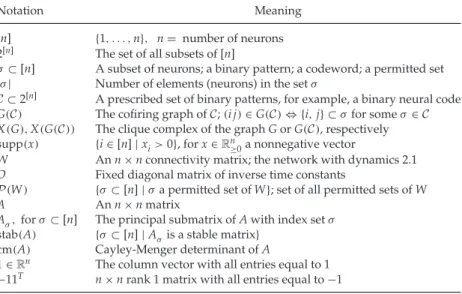
The organization of this letter is as follows. In section 2 we introduce some necessary background on binary neural codes, threshold-linear net-works, and permitted sets. In section 3, we introduce the encoding rule and present our results. The proofs of our main results are given in section 4 and use ideas from classical distance and convex geometry, such as Cayley-Menger determinants (Blumenthal, 1953), establishing a novel connection between these areas of mathematics and neural network theory. Section 5 contains the discussion. The appendixes follow. Table 1 provides frequently used notation in this letter.
2 Background
2.1 Binary Neural Codes. A binary pattern on n neurons is simply a string of 0s and 1s, with a 1 for each active neuron and a 0 denoting silence; equivalently, it is a subset of (active) neurons,
σ⊂ {1, . . . ,n} def= [n].
A binary neural code (aka a combinatorial neural code; Curto, Itskov, Morri-son, Roth, & Walker, 2013; Osborne, Palmer, Lisberger, & Bialek, 2008) is a collection of binary patternsC⊂2[n], where 2[n]denotes the set of all subsets
of [n].
Experimentally observed neural activity in cortical and hippocampal areas suggests that neural codes are sparse (Hrom´adka, Deweese, & Zador,
Table 1: Frequently Used Notation.
Notation Meaning
[n] {1, . . . ,n}, n= number of neurons 2[n] The set of all subsets of [n]
σ ⊂[n] A subset of neurons; a binary pattern; a codeword; a permitted set |σ| Number of elements (neurons) in the setσ
C⊂2[n] A prescribed set of binary patterns, for example, a binary neural code
G(C) The cofiring graph ofC;(i j)∈G(C)⇔ {i,j} ⊂σfor someσ∈C X(G),X(G(C)) The clique complex of the graph G or G(C), respectively supp(x) {i∈[n]|xi>0}, for x∈Rn
≥0a nonnegative vector
W An n×n connectivity matrix; the network with dynamics 2.1 D Fixed diagonal matrix of inverse time constants
P(W) {σ⊂[n]|σa permitted set of W}; set of all permitted sets of W
A An n×n matrix
Aσ,forσ⊂[n] The principal submatrix of A with index setσ stab(A) {σ⊂[n]|Aσis a stable matrix}
cm(A) Cayley-Menger determinant of A
1∈Rn The column vector with all entries equal to 1 −11T n×n rank 1 matrix with all entries equal to−1
2008; Barth & Poulet, 2012), meaning that relatively few neurons are coactive in response to any given stimulus. Correspondingly, we say that a binary neural codeC⊂2[n]is k-sparse, for k<n, if all patternsσ∈Csatisfy|σ| ≤k.
Note that in order for a codeC to have good error-correcting capability, the total number of code words|C|must be considerably smaller than 2n
(MacWilliams & Sloane, 1983; Huffman & Pless, 2003; Curto et al., 2013), a fact that may account for the limited repertoire of observed neural activity. Important examples of binary neural codes are classical population codes, such as receptive field codes (RF codes) (Curto et al., 2013). A sim-ple yet paradigmatic examsim-ple is the hippocampal place field code (PF code), where single neuron activity is characterized by place fields (O’Keefe, 1976; O’Keefe & Nadel, 1978). We consider general RF codes in section 3.6 and specialize to sparse PF codes in section 3.7.
2.2 Threshold-Linear Networks. A threshold-linear network (Hahnloser et al., 2003; Curto et al., 2012) is a firing rate model for a recurrent network (Dayan & Abbott, 2001; Ermentrout & Terman, 2010), where the neurons all have threshold nonlinearity,φ(z)=[z]+=max{z,0}. The dynamics are given by dxi dt = − 1 τixi+φ ⎛ ⎝n j=1 Wi jxj+ei−θi ⎞ ⎠, i=1, . . . ,n,
where n is the number of neurons, xi(t)is the firing rate of the ith neuron at time t, eiis the external input to the ith neuron, andθi>0 is its threshold.
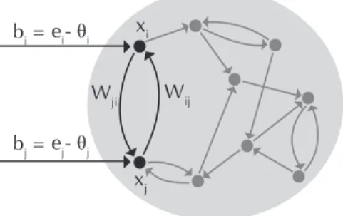
Figure 1: A recurrent network receiving an input vector b=(b1, . . . ,bn). The firing rate of each neuron is given by xi=xi(t)and evolves in time according to equation 2.1. The strengths of recurrent connections are captured by the matrix W.
The matrix entry Wijdenotes the effective strength of the connection from the jth to the ith neuron, and the timescaleτi>0 gives the rate at which a neuron’s activity decays to zero in the absence of any inputs (see Figure 1). Although sigmoids more closely match experimentally measured input-output curves for neurons, the above-threshold nonlinearity is often a good approximation when neurons are far from saturation (Dayan & Abbott, 2001; Shriki, Hansel, & Sompolinsky, 2003). Assuming that encoded pat-terns of a network are in fact realized by neurons that are firing far from saturation, it is reasonable to approximate them as stable fixed points of the threshold-linear dynamics.
These dynamics can be expressed more compactly as
˙
x= −Dx+[Wx+b]+, (2.1)
where Ddef= diag(1/τ1, . . . ,1/τn)is the diagonal matrix of inverse time con-stants, W is the synaptic connectivity matrix, b=(b1, . . . ,bn)∈Rn with
bi=ei−θi, and [·]+is applied elementwise. Note that unlike in the Hop-field model, the “input” to the network comes in the form of a constant (in time) external drive b rather than an initial condition x(0). We think of equation 2.1 as describing the fast-timescale dynamics of the network and b as representing the effect of an external stimulus. So long as b changes slowly as compared to the fast network dynamics, the neural responses to individual stimuli are captured by the steady states of equation 2.1 in the presence of a constant input vector b.
In the encoding rule (see section 3.1), we assume homogeneous timescales and use D=I (the identity matrix). Nevertheless, all results ap-ply equally well to heterogeneous timescales (i.e., for any diagonal D hav-ing strictly positive diagonal). We also assume that−D+W has a strictly
negative diagonal, so that the activity of an individual neuron always decays to zero in the absence of external or recurrent inputs. Although we consider responses to the full range of inputs b∈Rn, the possible steady states of
equation 2.1 are sharply constrained by the connectivity matrix W. Assum-ing fixed D, we refer to a particular threshold-linear network simply as W.
2.3 Permitted Sets of Threshold-Linear Networks. We consider threshold-linear networks whose computational function is to encode a set of binary patterns. These patterns are stored as “permitted sets” of the network. The theory of permitted (and forbidden) sets was introduced in Xie et al. (2002) and Hahnloser et al. (2003), and many interesting results were obtained in the case of symmetric threshold-linear networks. Here we review some definitions and results that apply more generally, though later we will also restrict ourselves to the symmetric case.
Informally, a permitted set of a recurrent network is a binary pattern σ⊂[n] that can be activated. This means there exists an external input to the network such that the neural activity x(t)=(x1(t), . . . ,xn(t))converges to a steady state x∗∈Rn
≥0(i.e., x∗is a stable fixed point with all firing rates
nonnegative) having supportσ: σ=supp(x∗) def= {i∈[n]|x∗i >0}.
Definition 1. A permitted set of the network 2.1 is a subset of neuronsσ ⊂[n] with the property that for at least one external input b∈Rn, there exists an
asymptotically stable fixed point x∗∈Rn
≥0 such that σ= supp(x∗) (Hahnloser
et al., 2003). For a given choice of network dynamics, the connectivity matrix W determines the set of all permitted sets of the network, denotedP(W).
For threshold-linear networks of the form 2.1, it has been previously shown that permitted sets of W correspond to stable principal submatrices of−D+W (Hahnloser et al., 2003; Curto et al., 2012). Recall that a stable matrix is one whose eigenvalues all have strictly negative real part. For any n×n matrix A, the notation Aσ denotes the principal submatrix obtained by restricting to the index setσ; ifσ= {s1, . . . ,sk}, then Aσ is the k×k matrix with(Aσ)i j=As
isj. We denote the set of all stable principal submatrices of A as
stab(A) def= {σ⊂[n]|Aσ is a stable matrix}.
With this notation we can now restate our prior result, which generalizes an earlier result of Hahnloser et al. (2003) to nonsymmetric networks.
Theorem 1(Curto et al., 2012, theorem 1.2).1 Let W be a threshold-linear network
on n neurons (not necessarily symmetric) with dynamics given by equation 2.1, and letP(W) be the set of all permitted sets of W. Then
P(W) = stab(−D + W).
Theorem 1 implies that a binary neural codeCcan be exactly encoded as the set of permitted sets in a threshold-linear network if and only if there exists a pair of n×n matrices(D,W) such thatC=stab(−D+W). From this observation, it is not difficult to see that not all codes are realizable by threshold-linear networks. This follows from a simple lemma:
Lemma 1. Let A be an n×n real-valued matrix (not necessarily symmetric) with strictly negative diagonal and n≥2. If A is stable, then there exists a 2×2 principal submatrix of A that is also stable.
Proof. We use the formula for the characteristic polynomial in terms of sums of principal minors:
pA(X)=(−1)nXn+(−1)n−1m1(A)Xn−1
+(−1)n−2m
2(A)Xn−2+ · · · +mn(A),
where mk(A)is the sum of the k×k principal minors of A. Writing the char-acteristic polynomial in terms of symmetric polynomials in the eigenvalues λ1, λ2, . . . , λn, and assuming A is stable, we have m2(A)=
i<jλiλj>0.
This implies that at least one 2×2 principal minor is positive. Since the cor-responding 2×2 principal submatrix has negative trace, it must be stable.
Combining lemma 1 with theorem 1 then gives:
Corollary 1. LetC⊂2[n]. If there exists a patternσ∈C such that no order 2
subset ofσ belongs toC, thenCis not realizable asC=P(W) for any threshold-linear network W.
Here we will not pay attention to the relationship between the input to the network b and the corresponding permitted sets that may be activated, as it is beyond the scope of this letter. In prior work, however, we were able to understand with significant detail the relationship between a given b and the set of resulting fixed points of the dynamics (Curto et al., 2012, proposition 2.1). For completeness, we summarize these findings in appendix D.
1Note that in Curto et al. (2012, theorem 1.2), permitted sets were called “stable sets.”
2.4 Structure of Permitted Sets of Symmetric Threshold-Linear Net-works. In the remainder of this work, we restrict attention to the case of symmetric networks. With this assumption, we can immediately say more about the structure of permitted setsP(W). Namely, if W is symmetric, then the permitted setsP(W)have the combinatorial structure of a simpli-cial complex.
Definition 2. An (abstract) simplicial complex Δ⊂2[n] is a set of subsets of
[n] ={1, . . . ,n} such that the following two properties hold: (1) for each i ∈ [n],{i} ∈Δ, and (2) ifσ ∈Δandτ ⊂σ, thenτ ∈Δ.
Lemma 2. If W is a symmetric threshold-linear network, thenP(W) is a simplicial complex.
In other words, if W is symmetric, then every subset of a permitted set is permitted, and every superset of a set that is not permitted is also not permitted. This was first observed in Hahnloser et al. (2003), using an ear-lier version of theorem 1 for symmetric W. It follows from the fact that
P(W)=stab(−D+W), by theorem 1, and stab(A)is a simplicial complex for any symmetric n×n matrix A having strictly negative diagonal (see corollary 7 in appendix A). The proof of this fact is a straightforward appli-cation of Cauchy’s interlacing theorem (appendix A), which applies only to symmetric matrices.
We are not currently aware of any simplicial complex that is not realizable as=P(W)for a symmetric threshold-linear network, although we believe such examples are likely to exist.
3 Results
Theorem 1 allows one to find all permitted setsP(W)of a given network W. Our primary interest, however, is in the inverse problem:
NE problem: Given a set of binary patternsC⊂2[n], how can one construct
a network W such that C⊆P(W), while minimizing the emergence of unwanted spurious states?
Note that spurious states are elements ofP(W)that were not in the pre-scribed set of patterns to be stored; these are precisely the elements of
P(W)\C. IfC⊂P(W), so that all patterns inCare stored as permitted sets of W butP(W)may contain additional spurious states, then we say that
C has been encoded by the network W. If C=P(W), so that there are no spurious states, then we say thatChas been exactly encoded by W.
We tackle the NE problem by analyzing a novel learning rule, called the encoding rule. In what follows, the problem is broken into four motivating questions that address (1) the learning rule, (2) the resulting structure of permitted sets, (3) binary codes that are exactly encodable, and (4) the
structure of spurious states when codes are not encoded exactly. In section 3.6 we use our results to uncover “natural” codes for symmetric threshold-linear networks and illustrate this phenomenon in the case of hippocampal PF codes in section 3.7.
3.1 The Encoding Rule
Question 1: Is there a biologically plausible learning rule that allows arbitrary neural codes to be stored as permitted sets in threshold-linear networks?
In this section we introduce a novel encoding rule that constructs a network W from a prescribed set of binary patternsC. The rule is similar to the classical Hopfield learning rule (Hopfield, 1982) in that it updates the weights of the connectivity matrix W following sequential presentation of binary patterns, and strengthens excitatory synapses between coactive neurons in the patterns. In particular, the rule is Hebbian and local: each synapse is updated only in response to the coactivation of the two adja-cent neurons, and the updates can be implemented by presenting only one pattern at a time (Hopfield, 1982; Dayan & Abbott, 2001). A key difference from the Hopfield rule is that the synapses are binary: once a synapse(i j) has been turned “on,” the value of Wijstays the same irrespective of the remaining patterns.2 A new ingredient is that synapses are allowed to be
heterogeneous: in other words, the actual weights of connections are varied among “on” synapses. These weights are assigned according to a predeter-mined synaptic strength matrix S, which is considered fixed and reflects the underlying architecture of the network. For example, if no physical connec-tion exists between neurons i and j, then Si j=0, indicating that no amount of cofiring can cause a direct excitatory connection betwen those neurons. On the other hand, if two neurons have multiple points of physical contact, then Sij will be greater than if there are only a few anatomical contacts. There is, in fact, experimental evidence in hippocampus for synapses that appear binary and heterogeneous in this sense (Petersen, Malenka, Nicoll, & Hopfield, 1998), with individual synapses exhibiting potentiation in an all-or-nothing fashion, but having different thresholds for potentiation and heterogeneous synaptic strengths.
Here we describe the encoding rule in general, with minimal assump-tions on S. Later, in secassump-tions 3.4 and 3.5, we investigate the consequences of various choices of S on the network’s ability to encode different types of binary neural codes.
Encoding rule. This is a prescription for constructing (i.e., “learning”) a network W from a set of binary patterns on n neurons,C⊂2[n] (e.g.,C is
a binary neural code). It consists of three steps: two initialization steps, followed by an update step:
Step 1: Fix an n×n synaptic strength matrix S and anε >0. We think of S andεas intrinsic properties of the underlying network architecture, established prior to learning. Because S contains synaptic strengths for symmetric excitatory connections, we require that Si j=Sji≥0 and Sii=0.
Step 2: The network W is initialized to be symmetric with effective con-nection strengths Wi j=Wji<−1 for i= j, and Wii=0. (Beyond this requirement, the initial values of W do not affect the results.) Step 3: Following presentation of each patternσ∈C, we turn “on” all
excitatory synapses between neurons that coappear inσ.3This means
we update the relevant entries of W as follows: Wi j:= −1+εSi j if i,j∈σand i= j.
Note that the order of presentation does not matter; once an excitatory connection has been turned “on,” the value of Wij stays the same irrespective of remaining patterns.
To better understand what kinds of networks result from the encoding rule, observe that any initial W in step 2 can be written as Wi j= −1−εRi j, where Ri j=Rji>0 for i= j and Rii= −1/ε, so that Wii=0. Assuming a threshold-linear network with homogeneous timescales (i.e., fixing D=I), the final network W obtained fromCafter step 3 satisfies
(−D+W)i j= ⎧ ⎪ ⎨ ⎪ ⎩ −1+εSi j, if(i j)∈G(C) −1, if i= j −1−εRi j if(i j) /∈G(C), (3.1)
where G(C)is the graph on n vertices (neurons) having an edge for each pair of neurons that coappears in one or more patterns ofC. We call this graph the cofiring graph ofC. In essence, the rule allows the network to “learn” G(C), selecting which excitatory synapses are turned “on” and assigned to their predetermined weights.
3By presentation of each pattern, we mean that patterns are considered one at a time
in building the W matrix, without regard to the dynamics of equation 2.1 (see Hopfield, 1982; Xie et al., 2002).
Consequently, any matrix−D+W obtained via the encoding rule has the form
−11T+εA,
where−11Tdenotes the n×n matrix of all−1s and A is a symmetric matrix
with zero diagonal and off-diagonal entries Ai j=Si j≥0 or Ai j= −Ri j<0, depending onC. It then follows from theorem 1 that the permitted sets of this network are
P(W)=stab(−11T+εA).
Furthermore, it turns out thatP(W)for any symmetric W is of this form, even if−D+W is not of the form−11T+εA.
Lemma 3. If W is a symmetric threshold-linear network (with D not necessarily equal to the identity matrix I), then there exists a symmetric n×n matrix A with zero diagonal such thatP(W) = stab(−11T+ A).
The proof is given in appendix B (see lemma 14).
In addition to being symmetric, the encoding rule (for small enough ε) generates “lateral inhibition” networks where the matrix −D+W has strictly negative entries. In particular, this means that the matrix D−W is copositive—that is, xT(D−W)x>0 for all nonnegative x except x=0. It
fol-lows from (Hahnloser et al., 2003, theorem 1) that for all input vectors b∈Rn
and for all initial conditions, the network dynamics of equation 2.1 converge to an equilibrium point. This was proven by constructing a Lyapunov-like function, similar to the strategy in Cohen and Grossberg (1983).4
3.2 Main Result
Question 2: What is the full set of permitted setsP(W)stored in a network constructed using the encoding rule?
Our main result, theorem 2, characterizes the full set of permitted sets
P(W)obtained using the encoding rule, revealing a detailed understand-ing of the structure of spurious states. Recall from lemma 3 that the set of permitted sets of any symmetric network on n neurons has the form
P(W)=stab(−11T+εA),forε >0 and A a symmetric n×n matrix with
zero diagonal.5DescribingP(W)thus requires understanding the stability
4Note that threshold-linear networks do not directly fall into the very general class of
networks discussed in Cohen and Grossberg (1983).
5In fact, anyP(W)of this form can be obtained by perturbing around any rank 1
matrix—not necessarily symmetric—having strictly negative diagonal (proposition 3 in appendix B).
of the principal submatrices(−11T+εA)
σfor eachσ⊂[n]. Note that these submatrices all have the same form: −11T+εA
σ, where −11T is the all
−1s matrix of size|σ| × |σ|. Proposition 1 (below) provides an unexpected connection between the stability of these matrices and classical distance geometry.6We first present proposition 1 and then show how it leads to
theorem 2.
For symmetric 2×2 matrices of the form −11T+εA=
−1 −1+εA
12
−1+εA12 −1
, with ε >0, it is easy to identify the condi-tions for the matrix to be stable. One needs the determinant to be positive, so A12>0 and ε <2/A12. For 3×3 matrices, the conditions are more interesting, and the connection to distance geometry emerges.
Lemma 4. Consider the 3×3 matrix−11T+εA, for a fixed symmetric A with
zero diagonal: ⎡ ⎢ ⎣ −1 −1 +εA12 −1 +εA13 −1 +εA12 −1 −1 +εA23 −1 +εA13 −1 +εA23 −1 ⎤ ⎥ ⎦.
There exists anε >0 such that this matrix is stable if and only ifA12,A13, andA23are valid edge lengths for a nondegenerate triangle inR2.
In other words, the numbersAi jmust satisfy the triangle inequalities
Ai j<Aik+Ajk for distinct i,j,k. This can be proven by straightfor-ward computation, using Heron’s formula and the characteristic polyno-mial of the matrix. The upper bound onε, however, is not so easy to identify. Remarkably, the above observations completely generalize to n×n ma-trices of the form−11T+εA, and the precise limits onεcan also be
com-puted for general n. This is the content of proposition 1, below. To state it, however, we first need a few notions from distance geometry.
Definition 3. An n×n matrix A is a (Euclidean) square distance matrix if there exists a configuration of points p1, . . . ,pn∈Rn−1(not necessarily distinct) such
that Ai j =pi−pj2. A is a nondegenerate square distance matrix if the
corre-sponding points are affinely independent, that is, if the convex hull of p1, . . . ,pn is a simplex with nonzero volume inRn−1.
Clearly, all square distance matrices are symmetric and have zero diagonal. Furthermore, a 2×2 matrix A is a nondegenerate square distance matrix if
6Distance geometry is a field of mathematics that was developed in the early twentieth
century, motivated by the following problem: find necessary and sufficient conditions such that a finite set of distances can be realized from a configuration of points in Euclidean space. The classic text on this subject is Blumenthal (1953).
and only if the off-diagonal entry satisfies the additional condition A12>0. For a 3×3 matrix A, the necessary and sufficient condition to be a nonde-generate square distance matrix is that the entriesA12,A13,andA23 are valid edge lengths for a nondegenerate triangle inR2(this was precisely
the condition in lemma 4). For larger matrices, however, the conditions are less intuitive. A key object for determining whether an n×n matrix A is a nondegenerate square distance matrix is the Cayley-Menger determinant,
cm(A) def= det 0 1T 1 A ,
where 1∈Rnis the column vector of all ones. If A is a square distance
matrix, then cm(A) is proportional to the square volume of the simplex obtained as the convex hull of the points{pi}(see lemma 11 in appendix A). In particular, cm(A)=0 (and hence|cm(A)|>0) if A is a nondegenerate square distance matrix, while cm(A)=0 for any other (degenerate) square distance matrix.
Proposition 1. Let A be a symmetric n×n matrix with zero diagonal andε >0. Then the matrix
−11T+εA
is stable if and only if the following two conditions hold: (a) A is a nondegenerate square distance matrix, and (b) 0< ε <|cm(A)/det(A)|.
Proposition 1 is essentially a special case of theorem 4—our core technical result—whose statement and proof are given in section 4.1. The proof of proposition 1 is then given in section 4.2. To our knowledge, theorem 4 is novel, and connections to distance geometry have not previously been used in the study of neural networks or, more generally, the stability of fixed points in systems of ODEs.
The ratio|cm(A)/det(A)|has a simple geometric interpretation in cases where condition (a) of proposition 1 holds. Namely, if A is an n×n nonde-generate square distance matrix (with n>1), then|cm(A)/det(A)| = 1
2ρ2,
where ρ is the radius of the unique sphere circumscribed on any set of points in Euclidean space that can be used to generate A (see remark 6 in appendix C). Moreover, since|cm(A)|>0 whenever A is a nondegenerate square distance matrix, there always exists anεsmall enough to satisfy the second condition, provided the first condition holds. Combining proposi-tion 1 with Cauchy’s interlacing theorem yields:
Lemma 5. If A is an n×n nondegenerate square distance matrix, then 0<cm(Aσ) det(Aσ) ≤cm(Aτ) det(Aτ) if τ ⊆σ⊆[n].
Given any symmetric n×n matrix A with zero diagonal andε >0, it is now natural to define the following simplicial complexes:
geomε(A) def=
σ⊆[n]|Aσ a nondeg. sq. dist. matrix and
cm(Aσ) det(Aσ) > ε , and
geom(A) def= lim
ε→0geomε(A)={σ⊆[n]|Aσ a nondeg. sq. dist. matrix}.
Lemma 5 implies that geomε(A)and geom(A)are simplicial complexes. Note that ifσ = {i}, we have Aσ =[0]. In this case,{i} ∈geom(A)and{i} ∈ geomε(A)for allε >0 by our convention. Also, geomε(A)=geom(A)if and only if 0< ε < δ(A), where
δ(A) def= mincm(Aσ) det(Aσ) σ∈geom(A) .
If A is a nondegenerate square distance matrix, thenδ(A)=|cm(A)/det(A)|. To state our main result, theorem 2, we also need a few standard notions from graph theory. A clique in a graph G is a subset of vertices that is all-to-all connected.7The clique complex of G, denoted X(G), is the set of all cliques
in G; this is a simplicial complex for any G. Here we are primarily interested in the graph G(C), the cofiring graph of a set of binary patternsC⊂2[n].
Theorem 2. Let S be an n×n synaptic strength matrix satisfying Si j= Sji ≥0 and Sii = 0 for all i,j∈[n], and fix ε >0. Given a set of prescribed patterns
C⊂2[n], let W be the threshold-linear network (see equation 3.1) obtained fromC
using S andεin the encoding rule. Then,
P(W) = geomε(S)∩X(G(C)).
If we further assume thatε < δ(S), thenP(W) = geom(S)∩X(G(C)).
7For recent work encoding cliques in Hopfield networks, see Hillar, Tran, and Koepsell
In other words, a binary patternσ⊂[n] is a permitted set of W if and only if Sσ is a nondegenerate square distance matrix,ε <|cm(Sσ)/det(Sσ)|, andσ is a clique in the graph G(C).
The proof is given in section 4.2. Theorem 2 answers question 2 and makes explicit howP(W)depends on S,ε, andC. One way of interpreting this result is to observe that a binary patternσ∈Cis successfully stored as a permitted set of W if and only if the excitatory connections between the neurons inσ, given byS˜σ =εSσ, are geometrically balanced:
r
S˜σ is a nondegenerate square distance matrix.r
|det(S˜σ)|<|cm(S˜σ)|.The first condition ensures a certain balance among the relative strengths of excitatory connections in the cliqueσ, while the second condition bounds the overall excitation strengths relative to inhibition (which has been nor-malized to−1 in the encoding rule).
We next turn to an example that illustrates how this theorem can be used to solve the NE problem explicitly for a small binary neural code. In the following section, section 3.4, we address more generally the question of what neural codes can be encoded exactly and what the structure of spurious states is when a code is encoded inexactly.
3.3 An Example. SupposeC is a binary neural code on n=6 neurons, consisting of maximal patterns
{110100,101010,011001,000111},
corresponding to subsets {124},{135},{236},and {456}, together with all subpatterns (smaller subsets) of the maximal ones, thus ensuring thatCis a simplicial complex. This is depicted in Figure 2A, using a standard method of illustrating simplicial complexes geometrically. The four maximal pat-terns correspond to the shaded triangles, while patpat-terns with only one or two coactive neurons comprise the vertices and edges of the cofiring graph G(C).8
Without theorem 2, it is difficult to find a network W that encodesC exactly—that is, such thatP(W)=C. This is in part because each connec-tion strength Wijbelongs to two 3×3 matrices that must satisfy opposite stability properties. For example, subset{124}must be a permitted set of
P(W), while{123}is not permitted, imposing competing conditions on the entry W12. In general, it may be difficult to patch together local ad hoc solu-tions to obtain a single matrix W having all the desired stability properties.
8In this example, there are no patterns having four or more neurons, but these would
Figur e 2: An example on n = 6 n eur ons. (A) The simplicial complex C consists of 4 two-dimensional facets (shaded triangles). T he graph G ( C ) contains the 6 v ertices and 12 depicted edges; these ar e also included in C , so the size of the code is | C |= 22. (B) A configuration of points p1 ,..., p6 ∈ R 2that can be used to exactly encode C .L ines indicate triples o f p oints that ar e collinear .Fr om this configuration, we constr uct a 6 × 6 synaptic str ength m atrix S , with Sij = pi − pj 2, and choose 0 <ε <δ ( S ) .T h e g eo m et ry of the configuration implies that geom ( S ) does not contain any p atterns o f size gr eater than 3 or the triples { 123 } , { 145 } , { 246 } , or { 356 } . It is straightforwar d to check that C = geom ( S ) ∩ X ( G ( C )) . (C) Another solution for exactly encoding C is pr ovided by choosing the matrix S with Sij given b y the labeled edges in the figur e. The squar e d istances in Sij wer e chosen to satisfy the triangle inequalities for shaded triangles but to violoate them for empty triangles.
Using theorem 2, however, we can easily construct many exact solutions for encodingCas a set of permitted setsP(W). The main idea is as follows. Consider the encoding rule with synaptic strength matrix S and 0< ε < δ(S). Applying the rule toCyields a network with permitted sets
P(W)=geom(S)∩X(G(C)).
The goal is thus to find S so thatC=geom(S)∩X(G(C)).From the cofiring graph G(C), we see that the clique complex X(G(C)) contains all trian-gles depicted in Figure 2A, including the empty (nonshaded) triantrian-gles:
{123},{145},{246},and {356}. The matrix S must therefore be chosen so that these triples are not in geom(S), while ensuring that{124},{135},{236}, and {456} are included. In other words, to obtain an exact solution, we must find S such that Sσ is a nondegenerate square distance matrix for eachσ ∈ {{124},{135},{236},{456}}but not forσcorresponding to an empty triangle.
Solution 1. Consider the configuration of points p1, . . . ,p6∈R2in
Fig-ure 2B, and let S be the 6×6 square distance matrix with entries Si j=
pi−pj2. Because the points lie in the plane, the largest principal
sub-matrices of S that can possibly be nondegenerate square distance sub-matrices are 3×3. This means geom(S)has no elements of size greater than 3. Be-cause no two points have the same position, geom(S)contains the complete graph with all edges(i j). It remains only to determine which triples are in geom(S). The only 3×3 principal submatrices of S that are nondegen-erate square distance matrices correspond to triples of points in general position. From Figure 2B (left), we see that geom(S) includes all triples except {123},{145},{246},and {356}, since these correspond to triples of points that are collinear (and thus yield degenerate square distance matri-ces). AlthoughC=X(G(C))andC=geom(S), it is now easy to check that
C=geom(S)∩X(G(C)). Using theorem 2, we conclude thatC=P(W) ex-actly, where W is the network obtained using the encoding rule with this S and any 0< ε < δ(S).
Solution 2. Let S be the symmetric matrix defined by the following equations for i< j: Si j=1 if i=1; S24=S35=1; S23=S26=S36=32; and
Si j=52 if i = 4 or 5. Here we have only assigned values
correspond-ing to each edge in G(C)(see Figure 2C); remaining entries may be cho-sen arbitrarily, as they play no role after we intersect geom(S)∩X(G(C)). Note that S is not a square distance matrix at all, not even a degener-ate one. Nevertheless, Sσ is a nondegenerate square distance matrix for σ ∈ {{124},{135},{236},{456}}, because the distances correspond to non-degenerate triangles. For example, the triple{124}has pairwise distances (1,1,1), which satisfy the triangle inequality. In contrast, the triple{123}has pairwise distances (1,1,3), which violate the triangle inequality; hence, S{123}is not a square distance matrix. Similarly, the triangle inequality is
violated for each of{145},{246},and{356}. It is straightforward to check that among all cliques of X(G(C)), only the desired patterns inC are also elements of geom(S), soC=geom(S)∩X(G(C)).
By construction, solutions 1 and 2 produce networks W (obtained using the encoding rule withε,S, andC) with exactly the same set of permitted sets P(W). Nevertheless, the solutions are functionally different in that the resulting input-output relationships associated with the equation 2.1 dynamics are different, as they depend on further details of W not captured byP(W)(see appendix D).
3.4 Binary Neural Codes That Can Be Encoded Exactly
Question 3: What binary neural codes can be encoded exactly asC=P(W) for a symmetric threshold-linear network W?
Question 4: If encoding is not exact, what is the structure of spurious states? From theorem 2, it is clear that if the set of patterns to be encoded happens to be of the formC=geom(S)∩X(G(C)), thenC can be exactly encoded asP(W)for small enoughεand the same choice of S. Similarly, if the set of patterns has the formC=geomε(S)∩X(G(C)), thenCcan be exactly encoded asP(W)using our encoding rule (see section 3.1) with the same S andε. Can any other sets of binary patterns be encoded exactly via symmetric threshold-linear networks? The next theorem assures us that the answer is no. This means that by focusing attention on networks constructed using our encoding rule, we are not missing any binary neural codes that could arise asP(W)for other symmetric networks.
Theorem 3. LetC⊂2[n] be a binary neural code. There exists a symmetric
threshold-linear network W such thatC=P(W) if and only ifC is a simplicial complex of the form
C= geomε(S)∩X(G(C)), (3.2)
for someε >0 and S an n×n matrix satisfying Si j = Sji ≥0 and Sii = 0 for all i,j∈[n]. Moreover, W can be constructed using the encoding rule onC, using this choice of S andε.
The proof is given in section 4.2. Theorem 3 allows us to make a preliminary classification of binary neural codes that can be encoded exactly, giving a
partial answer to question 3. To do this, it is useful to distinguish three different types of S matrices that can be used in the encoding rule:
r
Universal S. We say that a matrix S is universal if it is an n×nnondegenerate square distance matrix. In particular, any principal submatrix Sσ is also a nondegenerate square distance matrix, so if we let 0< ε < δ(S)=cm(S)/det(S), then anyσ∈C has corre-sponding excitatory connectionsεSσthat are geometrically balanced (see section 3.2). Furthermore, geomε(S)=geom(S)=2[n], and hence
geomε(S)∩X(G(C))=X(G(C)), irrespective of S. It follows that if
C=X(G)for any graph G, thenCcan be exactly encoded using any universal S and any 0< ε < δ(S) in the encoding rule.9 Moreover,
sinceC⊂X(G(C)) for any codeC, it follows that any code can be encoded—albeit inexactly—using a universal S in the encoding rule. Finally, the spurious statesP(W)\Ccan be completely understood: they consist of all cliques in the graph G(C)that are not elements of
C.
r
k-sparse universal S. We say that a matrix S is k-sparse universal if itis a (degenerate) n×n square distance matrix for a configuration of n points that are in general position10inRk−1,for k<n (otherwise S is
universal). Let 0< ε < δ(S). Then, geomε(S)=geom(S)= {σ⊂[n]|
|σ| ≤k}; this is the(k−1)–skeleton11of the complete simplicial
com-plex 2[n]. This implies that geom
ε(S)∩X(G(C))=Xk−1(G(C)), where
Xkdenotes the k-skeleton of the clique complex X: Xk(G(C)) def= {σ∈X(G(C))| |σ| ≤k+1}.
It follows that any k-skeleton of a clique complex,C=Xk(G)for any graph G, can be encoded exactly. Furthermore, since any k-sparse codeC satisfiesC⊆Xk−1(G(C)), any k-sparse code can be encoded using this type of S matrix in the encoding rule. The spurious states in this case are cliques of G(C)that have size no greater than k.
r
Specially tuned S. We will refer to all S matrices that do not fall intothe universal or k-sparse universal categories as specially tuned. In this case, we cannot say anything general about the codes that are exactly encodable without further knowledge about S. If we let 0< ε < δ(S), as above, theorem 3 tells us that the binary codes C
that can be encoded exactly (via the encoding rule) are of the form
9Note that ifC=X(G)is any clique complex with underlying graph G, then we
automatically know that G(C)=G, and hence X(G(C))=X(G)=C.
10This guarantees that all k×k principal submatrices of S are nondegenerate square
distance matrices.
11The k-skeleton
kof a simplicial complexis obtained by restricting to faces of dimension≤k, which corresponds to keeping only elementsσ⊂of size|σ| ≤k+1. Note thatkis also a simplicial complex.
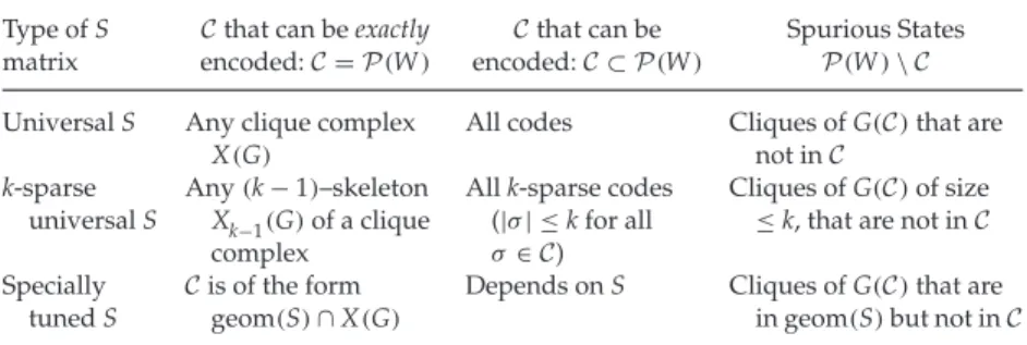
Table 2: Classification of S Matrices, Together with Encodable Codes and Spu-rious States.
Type of S matrix
Cthat can be exactly encoded:C=P(W)
Cthat can be encoded:C⊂P(W)
Spurious States P(W)\C Universal S Any clique complex
X(G)
All codes Cliques of G(C)that are not inC k-sparse universal S Any(k−1)–skeleton Xk−1(G)of a clique complex
All k-sparse codes (|σ| ≤k for all
σ∈C)
Cliques of G(C)of size ≤k, that are not inC Specially
tuned S
Cis of the form geom(S)∩X(G)
Depends on S Cliques of G(C)that are in geom(S)but not inC Notes: The above assumes using the encoding rule on the codeCwith synaptic strength matrix S and 0< ε < δ(S). Additional codes may be exactly encodable for other choices ofε.
C=geom(S)∩X(G(C)). Unlike in the universal and k-sparse univer-sal cases, the encodable codes depend on the precise form of S. Note that the example codeC discussed in section 3.3 was not a clique complex or the k-skeleton of a clique complex. Nevertheless, it could be encoded exactly for the “specially tuned” choices of S exhibited in solutions 1 and 2 (see Figures 2B and 2C).
A summary of what codes are encodable and exactly encodable for each type of S matrix is shown in Table 2, under the assumption that 0< ε < δ(S) in the encoding rule.
We end this section with several technical remarks, along with some open questions for further mathematical investigation.
Remark 1. Fine-tuning? It is worth noting here that solutions obtained by choosing S to be a degenerate square distance matrix, as in the k-sparse uni-versal S or the specially tuned S of Figure 2B, are not as finely tuned as they might first appear. This is because the ratio|cm(Sσ)/det(Sσ)|approaches zero as subsets of points{pi}i∈σ used to generate S become approximately degenerate, allowing elements to be eliminated from geomε(S)because of violations to condition (b) in proposition 1, even if condition (a) is not quite violated. This means the appropriate matrices do not have to be exactly de-generate, but only approximately degenerate (see remark 7 in appendix C). In particular, the collinear points in Figure 2B need not be exactly collinear for solution 1 to hold.
Remark 2. Controlling spurious cliques in sparse codes. If the set of patterns
C⊂2[n]to be encoded is a k-sparse code, that is, if|σ| ≤k<n for allσ∈C,
then any clique of size k+1 or greater in G(C) is potentially a spurious clique. We can eliminate these spurious states, however, by choosing a k-sparse universal S in the encoding rule. This guarantees that geomε(S)
does not include any element of size greater than k, and hence P(W)⊆ Xk−1(G(C)).
Remark 3. Uniform S. To use truly binary synapses, we can choose S in the encoding rule to be the uniform synaptic strength matrix having Si j=1 for i= j and Sii=0 for all i∈[n]. In fact, S is a nondegenerate square distance matrix, so this is a special case of a “universal” S. Hereδ(S)turns out to have a very simple form:
δ(S)=cm(S) det(S)
= n
n−1.
Similarly, any k×k principal submatrix Sσ, with|σ| =k, satisfiesδ(Sσ)=
k
k−1.This implies that geomε(S)is the k-skeleton of the complete simplicial complex on n vertices if and only if
k+2 k+1< ε <
k+1 k .
It follows that for this choice of S andε(note thatε > δ(S)), the encoding rule yieldsP(W)=Xk(G(C)), just as in the case of k-sparse universal S. If, on the other hand, we choose 0< ε≤1< δ(S), then geomε(S)=geom(S)=2[n],
and we have the usual properties for universal S.
Remark 4. Matroid complexes. In the special case where S is a square dis-tance matrix, geom(S)is a representable matroid complex—the independent set complex of a real-representable matroid (Oxley, 2011). Moreover, all representable matroid complexes are of this form and can thus be encoded exactly. To see this, take any codeChaving G(C)=Kn, the complete graph on n vertices. Then X(G(C))=2[n], and the encoding rule (for ε < δ(S))
yields
P(W)=geom(S).
Note that although the example code C of section 3.3 is not a matroid complex (in particular, it violates the independent set exchange property; Oxley, 2011), geom(S)for the matrix S given in solution 1 (see Figure 2B) is a representable matroid complex, showing thatCis the intersection of a representable matroid complex and the clique complex X(G(C)).
Remark 5. Open questions. Can a combinatorial description be found for all simplicial complexes that are of the form geomε(S)or geom(S), where S andεsatisfy the conditions in theorem 3? For such complexes, can the appropriate S andεbe obtained constructively? Does every simplicial com-plexCadmit an exact solution to the NE problem via a symmetric network
W? That is, is every simplicial complex of the form geomε(S)∩X(G(C)), as in equation 3.2? If not, what are the obstructions? More generally, does every simplicial complex admit an exact solution (not necessarily sym-metric) to the NE problem? We have seen that all matroid complexes for representable matroids can be exactly encoded as geom(S). Can nonrepre-sentable matroids also be exactly encoded?
3.5 Spurious States and “Natural” Codes. Although it may be possi-ble, as in the example of Section 3.3, to precisely tune the synaptic strength matrix S to exactly encode a particular neural code, this is somewhat con-trary to the spirit of the encoding rule, which assumes S to be an intrinsic property of the underlying network. Fortunately, as seen in section 3.4, theorem 2 implies that certain “universal” choices of S enable anyC⊂2[n]
to be encoded. The price to pay, however, is the emergence of spurious states.
Recall that spurious states are permitted sets that arise inP(W) that were not in the prescribed listCof binary patterns to be encoded. Theorem 2 immediately implies that all spurious states lie in X(G(C))—that is, every spurious state is a clique of the cofiring graph G(C). We can divide them into two types:
r
Type 1: Spurious subsets.These are permitted setsσ∈P(W)\Cthatare subsets of patterns inC. Note that ifCis a simplicial complex, there will not be any spurious states of this type. But ifCis not a simplicial complex, then type 1 spurious states are guaranteed to be present for any symmetric encoding rule, becauseP(W)=stab(−D+W)is a simplicial complex for symmetric W (see lemma 2).
r
Type 2: Spurious cliques.These are permitted setsσ∈P(W)\Cthat are not of the first type. Note that technically, the type 1 spurious states are also cliques in G(C), but we will use the term spurious clique to refer only to spurious states that are not spurious subsets.Perhaps surprisingly, some common neural codes have the property that the full set of patterns to be encoded naturally contains a large fraction of the cliques in the code’s cofiring graph. In such cases, C≈X(G(C)), or
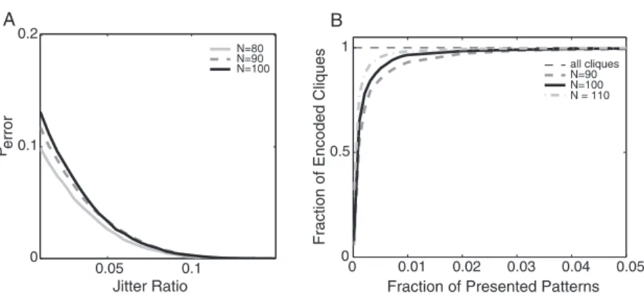
C≈Xk(G(C)). These neural codes therefore have very few spurious states when encoded using a universal or k-sparse universal S, even though S has not been specially tuned for the given code. We will refer to these as natural codes for symmetric threshold-linear networks because they have two im-portant properties that make them particularly fitting for these networks:
P1. Natural codes can be encoded exactly or nearly exactly, using any universal or k-sparse universal matrix S in the encoding rule. P2. Natural codes can be fully encoded following presentation of only
In other words, not only can natural codes be generically encoded with very few spurious states, but they can also be encoded from a highly undersampled set of codewords. This is because the network naturally fills in the missing elements via spurious states that emerge after encoding only part of the code. In the next two sections, we explain why RF codes are “natural” in this sense, and illustrate the above two properties with a concrete application of encoding two-dimensional PF codes, an important example of RF codes.
3.6 Receptive Field Codes Are Natural Codes. RF codes are binary neural codes consisting of activity patterns of populations of neurons that fire according to receptive fields.12 Abstractly, a receptive field is a map f
i:
S→R≥0from a space of stimuliSto the average firing rate fi(s)of a single
neuron i in response to each stimulus s∈S. Receptive fields are computed from experimental data by correlating neural responses to external stimuli. We follow a common abuse of language, where both the map and its support (i.e., the subset Ui⊂Swhere fitakes on strictly positive values) are referred to as receptive fields. If the stimulus space is d-dimensional,S⊂Rd, we say
that the receptive fields have dimension d. The paradigmatic examples of neurons with receptive fields are orientation-selective neurons in visual cortex (Ben-Yishai, Bar-Or, & Sompolinsky, 1995) and hippocampal place cells (McNaughton, Battaglia, Jensen, Moser, & Moser, 2006). Orientation-selective neurons have tuning curves that reflect a neuron’s preference for a particular angle. Place cells are neurons that have place fields (O’Keefe, 1976; O’Keefe & Nadel, 1978); that is, each neuron has a preferred (convex) region of the animal’s physical environment where it has a high firing rate. Both tuning curves and place fields are examples of low-dimensional receptive fields, having typical dimension d=1 or d=2.
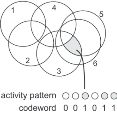
The elements of an RF code C correspond to subsets of neurons that may be coactivated in response to a stimulus s∈Rd (see Figure 3). Here
we define two variations of this notion, which we refer to as RF codes and coarse RF codes.
Definition 4. Let{U1, . . . ,Un}be a collection of convex open sets inRd, where
each Ui is the receptive field corresponding to the ith neuron. To such a set of
receptive fields, we associate a d-dimensional RF codeC, defined as follows: for each σ ∈2[n], σ∈C if and only if i∈σ Ui j∈/σ Uj=∅.
12In the vision literature, the term “receptive field” is reserved for subsets of the visual
1 4 2 3 5 0 0 1 0 1 1 codeword activity pattern 6
Figure 3: Two-dimensional receptive fields for six neurons. The RF codeChas a codeword for each overlap region. For example, the shaded region corresponds to the binary pattern 001011; equivalently, we denote it asσ= {3,5,6} ∈C. The corresponding coarse RF code also includes all subsets, such asτ= {3,5},even if they are not part of the original RF code.
This definition was previously introduced in Curto et al. (2013) and Curto, Itskov, Veliz-Cuba, and Youngs (in press). A coarse RF code is obtained from an RF code by including all subsets of code words, so that for eachσ ∈2[n],
σ∈C if and only if
i∈σ Ui= ∅.
Note that the codewordσ= {3,5,6}in Figure 3 corresponds to stimuli in the shaded region, not to the full intersection U3∩U5∩U6. Moreover, the subsetτ = {3,5} ⊂σis not an element of the RF code, since U3∩U5⊂ U6. Nevertheless, it often makes sense to also consider such subsets as codewords; for example, the cofiring of neurons 3 and 5 may still be ob-served, as neuron 6 may fail to fire even if the stimulus is in its receptive field. This is captured by the corresponding coarse RF code.
Coarse RF codes carry less detailed information about the underlying stimulus space (Curto & Itskov, 2008; Curto et al., in press), but turn out to be more “natural” in the context of symmetric threshold-linear networks because they have the structure of a simplicial complex.13 This implies
that coarse RF codes do not yield any type 1 spurious states—the spurious subsets—when encoded in a network using the encoding rule. Furthermore, both RF codes and coarse RF codes with low-dimensional receptive fields
13In topology, this simplicial complex is called the nerve of the cover{U
1, . . . ,Un}(see Bott & Tu, 1982; Curto & Itskov, 2008).
contain surprisingly few type 2 spurious states—the spurious cliques. This follows from Helly’s theorem, a classical theorem in convex geometry:
Helly’s theorem(Barvinok, 2002). Suppose that U1, . . . ,Ukis a finite collection of convex subsets ofRd, for d<k. If the intersection of any d+1 of these sets is
nonempty, then the full intersectionki=1Uiis also nonempty.
To see the implications of Helly’s theorem for RF codes, we define the notion of Helly completion:
Definition 5. LetΔdbe a d-dimensional simplicial complex on n vertices. The Helly completion ¯Δdis the largest simplicial complex on n vertices that hasΔdas its d-skeleton.
In other words, the Helly completion of a d-dimensional simplicial complex d is obtained by adding in all higher-dimensional faces in a way that is consistent with the existing lower-dimensional faces. In particular, the Helly completion of any graph G is the clique complex X(G). For a two-dimensional simplicial complex,2, the Helly completion includes only cliques of the underlying graph G(2) that are consistent with2. For example, the Helly completion of the code in section 3.3 does not include the 3-cliques corresponding to empty (nonshaded) triangles in Figure 2A. With this notion, Helly’s theorem can now be reformulated:
Lemma 6. LetC be a coarse d-dimensional RF code, corresponding to a set of place fields{U1, . . . ,Un}where each Uiis a convex open set inRd. ThenCis the
Helly completion of its own d-skeleton:C= ¯Cd.
This lemma indicates that low-dimensional RF codes, whether coarse or not, have a relatively small number of spurious cliques, since most cliques in X(G(C))are also in the Helly completionC¯dfor small d. In particular, it
implies that coarse RF codes of dimensions d=1 and d=2 are very natural codes for symmetric threshold-linear networks.
Corollary 2. IfCis a coarse one-dimensional RF code, then it is a clique complex:
C= ¯C1= X(G(C)). Therefore,C can be exactly encoded using any universal S in
the encoding rule.
Corollary 3. If C is a coarse two-dimensional RF code, then it is the Helly completion of its own 2-skeleton,C= ¯C2, which can be obtained from knowledge of
all pairwise and triple intersections of receptive fields.
For coarse two-dimensional RF codes, the only possible spurious cliques are therefore spurious triples and the larger cliques of G(C)that contain them. The spurious triples emerge when three receptive fields Ui,Uj, and Ukhave the property that each pair intersects, but Ui∩Uj∩Uk= ∅. For generic ar-rangements of receptive fields, this is relatively rare, allowing these codes to