Polyfolds and Persistence

(1)

UC Berkeley Electronic Theses and Dissertations

Title

Permalink https://escholarship.org/uc/item/9v48q4p8 Author Filippenko, Benjamin Publication Date 2019 Peer reviewed|Thesis/dissertation

eScholarship.org Powered by the California Digital Library University of California

(2)

by

Benjamin Filippenko

A dissertation submitted in partial satisfaction of the requirements for the degree of

Doctor of Philosophy in Mathematics in the Graduate Division of the

University of California, Berkeley

Committee in charge:

Associate Professor Katrin Wehrheim, Chair Professor Gunnar Carlsson

Professor Michael Hutchings Assistant Professor Nicholas Ingolia

(3)

(4)

Abstract

Polyfolds and Persistence by

Benjamin Filippenko

Doctor of Philosophy in Mathematics University of California, Berkeley Associate Professor Katrin Wehrheim, Chair

This thesis contains polyfold constructions with applications to symplectic topology, as well as K¨unneth formulas for persistent homology of various filtrations with applications to Topological Data Analysis.

In symplectic topology, we provide a polyfold version of the Piunikhin-Salamon-Schwarz proof of the Arnold conjecture – our proof holds for general closed symplectic manifolds. This proof relies on the polyfold regularization of moduli spaces with a finite dimensional constraint imposed on evaluation maps, for which we provide multiple polyfold constructions that can be applied as black boxes in general situations. One of these black boxes can be viewed as an implicit function theorem: we construct a polyfold structure on the subset of a polyfold cut out by a submersive finite dimensional constraint, and then we prove the sc-Fredholm property for the restriction of a sc-Fredholm section to this subset. We go on to further investigate when an implicit function theorem holds in polyfold theory: We give explicit counterexamples to a general implicit function theorem for sc-smooth maps, and we show how the novel notion of a sc-Fredholm map overcomes this difficulty, justifying the technical complexity of polyfold theory.

In Topological Data Analysis, we prove a Künneth formula in low homological dimensions for the persistent homology of a Cartesian productX×Y of finite metric spaces equipped with the sum metric dX +dY. In all homological dimensions, we bound the interleaving distance between the prediction from the Künneth formula and the true persistent homology. As preliminary results of independent interest, we prove Künneth formulas in all homological dimensions for the persistent homology of the Cartesian product of _R+-filtered simplicial

(5)

(6)

Acknowledgments

I am deeply grateful to my PhD advisor, Katrin Wehrheim, for enthusiastically inviting me into research within symplectic topology and polyfold theory, leading me to fruitful areas to explore, keeping my vision clear as I navigate, and teaching me how to write mathemat-ics. Katrin’s support throughout my graduate studies was fundamental to my completion of this research and dissertation. Thank you, Katrin, for giving me the gift of a truly spec-tacular graduate experience, and ultimately for building with me the deepest mathematical connection I’ve had with another person in my life so far.

I’d also like to express much appreciation for Gunnar Carlsson’s warm welcome to the field of Topological Data Analysis (TDA) when I began thinking about TDA as a side project during graduate school. Due in large part to Gunnar’s guiding mentorship, TDA is now one of my main fields of research, and it will be a focus in my upcoming postdoc with Gunnar as my supervisor. I sincerely thank Gunnar for bringing me into the field.

Other mathematicians whose presence at various points in my PhD journey gave me deeper mathematical insight, confidence, and a renewed love and energy for mathematics, in addition to useful detailed mathematical discussions about my research and related topics, include Joel W. Fish, Jeff Hicks, Helmut Hofer, Michael Hutchings, Dusa McDuff, Wolfgang Schmaltz, Zhengyi Zhou, and of course many others.

I am also deeply thankful for the support system provided by those around me who were not directly involved in my PhD research. In particular, my parents, Ivan and Reka Filippenko, encouraged my love for mathematics since I was a child, encouraged me to do whatever I wanted in life (which turned out to be mathematics), and provided unconditional love and support throughout. And they still do. I couldn’t have come close to writing this dissertation (or doing much else, mathematically or otherwise) without them.

(9)

Chapter 1

Polyfold regularization of constrained

moduli spaces

(10)

SPACES 2 Abstract:

We introduce tame sc-Fredholm sections and slices of sc-Fredholm sections. A slice is a notion of subpolyfold that is compatible with the sc-Fredholm section and has finite locally constant codimension. We prove that a sc-Fredholm section restricted to a slice is a tame sc-Fredholm section with a drop in Fredholm index given by the codimension of the slice. Moreover, we prove that the subspace of a tame polyfold that satisfies a transverse sc-smooth constraint in a finite dimensional smooth manifold is a slice of any tame sc-Fredholm section that is compatible with the constraint. As a corollary, we obtain fiber products of tame sc-Fredholm sections. We describe applications to Gromov-Witten invariants, the construction [16] of the Piunikhin-Salamon-Schwarz maps for general closed symplectic manifolds, and avoiding sphere bubbles in moduli spaces of pseudoholomorphic curves of expected dimension 0 and 1.

1.1

Introduction

Polyfold theory, developed by Hofer-Wysocki-Zehnder [28] [29] [30] [31] [32] [33] [34], is an analog of classical nonlinear Fredholm theory designed to realize compact moduli spaces, e.g. Gromov-Witten moduli spaces and Floer trajectory spaces, as zero sets of sc-Fredholm sections of polyfold bundles. See the polyfold survey [14] for an overview and a discussion of applications. The abstract polyfold machinery provides perturbations such that the per-turbed sc-Fredholm section is transverse to zero, and hence the perper-turbed solution space has smooth structure by a polyfold implicit function theorem. Crucially, the perturbations can be chosen so that the perturbed solution space remains compact. This process, beginning with the description of the compact moduli space as the zero set of a sc-Fredholm section and ending with the smooth compact perturbed solution space, is colloquially referred to as “polyfold regularization” of a moduli space.

Often in symplectic topology we wish to constrain moduli spaces of pseudoholomorphic curves to consist of those curves satisfying intersection conditions with submanifolds. For example, Gromov-Witten invariants can be defined as counts of curves whose marked points evaluate to submanifolds. Any fiber product of moduli spaces over evaluation maps is another example of such a constraint. The evaluation maps are usually not transverse on the moduli space, however they extend to the ambient polyfold and here they are submersive. Using this transversality, we construct in this paper the constrained polyfold and the constrained sc-Fredholm section. This provides an abstract tool to regularize constrained moduli spaces, whenever the original moduli space is given as the zero set of a sc-Fredholm section.

We state our theorems in Section 1.1.1. Then in Section 1.1.2 we explain applications to Gromov-Witten invariants (Section 1.1.2.1), constructing the Piunikhin-Salamon-Schwarz maps (Section 1.1.2.2) to prove the weak Arnold conjecture (see [16] for details), and avoiding sphere bubbles in perturbed moduli spaces of expected dimension 0 and 1 (Section 1.1.2.3).

(11)

SPACES 3

1.1.1

Results

The main goal of this paper is to prove the M-polyfold and ep-groupoid (with boundary and corners) versions of the following classical Facts 1.1.1, 1.1.2 from non-linear Fredholm theory over Banach manifolds.

Fact 1.1.1. (Restrictions of Fredholm sections to sub-Banach manifolds) Consider a Banach manifold B, a smooth Banach bundle p : E → B, and a Fredholm section s :

B → E with Fredholm index indx(s) for x ∈ B. If B˜ ⊂ B is a codimension-n sub-Banach

manifold, then the restriction p˜ : ˜E := p−1_{( ˜}_B₎ _→ _B_˜ _{is a smooth Banach bundle and the}

restricted section s˜ := s|_B˜ : ˜B → E˜ is a Fredholm section with Fredholm index satisfying

indx(˜s) =indx(s)−n for x∈B˜.

The proof of Fact 1.1.1 is an exercise in differential topology and functional analysis. Then Fact 1.1.2 follows from Fact 1.1.1 together with the codimension-n Banach manifold charts provided by the normal form of aC1 local submersion to _Rn, for which we provide a proof (in the context of boundary and corners) in Lemma 1.2.1 for later use.

Fact 1.1.2. (Transverse preimages are sub-Banach manifolds) Consider a Banach manifold B, a finite dimensional smooth manifold Y together with a codimension-n subman-ifold N ⊂Y, and a smooth map f :B →Y. Assume that f is transverse to N.

Then, B˜ := f−1(N) is a codimension-n sub-Banach manifold of B. In particular, if

s:B →E is a Fredholm section of a smooth Banach bundle p:E →B, then the restriction

˜

p: ˜E :=p−1_{( ˜}_B₎_→_B˜ _{is a smooth Banach bundle and the restricted section} _s_˜_:=_s_| ˜

B : ˜B →E˜

is a Fredholm section with Fredholm index satisfying indx(˜s) =indx(s)−n for x∈B˜.

The M-polyfold versions (with boundary and corners) of the above facts are our main theorems, Theorem 1.1.3 and Theorem 1.1.5, which we state in this section and prove in Sections 1.5.2, 1.5.3. The generalizations of these theorems to the ep-groupoid case, which are required in applications to handle nontrivial isotropy groups, are Corollary 1.6.7 and Corollary 1.6.8. We obtain fiber products of tame sc-Fredholm sections as Corollary 1.7.3.

Throughout, we denote M-polyfolds B, strong M-polyfold bundles ρ : E → B, and sc-Fredholm sectionsσ :B → E.

The central objects developed in this paper are tame sc-Fredholm sections σ : B → E

(Definition 1.5.4) and slices ˜B ⊂ B (Definition 1.5.7) of sc-Fredholm sections. A tame sc-Fredholm section is a new notion that is stronger than a sc-Fredholm section (Defini-tion 1.5.3). To be tame, we require the change of coordinates that brings the local sc-Fredholm fillers into basic germ form to be a linear sc-isomorphism on the base. A slice is a new notion of a finite codimension M-polyfold ˜B embedded in B. These notions are related by our main Theorems 1.1.3, 1.1.5. Roughly, given a tame sc-Fredholm section σ : B → E

and a sc-smooth map f : B → Y to a finite dimensional manifold Y that is σ-compatibly transverse (Definition 1.5.8) to a submanifold N ⊂ Y, then f−1(N) is a slice of σ. More-over, given a slice ˜B ⊂ B of a sc-Fredholm section σ : B → E, the restriction σ|_B˜ is tame

(12)

SPACES 4 tame sc-Fredholm and why evaluation mapsev :B →Y at marked points are∂J-compatibly transverse to every submanifold N ⊂Y.

Before we state the theorems, we briefly recall some polyfold notation. See Section 1.5 for more detail. Given a M-polyfold B, there is a filtration B =B0 ⊃ B1 ⊃ · · · induced by

the sc-structures in local charts. Each filtration level Bm has its own topology which is not the subspace topology, but the inclusions are continuous and dense. The smooth points of

B are the subset B∞ :=∩m≥0Bm, which is also dense in B.

For x∈ B, the degeneracy index dB(x) is the number of distinct local boundary faces of B intersecting at x.

The following result is theM-polyfold analog of Fact 1.1.1; see Section 1.5.2 for the proof. See Corollary 1.6.7 for the generalization to ep-groupoids.

Theorem 1.1.3. (Restrictions of sc-Fredholm sections to slices)

(I) Consider a tame M-polyfold B and a sliceB ⊂ B˜ (Definition 1.5.7). Then,B˜is a tame

M-polyfold with atlas induced by the sliced charts with respect to B ⊂ B˜ . For x ∈ B˜1, the

codimension codimx( ˜B ⊂ B) is well-defined and locally constant in B˜, i.e. it is equal to

codimx( ˜B ⊂ B) in an open neighborhood of x in B˜. For x ∈ B∞˜ , the degeneracy index

satisfies dB˜(x) = dB(x).

(II) Consider, in addition, a tame strong bundle ρ : E → B. If B ⊂ B˜ is a slice of ρ, then the restriction ρ˜:= ρ|E˜ : ˜E := ρ−1( ˜B) → B˜ is a tame strong bundle with atlas induced by

the sliced bundle charts for ρ with respect to B ⊂ B˜ .

(III) Consider, in addition, a sc-Fredholm section σ : B → E. If B ⊂ B˜ is a slice of σ, then the restriction σ˜ =σ|B˜ : ˜B →E˜is a tame sc-Fredholm section (Definition 1.5.4) of ρ˜

with tame sc-Fredholm charts induced by the sliced sc-Fredholm charts for σ with respect to

˜

B ⊂ B. For x ∈B∞˜ , the index satisfies indx(˜σ) = indx(σ)−codimx( ˜B ⊂ B). If σ−1(0) is

compact and B∞˜ ⊂ B∞ is closed, then σ˜−1(0) is compact.

Remark 1.1.4. There are three notions of a slice B ⊂ B˜ (Definition 1.5.7) appearing in Theorem 1.1.3: (I) a slice B ⊂ B˜ of a tame M-polyfold, (II) a slice B ⊂ B˜ of a tame strong bundle ρ : E → B, and (III) a slice B ⊂ B˜ of a sc-Fredholm section σ : B → E. Each successive notion requires further compatibility of the subset B ⊂ B˜ with the additional structure. This is in contrast to the Banach manifold situation in Fact 1.1.1 where bundles and Fredholm sections automatically restrict to any finite codimension sub-Banach manifold

˜

B ⊂B.

The required compatibilities are roughly as follows. (I) There are charts on B to _Rn

-sliced sc-retracts O (Definition 1.3.2) that locally identify B ⊂ B˜ with the induced tame sc-retract O ⊂ O˜ from Lemma 1.3.3. (II) There are bundle charts on ρ to _Rn-sliced bundle retracts K (Definition 1.3.4) covering _Rn_{-sliced sc-retracts} _O_{. In this case,} _ρ−1_{( ˜}_B₎ _{is locally}

(13)

SPACES 5

ρ−1( ˜B) → B˜ is locally identified with the induced tame local bundle model K˜ → O˜. (III) There are sc-Fredholm charts for σ at everyx∈B∞˜ to _Rn_{-sliced sc-Fredholm germs} _{O →}_K

(Definition 1.3.8). In this case, the restriction σ|B˜ : ˜B → E˜ is locally identified with the

induced tame sc-Fredholm germ O →˜ K˜ from Lemma 1.3.10.

The reason for the further requirements in the M-polyfold setting is the non-trivial sc-retractions and sc-Fredholm fillings: compatibility ofB˜with the sc-retractions onB does not imply compatibility of B˜with the bundle retractions on E or with the local fillings of σ.

We now state our main theorem, which is theM-polyfold analog of the classical Fact 1.1.2; see Section 1.5.3 for the proof, and Corollary 1.6.8 for the generalization to ep-groupoids. See the following Remark 1.1.6 for a discussion of the technicalities in the statement. Given a M-polyfold B, there is a m-shifted M-polyfold Bm _{for each} _m _≥ _{1 which is obtained by} forgetting about the filtration levels B0, . . . ,Bm−1 of B discussed above.

Theorem 1.1.5. (Transverse preimages are slices of sc-Fredholm sections)

(I) Consider a tame M-polyfold B, a smooth manifold Y together with a codimension-n

submanifold N ⊂Y, and a sc-smooth map f : B → Y. Assume that f is transverse to N

(Definition 1.5.8).

Then, there exists an open neighborhood

˜

B ⊂f−1(N)∩ B1

of f−1(N)∩ B∞ such that B˜ is a slice of B1 _with _codim_{x( ˜}_{B ⊂ B}1_{) =}_n _{for every} _x_∈_B_˜ 1 =

˜

B∩B2. In particular,B˜is a tameM-polyfold with degeneracy index satisfyingd_B˜(x) = dB(x)

for all x∈B∞˜ .

(II) Consider, in addition, a tame strong bundle ρ : E → B. Then, there exists a possibly smaller neighborhood B˜ in (I) that is a slice of the bundle ρ|E1 : E1 → B1. In particular,

the restriction

˜

ρ:=ρ|_E˜ : ˜E := (ρ|E1)−1( ˜B)→B˜

is a tame strong bundle.

(III) Consider, in addition, a tame sc-Fredholm section σ : B → E (Definition 1.5.4) of

ρ. Assume that f is σ-compatibly transverse to N (Defintion 1.5.8). Then, there exists a possibly smaller neighborhood B˜ in (II) that is a slice of the tame sc-Fredholm section

σ|B1 :B1 → E1. In particular, the restriction

˜

σ:=σ|B˜ : ˜B → E˜

is a tame sc-Fredholm section of ρ˜ with index satisfying indx(˜σ) = indx(σ) −n for all

(14)

SPACES 6 Remark 1.1.6.

(i) The notion of σ-compatibly transverse (Definition 1.5.8) requires compatibility between the tangent map Dxf at x∈f−1(N)∩ B∞ with the change of coordinates on the base

of the local sc-Fredholm filling of σ at x that brings the filling into basic germ form. See Section 1.5.1 for an explanation why evaluation maps f =ev at marked points are compatible with the Cauchy-Riemann section σ =∂J in applications.

(ii) The reason Theorem 1.1.5 holds only in some neighborhood B˜ of the smooth points of the preimagef−1₍_N₎_∩B∞ _{is as follows. The tame sc-retracts modeling}_B˜_{are built from}

the subspace of the tangent space TxB at x ∈ f−1(N) that is mapped by the tangent

map Dxf : TxB → Tf(x)Y onto Tf(x)N, and this tangent space TxB has the structure

of a sc-Banach space only at smooth points x∈ B∞. So we can only hope to construct a sc-retract modeling a neighborhood of x in f−1(N) around smooth points x.

(iii) The neighborhood B˜is open only in the1-level of the preimagef−1₍_N₎_{∩ B}

1 because, in

the proof of the local submersion normal form in sc-calculus (Lemma 1.2.3), we must

1-shift the sc-Banach space to obtainC1 regularity in order to use the classicalC1 local submersion normal form (Lemma 1.2.1).

Remark 1.1.7. All manifolds Y and submanifolds N ⊂ Y in this paper are smooth, finite dimensional, and without boundary:

∂N =∅ and ∂Y =∅.

This suffices for our initial intended applications to evaluation maps with target a closed symplectic manifold Y.

It is possible to generalize our theorems to the case where both N and Y are smooth finite dimensional orbifolds with boundary and corners. This generalization will be useful in applications. For example, polyfolds B constructed for regularization of moduli spaces of pseudoholomorphic curves in symplectic topology come with an everywhere submersive sc-smooth forgetful map B → Y to the Deligne-Mumford space Y consisting of all domains of curves inB. The Deligne-Mumford space Y usually has an orbifold structure with non-trivial isotropy, and when the domains have boundary, Y has boundary and corners.

1.1.2

Applications

We discuss applications of our polyfold results to pseudoholomorphic curves in symplectic manifolds.

First, we provide an alternative construction of the Gromov-Witten invariants, defined using polyfold theory in [33] as integrals of differential forms over a perturbed moduli space, as counts of points in a 0-dimensional constrained moduli space, where the constraints are evaluation maps at marked points that are required to evaluate to submanifolds. Then we describe the construction of the Hamiltonian Piunikhin-Salamon-Schwarz maps for general

(15)

SPACES 7 closed symplectic manifolds, which is carried out in detail in [16] using our theorems to construct the fiber product of Morse moduli spaces and Symplectic Field Theory polyfolds [18], providing a proof of the weak Arnold conjecture. Last, we describe a method for perturbing expected dimension 0 and 1 moduli spaces so that the perturbed moduli space does not contain any curves with a sphere bubble.

The applicable polyfold results in this paper are the ep-groupoid generalizations of the theorems presented above, because in applications there will be nontrivial isotropy groups. The ep-groupoid results are in Sections 1.6,1.7.

Throughout, let (Y, ω) be a closed symplectic manifold of dimension 2n. 1.1.2.1 Gromov-Witten invariants

The Gromov-Witten invariants are defined in [33] for general closed symplectic manifolds as integrals of differential forms over the solution set of a perturbed sc-Fredholm section. The results in this paper provide an alternative construction as counts of 0-dimensional perturbed moduli spaces of curves satisfying intersection conditions with submanifolds.

For a given homology class A ∈ H2(Y) and integers g, m ≥ 0 satisfying 2g +m ≥ 3,

the Gromov-Witten invariant with respect to the fundamental class [Mg,m] of the Deligne-Mumford space Mg,m of closed genus g curves with m marked points is a multilinear map

ΨA,g,m :H∗(Y;R)⊗m →R.

This map is defined for α1, . . . , αm ∈ H∗(Y;R) with degrees satisfying |α1|+· · ·+|αm| = 2c1(A) + (2n−6)(1−g) + 2m as follows, and for other choices of αi it is defined to be 0. For an ω-compatible almost complex structure J onY, a sc-Fredholm section

∂J :XA,g,m →E

of a polyfold bundleE →XA,g,m with Fredholm indexind(∂J) = 2c1(A)+(2n−6)(1−g)+2m

is constructed in [33] such that the solution set

∂−_J1(0) =Mg,m(Y, A, J)

is the Gromov compactified moduli space of J-holomorphic curves in Y of genus g with m

marked points that represent the class A. Then the abstract perturbation theory in [34] provides a sc+_{-multisection}_Λ _{of the bundle so that the perturbed solution space}_S₍_∂

J, Λ) is a smooth compact oriented weighted branched orbifold of dimension dimS(∂J, Λ) = ind(∂J) over which we can integrate differential forms using the integration theory from [31]. For

|α1|+· · ·+|αm|=ind(∂J), the Gromov-Witten invariant is defined by

ΨA,g,m(α1⊗ · · · ⊗αm) := Z S(∂J,Λ) ev∗₁(α1)∧ · · · ∧ev∗m(αm), where evk :XA,g,m →Y

(16)

SPACES 8 is evaluation at the k-th marked point.

We now explain how to use the results in this paper to construct the Gromov-Witten invariant as a count of points in a 0-dimensional moduli space of curves evaluating to submanifolds of Y. For k = 1, . . . , m let Lk ⊂ Y be an oriented submanifold such that [Lk] =P D(αk)∈H∗(Y;R), whereP D denotes the Poincar´e dual. Then the codimension of LkinY is equal to the degree|αk|, and soL1×· · ·×Lmis a codimension-ind(∂J) submanifold of Ym. The total evaluation map

ev1× · · · ×evm :XA,g,m →Ym

u7→(ev1(u), . . . , evm(u)) records the positions of all the marked points. Consider the subspace

XL1,...,Lm

A,g,m := (ev1× · · · ×evm)−1(L1× · · · ×Lm)

of XA,g,m, which consists of those curves whosek-th marked point evaluates toLk for every

k = 1, . . . , m. Then ML1,...,Lm g,m (Y, A, J) =∂ −1 J (0)∩X L1,...,Lm A,g,m

is the compactified moduli space of J-holomorphic curves u ∈ Mg,m(Y, A, J) satisfying the point constraints evk(u)∈Lk for all k = 1, . . . , m.

To perturb this constrained moduli space ML1,...,Lm

g,m (Y, A, J) so that it is cut out trans-versely, we first apply Corollary 1.6.8 to obtain a description of ML_g,m1,...,Lm(Y, A, J) as the zero set of a sc-Fredholm section of a polyfold bundle, as follows. The hypotheses of Corol-lary 1.6.8 are satisfied because the total evaluation map ev1 × · · · ×evm : XA,g,m → Ym is submersive, and moreover it is ∂J-compatibly transverse to L1 × · · · ×Lm as explained in Section 1.5.1. Hence, applying the corollary, there exists an open neighborhood ˜X ⊂

XL1,...,Lm

A,g,m of the constrained moduli spaceM

L1,...,Lm

g,m (Y, A, J) such that the restricted section

∂J|_X˜ : ˜X →E|_X˜ is sc-Fredholm and has Fredholm index 0. Moreover, the solution space

∂J|−_X˜1(0) =M

L1,...,Lm

g,m (Y, A, J)

is the constrained moduli space. The perturbation theory in [34] then provides a sc+

-multisection ˜Λ of the restricted bundle E|_X˜ → X˜ so that the perturbed solution space

S(∂J|−_X˜1(0),Λ˜) is a smooth compact oriented weighted branched orbifold of dimension 0.

Notice that, even after perturbation by ˜Λ, all curves u ∈ S(∂J|−_X˜1(0),Λ˜) are guaranteed

to satisfy the constraints evk(u) ∈ Lk for k = 1, . . . , m since S(∂J|−_X˜1(0),Λ˜) is contained

in XL1,...,Lm

A,g,m . Morally, the weighted count #S(∂J|−_X˜1(0),Λ˜) is the Gromov-Witten invariant,

however to prove the equality #S(∂J|−_X˜1(0),Λ˜) = ΨA,g,m(α1⊗ · · · ⊗αm) one would need to construct the perturbations so that ˜Λ = Λ|_X˜; see [46][47] for a precise treatment of this

(17)

SPACES 9 1.1.2.2 The Piunikhin-Salamon-Schwarz morphism

Let H : S1 ×Y → _R be a nondegenerate Hamiltonian and (f, g) a Morse-Smale pair of a Morse function f : Y → _R and a Riemannian metric g. The original application that motivates this project is the construction of the Piunikhin-Salamon-Schwarz (PSS) morphism

P SS :H_∗M orse(Y;f, g)→H_∗F loer(Y;H),

whereH_∗M orse(Y;f, g) is the Morse homology of (f, g) andH_∗F loer(Y;H) is the Floer homology of H. This was originally done under the assumption that (Y, ω) is semi-positive in [44], where it is proved that this map is an isomorphism, proving the weak Arnold conjecture. In [16], we carry out a version of this construction, joint with Katrin Wehrheim, for general closed symplectic manifolds, proving the Arnold conjecture in full generality.

The moduli spaces from which the PSS morphism is constructed are as follows. Consider a critical point p of f, a 1-periodic orbit γ of the Hamiltonian vector field associated to H, and a singular homology class A ∈ H2(Y). Let M(p, Y) denote the compactified moduli

space of half-infinite gradient flow lines τ : (−∞,0]→Y that limit topon their infinite end and evaluate to ev(τ) := τ(0) in the unstable manifold of p. The compactification includes broken flow lines that start at p, break at finitely many other critical points, and end in a half-infinite flow line originating from the final critical point at which breaking occurs and evaluating to its unstable manifold. Then M(p, Y) can be given the structure of a smooth compact manifold with boundary and corners (see for example [53]) equipped with a smooth evaluation map

evp :M(p, Y)→Y.

Fix smooth capping discs on each periodic orbit of H and anω-compatible almost complex structure J onY. Then let M(γ, A) denote the moduli space appearing in Symplectic Field Theory [13] consisting of smooth maps _C → X satisfying the Cauchy-Riemann equation

∂J near 0 and the Floer equation near ∞ (with a fixed interpolation in between given by a cutoff function that turns off the Hamiltonian term in Floer’s equation near 0), and such that the map glued to the capping disc on γ represents the homology class A. The compactified moduli spaceM(γ, A) also includes configurations with broken Floer trajectories and sphere bubble trees. There is an evaluation map

evγ :M(γ, A)→Y

given by evaluating at 0∈_C. The PSS moduli spaces are then the fiber products

M(p, γ, A) :=M(p, Y)_ev_p×_ev_γ M(γ, A).

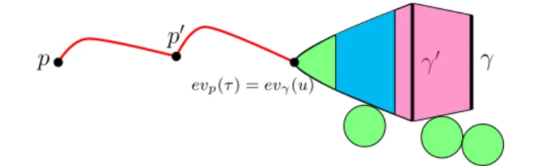
See Figure 1.1 for a diagram of an element of M(p, γ, A).

If all choices can be made so that M(p, γ, A) is smooth (and of the expected dimension), then the coefficient ofP SS(p) on the generator (γ, A) is defined to be the count #M(p, γ, A) if the expected dimension is 0, and the coefficient is 0 otherwise. Now, for general Y, the

(18)

SPACES 10

p p

0

γ0 γ

evp(τ) =evγ(u)

Figure 1.1: An element (τ, u) in the moduli space M(p, γ, A). The red lines represent an element τ ∈ M(p, Y) consisting of a Morse trajectory from ptop0 and a half-infinite Morse trajectory starting at p0 and evaluating to evp(τ) in the unstable manifold of p0. The green near evγ(u) represents the neighborhood of 0 ∈ _C on which the map _C → Y satisfies the

J-holomorphic curve equation. As the map limits to the Hamiltonian orbit γ0, the J-curve equation interpolates in the blue region to Floer’s equation represented in magenta. A Floer trajectory fromγ0 toγhas broken off. The green circles represent bubbled offJ-holomorphic spheres. The evaluations evp(τ) = evγ(u) agree since M(p, γ, A) is a fiber product.

compact moduli space M(γ, A) will not be cut out transversely for anyJ, and hence has no reason to be smooth. Moreover, even if M(γ, A) is cut out transversely, there is no reason to expect that the fiber product with M(p, Y) is transverse.

In [16], these transversality issues are overcome using the results in this paper as follows. The Symplectic Field Theory polyfolds in [18] include polyfold bundles E(γ, A)→X(γ, A) and sc-Fredholm sections

σ(γ, A) :X(γ, A)→E(γ, A) with solution set the SFT moduli space

σ(γ, A)−1(0) =M(γ, A).

HereX(γ, A) is the polyfold of broken and nodal maps of the same form as those inM(γ, A) but not necessarily satisfying any equation, and the sectionσ(γ, A) is the equation that maps inM(γ, A) are required to satisfy. Moreover there is a sc-smooth evaluation map

evγ :X(γ, A)→Y

which evaluates at 0 ∈ _C. This evaluation map is a submersion on the ambient space

X(γ, A), and it restricts to the evaluation map on the moduli spaceevγ :M(γ, A)→Y. Applying the fiber product result Corollary 1.7.3 to the zero section of the rank-0 bundle over the Morse moduli space M(p, Y) and the sc-Fredholm section σ(γ, A), we obtain an open neighborhood X(p, γ, A) of the zero set of the fiber product section

M(p, Y)_ev_p×_ev_γ X(γ, A)→E(γ, A) (τ, u)7→σ(γ, A)(u)

(19)

SPACES 11 such that the restricted section

σ(p, γ, A) :X(p, γ, A)→E(p, γ, A) :=E(γ, A)|X(p,γ,A)

is sc-Fredholm with indexind(σ(p, γ, A)) = dimM(p, Y) +ind(σ(γ, A))−2n. Its zero set is compact and equal to the PSS moduli space

σ(p, γ, A)−1(0) =M(p, γ, A).

The perturbation theory in [34] then provides a sc+-multisection Λ of the polyfold bundle

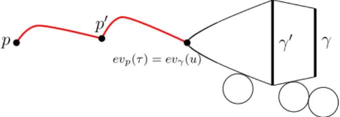
E(p, γ, A) → X(p, γ, A) so that the perturbed solution space S(σ(p, γ, A), Λ) is a smooth compact weighted branched orbifold; see Figure 1.2 for an element of S(σ(p, γ, A), Λ). The weighted count of points in this perturbed moduli space provides the definition of the PSS map. That is, the coefficient of P SS(p) on (γ, A) is given by hP SS(p),(γ, A)i := #S(σ(p, γ, A), Λ).

p p

0

γ0 γ

evp(τ) =evγ(u)

Figure 1.2: An element (τ, u) in the perturbed moduli space S(σ(p, γ, A), Λ) ⊂ M(p, Y)_ev_p×_ev_γ X(γ, A). The red lines represent the broken Morse trajectory τ ∈ M(p, Y) with finite end evaluating to evp(τ). The region from evγ(u) to γ0 is a map C→Y limiting to the Hamiltonian orbit γ0 at ∞. The region in between γ0 and γ represents a cylinder limiting to these orbits on its two ends, and the circles represent attached sphere bubbles. Together the white regions represent the element u ∈ X(γ, A). They are colored white, in contrast to Figure 1.1, to indicate that they do not necessarily satisfy any equation due to the perturbation Λ. The evaluations evp(τ) = evγ(u) still agree since S(σ(p, γ, A), Λ) is contained in the fiber product.

1.1.2.3 Avoiding sphere bubbles in expected dimension 0 and 1

A common mantra in symplectic topology is that “sphere bubbling is a codimension-2 phe-nomenon” and hence sphere bubbles do not appear in regularized moduli spaces of dimension 0 and 1. The notions of a sliced sc-retract (Definition 1.3.2) and a sliced sc-Fredholm germ (Definition 1.3.8) introduced in this paper provide a method for making this precise in the context of polyfold theory.

For simplicity, we consider the case of a curve with 1 interior node, for example a curve with a single sphere bubble. This curve naturally sits inside a _R2-sliced sc-retract (O,_R2×

C,_R2_×

E) which locally models a neighborhood of the curve in an ambient polyfold. TheR2

(20)

SPACES 12 [34, Def. 2.18] obtained from pregluing at the node. In particular, O is homeomorphic to the image of the pregluing map, so conceptually we identify them. Since pregluing with gluing parameter 0∈_R2 _{preserves the node, the induced tame sc-retract ˜}_O₌_{O ∩}₍_{₀_{} ×}_C₎

(Lemma 1.3.3) consists of the curves in O that have 1 interior node. This formalizes the notion that a curve with 1 interior node sits inside a codimension-2 stratum consisting of nearby nodal curves.

Moreover, the Cauchy-Riemann section∂J :O →K of the local bundle modelK → O is a_R2_{-sliced sc-Fredholm germ, and hence by Lemma 1.3.10 its restriction to ˜}_O_{is sc-Fredholm}

with index satisfying ind(∂J|O˜) = ind(∂J)−2. If the original section satisfies ind(∂J) ≤1, i.e. the expected dimension of the moduli space is≤1, then its restriction to the nodal curves in ˜O satisfiesind(∂J|_O˜)<0. So, after perturbing the restricted section, the transversely cut

out zero set must be empty as a smooth object with negative dimension. Extending this perturbation over all of O, the perturbed zero set will not intersect ˜O, meaning that the perturbed zero set will not contain any nodal curves.

This perturbation extension result will be part of a future work, which to be applied must include an inductive procedure that perturbs and extends starting with the highest codimension strata corresponding to solutions with the most nodes. Indeed, a curve with

k ≥1 nodes sits inside the intersection of k distinct codimension-2 strata, and this intersec-tion is a codimension-2k stratum. One must perform the local perturbations and extensions coherently with respect to the intersections of these nodal strata.

Acknowledgments: I am deeply grateful to my PhD advisor, Katrin Wehrheim, for warmly inviting me into this area of research, leading me to fruitful areas to explore, keeping my vision clear as I navigate, and teaching me how to write. Katrin’s support throughout my graduate studies was fundamental to my completion of this research. Additionally, I’d like to thank Helmut Hofer, Wolfgang Schmaltz, and Zhengyi Zhou for useful comments, conversations, and feedback that resulted in improvements to this paper.

1.2

Sc-calculus: the normal form of a local sc-smooth

submersion to

R

n

The purpose of this section is to establish the normal form (Lemma 1.2.3) of a sc-smooth local submersionf : [0,∞)s×_E→_Rn_{, where}

Eis a sc-Banach space. This is a sc-calculus analog of

the classical local submersion normal form (Lemma 1.2.1) in the case where_Eis an ordinary Banach space E. In the Banach case, the normal form follows from the inverse function theorem for C1 maps between open subsets of quadrants [0,∞)s×E. The inverse function theorem does not hold in sc-calculus [17], however, using relationships between classical differentiability and sc-differentiability, we leverage the classical normal form to prove the normal form in sc-calculus. The key ingredient is that the target of these submersions is finite dimensional _Rn_{, on which all sc-structures are trivial (i.e. all levels are isomorphic to}

(21)

SPACES 13 the infinity level).

For completeness, we now provide a proof of the normal form in the classical Banach case. We view a quadrant [0,∞)s ×E as a Banach space with boundary and corners. It suffices to consider neighborhoods in [0,∞)s ×E of a point x that sits in the maximally degenerate cornerx∈ {0} ×E.

Lemma 1.2.1. (Normal form of a C1 _{local submersion to}

Rn) Consider a Banach

space E, an open subset U ⊂ [0,∞)s _×_E _{for some} _s _≥ ₀_{, and a} _C1 _map _f _: _U _→

Rn.

Suppose that, for some x∈ U ∩({0}s_×_E₎_{, the tangent map} ₍_d

xf)|{0}s_×_E :E → _Rn of the

restriction to the corner f|U∩({0}s_×_E₎ is surjective.

Then, for any complementLofK := ker(dxf)|{0}s_×_E inE, there exist open neighborhoods

x∈Uˆ ⊂U and U0 ⊂_Rn_×_[0_,_∞₎s_×_K _{such that, writing} _v _∈_[0_,_∞₎s _and _e_∈_E_{, the map}

g : ˆU →U0

(v, e)7→(f(v, e), v, pr(e))

is a C1-diffeomorphism, where pr:E =K⊕L→K is the projection along L. Proof. Denote the restriction off to the corner by

f :=f|U∩({0}×E) :U∩({0} ×E)→Rn.

Then dxf : E → Rn is surjective by hypothesis. Let L be any complement of K = kerdxf inE. In particular, note that this means the restriction

dxf|L:L→Rn (1.1)

is an isomorphism. Writing v ∈[0,∞)s and e∈E, define the map

g :U →_Rn_×_[0_,_∞₎s_×_K (v, e)7→(f(v, e), v, pr(e)),

where pr :E =K ⊕L→K is the projection along L. Note that g is C1 _since _f _is _C1 _and

pr is C∞.

We claim that the tangent map

dxg :Rs×E →Rn×Rs×K (v, e)7→(dxf(v, e), v, pr(e))

is an isomorphism. To verify injectivity, suppose (0,0,0) = (dxf(v, e), v, pr(e)). Then e ∈ ker(pr) = L, and moreover 0 = dxf(0, e) = dxf(e) means e∈K, hence e = 0. To verify surjectivity, let (p, v, k)∈_Rn_×

Rs×K. Since the map (1.1) is an isomorphism, there exists l ∈Lsuch thatdxf(l) = p−dxf(v, k). It follows that dxf(v, k+l) =dxf(v, k) +dxf(l) =p

(22)

SPACES 14 and hence dxg(v, k+l) = (dxf(v, k+l), v, pr(k+l)) = (p, v, k). So dxg is an isomorphism, as claimed.

Since g is aC1 map whose tangent map dxg atxis an isomorphism, the inverse function theorem1 for C1 maps between quadrants of Banach spaces applies: There exists an open neighborhood ˆU ⊂U of x and an open set U0 ⊂_Rn_×_[0_,_∞₎s_×_K _{such that the restriction}

g|_Uˆ : ˆU →U0 is a C1-diffeomorphism, as claimed.

We briefly review basics about sc-calculus on sc-Banach spaces from [34, Sec. 1.1] to prepare for Lemma 1.2.3. A sc-Banach space [34, Def. 1.1] is a sequence of Banach spaces and continuous linear injections

E:= E0 ←- E1 ←-· · ·

such that the map Em+1 ,→Em is a compact operator for everym≥0 and the intersection

E∞:=∩m≥0Em

is dense in every Em. We call E∞ the smooth points of E. By a subset S of a sc-Banach

space _E we mean a subset S0 of E0, which then induces subsets

Sm :=S∩Em ⊂Em for all m ≥0,

S∞:=S∩E∞ ⊂E∞.

In particular, if U is open in E0 then Um ⊂ Em is open for all m ≥ 0, so we say that U is open in the sc-Banach space _E.

A sc-subspace _F ⊂ _E [34, Def. 1.4] is a closed subspace F ⊂ E0 such that the induced

subsets Fm :=F ∩Em define a sc-Banach space F= (F0 ←- F1 ←-· · ·). Given sc-subspaces

F,F0 ⊂ E such that, for every m ≥ 0, the Banach space Em splits as a direct sum Em =

Fm ⊕Fm0 , we say that there is a sc-splitting E= F⊕F

0 _{and that}

F,F0 are sc-complements

in _E. Given a sc-subspace _F⊂ _E, the quotient space _E/_F has the structure of a sc-Banach space withm-level Em/Fm; see [34, Prop. 1.2]. The following fact is established in the proof of [34, Prop. 1.4]. We reproduce the proof here for completeness.

Lemma 1.2.2. Consider a sc-Banach space _E and a sc-subspace _F ⊂ _E such that the quotient _E/_F is finite dimensional. Then, there exists a sc-complement _F ⊕L = _E and moreover L⊂E∞.

Proof. Consider the sc-continuous quotient map p : _E → _E/_F. Since E∞ ⊂ E0 is a dense

linear subspace and p : E0 → E0/F0 is surjective, it follows that p(E∞) is a dense linear

subspace of the finite dimensional space E0/F0, and so we have p(E∞) = E0/F0. Hence,

choosing any basis of E0/F0, there are preimages of the basis elements in E∞, and these

preimages span a subspace L ⊂ E∞. We claim that L is sc-complementary to F in E.

Indeed, for every m ≥ 0 the subspace Em ⊂ E0 is dense and so pm : Em → E0/F0 is

surjective. Moreover, we have Fm = ker(pm) and the restriction pm : L → E0/F0 is an

isomorphism, so Fm⊕L=Em holds. 1_{See, for example, [39, Thm. 2.2.4].}

(23)

SPACES 15 For every l ≥0 there is al-shifted sc-Banach space defined by

El:= (El←- El+1 ←-· · ·),

that is,

(_El)m =Em+l for all m ≥0.

Conceptually, we are forgetting about finitely many levels. Note that l-shifting does not change the∞-level. Analogously, for any subsetS ⊂_E, we defineSl _⊂

El by (Sl)m :=Sm+l. In particular, if U ⊂_Eis open, then Ul ⊂_El _{is open for all} _l_≥_0.

A Cartesian product _E×_F of sc-Banach spaces has a natural sc-structure with m-level given by (_E×_F)m := Em×Fm equipped with any standard Banach norm on a Cartesian product. In this paper, we use the convention that all norms on Cartesian products are the sum norm ||(·,·)||Em×Fm =|| · ||Em +|| · ||Fm, which is equivalent to all standard choices.

The finite dimensional space _E = _Rn _{has a canonical sc-structure given by} _E

m = Rn equipped with the standard Euclidean norm for every m ≥ 0, and where every inclusion

Em+1 →Em is the identity map.

The tangent space [34, Def. 1.8] of a sc-Banach space_E is the sc-Banach space

T_E:=_E1×_E,

with sc-structure given by (T_E)m = Em+1 ×Em for m ≥ 0. Given an open subset U ⊂ [0,∞)s_×

E for somes ≥0, its tangent space is

T U :=U1×(_Rs×_E).

Consider sc-Banach spaces _E,_F, and open subsetsU ⊂[0,∞)s_×

Eand V ⊂[0,∞)s 0

×_F. Then a map

f :U →V

is called sc0 _or _{sc-continuous} _{[34, Def. 1.7] if, for all} _m _≥ _{0, we have} _f₍_U

m) ⊂ Vm and the map f : Um →Vm is continuous. Asc0 map f :U → V is called sc1 with tangent map [34, Def. 1.9]

T f :T U →T V (1.2)

defined by

T f :U1×(_Rs×_E)→V1 ×(_Rs0 ×_F) (x, ξ)7→(f(x), Dxf(ξ)) if, for every x∈U1_{, there exists a bounded linear operator}

Dxf :Rs×E0 →Rs 0

×F0

such that, for ξ ∈E1 satisfying x+ξ∈U1,

lim

|ξ|1→0

|f(x+ξ)−f(x)−Dxf(ξ)|0

|ξ|1

(24)

SPACES 16 holds, and moreover such thatT f is sc0. Iterating the definition of sc1 yields the notions of sck _for _k _≥_{0 and sc-smooth (denoted sc}∞_{); see the discussion after [34, Def. 1.9].}

An important note is that, for a sc1 map f : U → V and x ∈ U1, the bounded linear operator Dxf : Rs×E0 → Rs

0

×F0 is not necessarily sc-continuous when considered as a

map between sc-Banach spaces Dxf :Rs×E→Rs

0

×_F; that is, continuity on levels higher than 0 can fail. However, if x ∈ U∞ is a smooth point, then by [34, Prop. 1.5] the map

Dxf is indeed a sc-operator [34, Def. 1.2], i.e. a sc-continuous linear map. For this reason, we consider only smooth points x in the following lemma so that the kernel of Dxf is a sc-Banach space as the kernel of a sc-operator.

Lemma 1.2.3. (Normal form of a sc-smooth local submersion to _Rn₎ _{Consider a}

sc-Banach space _E, an open subset U ⊂ [0,∞)s×_E for some s ≥ 0, and a sc-smooth map

f : U → _Rn_{. Suppose that, for some smooth point} _x _∈ _U

∞∩({0} ×E), the tangent map

(Dxf)|{0}×_E:E→Rn of the restriction to the corner f|U∩({0}×_E) is surjective.

Then, for any sc-complement2 L of _K:= ker(Dxf)|{0}×_E in E, there exist open

neighbor-hoods x ∈ Uˆ ⊂ U1 _and _U0 _⊂

Rn×[0,∞)s×K1 such that, writing v ∈ [0,∞)s and e ∈ E1,

the map

g : ˆU →U0

(v, e)7→(f(v, e), v, pr(e))

is a sc-diffeomorphism, where pr :_E=_K⊕L→_K is the projection alongL. Moreover, for all m≥0, the map g|_Uˆ_m : ˆUm →Um0 is a Cm+1-diffeomorphism.

In particular, the following statements hold:

• The composition f◦g−1 _:_U0 _→

Rn is projection onto the Rn-coordinate.

• g preserves the [0,∞)s_-coordinate.

Proof. We claim that the Banach space E1 (the 1-level of the sc-Banach space E), the open

subset U1 ⊂[0,∞)s×E1, and the C1-map

f1 :=f|U1 :U1 →R

n

satisfy the hypotheses of Lemma 1.2.1 (the local submersion normal form in the classical Banach case) at the given point x. First of all, the map f1 is indeed C1 by [34, Prop. 1.7].

By [34, Prop. 1.5], we have dxf1 = (Dxf)|Rs×E1.

We now deduce the surjectivity of the tangent map

(dxf1)|{0}×E1 = (Dxf)|{0}×E1 :E1 →R

n

. (1.3)

By hypothesis, the map (Dxf)|{0}×E0 is surjective. Then sinceE1 ⊂ E0 is dense, it follows

that (Dxf)|{0}×E0(E1) is a dense linear subspace of R

n_{and hence is equal to}

Rn, proving the

claimed surjectivity of the map (1.3). 2_{A sc-complement}_L_of

Kexists by Lemma 1.2.2, since the surjection (Dxf)|{0}×E:E→R

n _{induces an}

(25)

SPACES 17 Let L ⊂ E∞ be any sc-complement of K = ker(Dxf)|{0}×E in E, which exists by

Lemma 1.2.2 since the surjection (Dxf)|{0}×_E :E→Rn induces an isomorphism E/K∼=Rn.

In particular, on the 1-level, we haveK1⊕L=E1. Notice that K1 is the kernel of the map

(1.3).

We have shown that the map f1 satisfies the hypotheses of the classical local submersion

normal form (Lemma 1.2.1), yielding an open neighbhorhood ˆU ⊂ U1 of x and an open

subset U0 ⊂_Rn_×_[0_,_∞₎s_×_K

1 such that, writing v ∈[0,∞)s and e∈E1, the map

g : ˆU →U0

(v, e)7→(f1(v, e), v, pr(e))

is a C1-diffeomorphism, where pr:E1 =K1⊕L→K1 is the projection along L.

We may view ˆU and U0 as open neighborhoods in the sc-calculus sense, i.e. ˆ

U ⊂[0,∞)s×_E1 _and _U0 _⊂

Rn×[0,∞)s×K1.

We claim thatg is a sc-diffeomorphism. First of all, it is sc-smooth sincef1 is sc-smooth by

hypothesis and since the projection pr :_E1 ₌

K1⊕L→K1 is sc-smooth.

To show that g−1 is sc-smooth, we show that it satisfies the conditions of [34, Prop. 1.8]. Letm, l ≥0. We must show that g−1 _{induces a map} _g−1_|

U0

m+l :U

0

m+l→Uˆm that is Cl+1. It suffices to show that, for all m ≥ 0, g−1 _{restricts to a} _Cm+1_-map _g−1_|

U0

m : U

0

m →Uˆm, because then given m, l ≥ 0 the composition U_m0 ₊_l g

−1

−−→ Uˆm+l ,→ Uˆm is Cm+l+1 since the inclusion ˆUm+l ,→ Uˆm is continuous and linear hence C∞. So, to complete the proof of the lemma, it suffices to show that

g : ˆUm →Um0 is a Cm+1_{-diffeomorphism for all} _m_≥_0.

By [34, Prop. 1.7], the restriction

f|_Uˆ_m : ˆUm = ˆU ∩(Rs×Em+1)→Rn

is Cm+1. It follows that the restriction

g|_Uˆ_m : ˆUm →Um0 is Cm+1.

To see that g|_Uˆ_m : ˆUm → Um0 is a bijection, note first that injectivity holds since it is a restriction of the bijectiong. To see surjectivity, note first that, sinceg is surjective onto all of U0, it suffices to show thatg(v, e)∈U_m0 =⇒ (v, e)∈Uˆm.Note that Um0 ⊂Rn×[0,∞)s×

Km+1. So, from the definition of g, we haveg(v, e)∈Um0 =⇒ pr(e)∈Km+1 ⊂Em+1. Since

e−pr(e)∈L⊂E∞,we conclude thate∈Em+1.Hence indeed (v, e)∈Uˆm = ˆU∩(Rs×Em+1)

holds, proving surjectivity of g|_Uˆ_m onto Um0 . The same reasoning shows that the classical tangent map

d(g|_Uˆ_m) : ˆUm×(Rs×Em+1)→Um0 ×(R n_×

(26)

SPACES 18 is bijective. The inverse (g−1)|U0 m = (g|Uˆm) −1 _:_U0 m →Uˆm

is Cm+1 because it is the inverse of a Cm+1 map with invertible derivative. We have shown that g|_Uˆ_m : ˆUm →Um0 is a Cm+1-diffeomorphism, completing the proof of the lemma.

We briefly review general partial quadrants, which up to a linear change of coordinates are the same as the standard quadrants (1.5), i.e. of the form [0,∞)s×_Efor some sc-Banach space _E. This level of generality makes constructions more convenient and is equivalent to working with standard partial quadrants only.

A partial quadrant [34, Def. 1.6] in a sc-Banach space _Eis a closed convex subset C ⊂_E

such that there exists another sc-Banach space _E0 and a linear sc-isomorphism

Ψ :_E→_Rs_×

E0 satisfying Ψ(C) = [0,∞)s×E0 for somes ≥0. (1.4)

That is, all partial quadrants come from applying a linear change of coordinates to a partial quadrant in the standard form:

C = [0,∞)s×_E0 ⊂_Rs×_E0 =_E. (1.5)

The degeneracy index [34, Def. 1.10]dC :C →N0 is defined for x∈C by

dC(x) := #{i∈ {1, . . . , s} |the i-th coordinate of Ψ(x) is 0},

which is independent of the choice of Ψ by [34, Lem. 1.1]. Conceptually, the degeneracy index of a point in a partial quadrant is the local notion of boundary and corner index in a

M-polyfold.

Later, we need the following properties of the degeneracy index. Let C be a partial quadrant of a sc-Banach space _E and n ≥0. Then _Rn×C is a partial quadrant of _Rn×_E

and

d_Rn_×_C(p, x) =d_C(x) for all (p, x)∈_Rn×C. (1.6) LetCi be a partial quadrant ofEi fori= 1,2.Then C1×C2 is a partial quadrant ofE1×E2

and

dC1×C2(x1, x2) = dC1(x1) +dC2(x2) for all (x1, x2)∈C1×C2. (1.7)

We recall from [34, Def. 2.16] the following linear sc-subspace _Ex ⊂ E associated to a point xin a partial quadrant C ⊂_E. First assume thatC is in the standard form (1.5) and write x= (x1, . . . , xs, ex)∈C. Then, the sc-subspace

Ex :={(v1, . . . , vs, e)∈Rs×E0 | vi = 0 if xi = 0} ⊂E (1.8) conceptually is the tangent space of the intersection of all of the faces of C that contain x. For a general partial quadrant C ⊂_E and x∈C, the subspace _Ex ⊂E is given by

Ex:=Ψ−1((Rs×E0)Ψ(x)), (1.9)

(27)

SPACES 19

1.3

Slices: the local picture

1.3.1

Sliced sc-retracts

In this section, we introduce the new notion of_Rn_{-sliced sc-retracts (Definition 1.3.2), which} we use later as the local models in our definition of a slice ˜B ⊂ B (Definition 1.5.7) of a tame M-polyfoldB (Definition 1.5.1). We prove in Lemma 1.3.3 that a _Rn-sliced sc-retract

O induces a tame sc-retract ˜O ⊂ O which has codimension-n tangent spacesTxO ⊂˜ TxO at every x ∈ O˜1. The global definition of a slice ˜B ⊂ B is then a subspace such that around

every point x ∈ B˜ there is a M-polyfold chart to a _Rnx_{-sliced sc-retract} _O _{that locally} identifies ˜B with the induced tame sc-retract ˜O.

We first recall the local structure of tameM-polyfolds: tame sc-retracts (Definition 1.3.1). Consider a relatively open subset U of a partial quadrant C in a sc-Banach space _E. A sc-smooth mapr:U →U satisfyingr◦r=r is called asc-smooth retraction (or sc-retraction)

[34, Def. 2.1] on U, and the image O :=r(U) of such a map is called a sc-smooth retract (or sc-retract). The triple (O, C,_E) is also called a sc-retract [34, Def. 2.2].

We note that the notion of a smooth retract makes sense in the classical Banach space setting, i.e. given an ordinary Banach space E, we can define a smooth retract O to be any image O = r(U) of a smooth map r : U → U that satisfies r ◦r = r, where U ⊂

[0,∞)s _×_E _{is open. However, modeling spaces on these smooth retracts reproduces the} definition of a Banach manifold because, by [34, Prop. 2.1], a smooth retractOis aC∞ -sub-Banach manifold ofE. The sc-retracts can have much more complicated structure, including locally varying dimension. This is a key difference between classical differentiability and sc-differentiability which allows M-polyfolds to have local dimension jumps and other non-manifold-like structure. Polyfolds arising in applications have these local dimension jumps near broken and nodal curves.

A map ϕ:O → O0 _{between sc-retracts (}_O_{, C,}

E) and (O0, C0,E0) is calledsc-smooth [34,

Def. 2.4] if the compositionϕ◦r:U → O0 _⊂

E0 is sc-smooth as a mapU →E0, whereU ⊂C

is open and r :U → U is any sc-retraction onto r(U) =O. This definition is independent of the choice of open set U and sc-retraction r by [34, Prop. 2.3]. The chain rule holds for sc-smooth maps between sc-retracts; see [34, Thm. 2.1].

The tangent space [34, Def. 2.3] of a sc-retract (O, C,_E) is the image

TO:=T r(T U), (1.10)

wherer :U →U is any sc-retraction on some open subset U ⊂C with image r(U) = O and

T r : T U →T U is the tangent map (see (1.2)) of r. The tangent space TO is well-defined, i.e. independent of U and r, by [34, Prop. 2.2]. The tangent space at x∈ O1 is

TxO =Dxr(TxU). (1.11)

For a smooth point x ∈ O∞, the tangent space TxO is a sc-Banach space since Dxr is a sc-operator. The reduced tangent space [34, Def. 2.15] is the subspace of TxO defined by

(28)

SPACES 20 where _Ex ⊂ E is the subspace from (1.9). Conceptually, TxRO consists of those tangent vectors that point in directions that preserve the degeneracy index, i.e. they lie along the intersection of all of the local faces that contain x. Note that in [34, Def. 2.15] the reduced tangent space is only defined at smooth pointsx∈ O∞. This is because T_xRO can be proven to be invariant under sc-diffeomorphisms ϕ:O → O0_{, i.e.} _D

xϕ(TxRO) =TϕR(x)O

0 _{holds, only}

for smooth points x; see [34, Prop. 2.8]. This invariance proves that the reduced tangent space at a smooth point in a M-polyfold is well-defined, i.e. independent of the chart. The invariance is proven using the characterization [34, Lem. 2.4] of the reduced tangent space

TR

x O at smooth pointsx∈ O∞ as the closure of the space of derivatives of sc-smooth paths

γ : (−, ) → O satisfying γ(0) = x. This only works for smooth points x ∈ O∞ since the image of any sc-continuous map (−, ) → O is contained in O∞ because (−, ) ⊂ _R has the trivial sc-structure where all levels are equal.

As discussed in [34], we must require sc-retractions to be well-behaved with respect to the boundary faces of the partial quadrant C in the following way in order for the full polyfold machinery to work as required in applications.

Definition 1.3.1. [34, Def. 2.17] Consider an open subset U of a partial quadrant C of a sc-Banach space _E. A sc-retraction r:U →U is called a tame sc-retraction if it satisfies the following conditions:

(1) dC(r(x)) =dC(x) for all x∈U.

(2) At every smooth point x∈ O∞=O ∩E∞, there exists a sc-subspace A⊂E such that E=TxO ⊕A and A⊂Ex (see (1.9) for Ex).

If so, then the sc-retract O = r(U) is called a tame sc-retract (and so is the triple

(O, C,_E)).

We introduce the following new notions of _Rn_{-sliced sc-retractions and}

Rn-sliced

sc-retracts.

Definition 1.3.2. Consider a partial quadrantC of a sc-Banach space _Eand an open subset

U ⊂ _Rn _×_C _{for some} _n _≥ ₀_{. A tame sc-retraction} _r _: _U _→ _U _{is called a}

Rn-sliced

sc-retraction if it satisfies

π_Rn◦r =π

Rn on U, (1.13)

i.e. r preserves the _Rn-coordinate.

If so, then the tame sc-retract O =r(U) (and the triple (O,_Rn_×_C,

Rn×E)) is called a Rn-sliced sc-retract.

In the following lemma, we show that for any _Rn_{-sliced sc-retract} _O _in

Rn×C, the set

˜

O :=O ∩({0} ×C) is a tame sc-retract. Later, we use the inclusion ˜O ⊂ O to define the local models for a slice ˜B ⊂ B (Definition 1.5.7), which is our new notion of aM-polyfold ˜B

embedded with finite codimension in an ambient M-polyfold B.

Lemma 1.3.3. Consider a partial quadrant C of a sc-Banach space _E and a _Rn_-sliced

(29)

SPACES 21

Then, for any open subset U ⊂_Rn_×_C _and

Rn-sliced sc-retraction r :U →U such that r(U) =O, the set U˜ :=U∩({0} ×C) is open in C and the restriction

˜

r :=r|_U˜ : ˜U →U˜

is a tame sc-retraction onto O˜ := ˜r( ˜U). We call r˜the tame sc-retraction induced by r. Moreover,

˜

O =O ∩({0} ×C) (1.14)

holds, so in particular O˜ does not depend on the choices of U and r. We may view O˜

as a subset of C, and we call ( ˜O, C,_E) the tame sc-retract induced by the _Rn-sliced sc-retract (O,_Rn_×_C,

Rn×E).

At everyx∈O˜1, the inclusionO ⊂ O˜ induces an inclusion of tangent spacesTxO ⊂˜ TxO

satisfying

TxO˜ =TxO ∩({0} ×E), (1.15)

T_xRO˜ =T_xRO ∩({0} ×_E), (1.16)

and

TxO/TxO ∼˜ =Rn. (1.17)

We say that O˜ is codimension-n in O.

Ifx∈O∞˜ is a smooth point, then the inclusionTxO˜,→TxO induces a linear isomorphism

TxO˜/TxRO ∼˜ =TxO/TxRO. (1.18)

Proof. The defining property (1.13) of the _Rn-sliced sc-retraction r implies r( ˜U) ⊂ U˜, so indeed the map ˜r := r|_U˜ : ˜U → U˜ takes values in ˜U. Moreover, ˜r inherits sc-smoothness

and the retraction property ˜r◦ r˜ = ˜r from the corresponding properties of r. So ˜r is a sc-retraction onto the sc-retract ˜O. We prove the other statements in the lemma before showing that ˜r is tame.

We now verify that (1.14) holds. The forwards inclusion is immediate from the definitions of the sets involved. To prove the reverse inclusion, letx∈ O ∩({0} ×C).Then since O ⊂U

we have x ∈ U˜ and so ˜r(x) ∈ O˜. We claim that x = ˜r(x), proving (1.14). Indeed, since

x∈ O and r is a retraction with image O, it follows that x=r(x) = ˜r(x).

We now verify (1.15) and (1.17). Let x∈O˜1. By definition of tangent space (1.11) of a

sc-retract, we have

TxO =Dxr(Rn×E)⊂Rn×E.

Sincerpreserves the_Rn-coordinate by the sliced retraction property (1.13), the same is true forDxr,from which it follows thatDxr(Rn×E)∩({0} ×E) =Dxr({0} ×E). Hence we have

(30)

SPACES 22 proving (1.15). Moreover, the projection π : TxO → Rn to the first factor of Rn×E is a

surjection. Since ker(π) = TxO ∩({0} ×E), we conclude that π induces an isomorphism

TxO/TxO ∼˜ =Rn, proving (1.17).

To verify (1.16), first note that by (1.8),(1.9), we have

(_Rn×_E)x∩({0} ×E) = ({0} ×E)x, (1.19) and hence we have TR

x O˜ =TxO ∩˜ ({0} ×E)x =TxO ∩˜ (Rn×E)x∩({0} ×E) =TxO ∩(Rn×

E)x∩({0} ×E) =TxRO ∩({0} ×E), as required.

To verify (1.18), it suffices to consider the casex= 0 andC = [0,∞)s×_E0 _⊂

Rs×E0 =E

is in standard form (1.5). By (1.8), we have (_Rn_×

Rs ×E0)x = Rn × {0}s ×E0. Since r preserves the degeneracy index by Definition 1.3.1, we claim it follows that

Dxr(Rn× {0}s×E0)⊂Rn× {0}s×E0. Indeed, given a smooth pointξ∈_Rn_×{₀_}s_×_E0

∞, there exists a sc-smooth pathα : (−, )→

U ∩(_Rn_{× {}₀_}s_×

E0) satisfying α(0) =xand α0(0) =ξ. Sincer preserves degeneracy index

we have r◦α((−, ))⊂ _Rn_{× {}₀_}s_×

E0, and hence we have Dxr(ξ)∈ Rn× {0}s×E0. For an arbitrary pointξ ∈_Rn_{× {}₀_}s_×

E0 the result follows by considering a sequence{ξk}k≥0 of

smooth points that converges to ξ, which exists by density of the inclusion E_∞0 ⊂E₀0. Note that this essentially uses the fact that xis a smooth point.

Since by definition (1.12) we have T_xRO = Dxr(Rn ×Rs ×E0)∩(Rn× {0}s ×E0) and

moreover the retraction property Dxr◦Dxr=Dxr holds, it follows that

T_xRO =Dxr(Rn× {0}s×E0).

Hence, since Dxr preserves the Rn-coordinate, the projection π : TxO → Rn restricts to a surjection π : T_xRO → _Rn_{. The kernel of this surjection is} _TR

x O˜ by (1.16). So we have a short exact sequence of sc-Banach spaces 0 →TR

x O →˜ TxRO π

−

→ _Rn _→ _{0 that includes into} the short exact sequence 0→TxO →˜ TxO

π

−

→_Rn_. _{This implies (1.18).}

To prove the lemma, it remains to show that ˜r is tame. The _Rn-sliced sc-retraction r

is tame by definition. Hence, for all x ∈ U˜, we compute, using (1.6) and property Defini-tion 1.3.1(1) ofr,

d{0}×C(˜r(x)) = dRn×C(˜r(x)) =dRn×C(r(x)) =dRn×C(x) =d{0}×C(x), verifying property Definition 1.3.1(1) for ˜r.

To verify that ˜r satisfies property Definition 1.3.1(2), let x∈O∞˜ . Then x∈ O∞, and so by the corresponding property of r and by [34, Prop. 2.9], the sc-subspace A := (id_Rn_×

E−

Dxr)(Rn×E) ofRn×E satisfies

Rn×E=TxO ⊕A (1.20)

and A⊂(_Rn_×

E)x. By the sliced retraction property (1.13) ofr and the definition ofA, we conclude that A ⊂ {0} ×_E holds. Then we have A⊂ (_Rn_×

(31)

SPACES 23 by (1.19). We claim that {0} ×_E = TxO ⊕˜ A holds, completing the proof that ˜r is tame. Indeed, it follows from (1.15), (1.20), and A⊂ {0} ×_Ethat we have

{0} ×_E= (TxO ∩({0} ×E))⊕A=TxO ⊕˜ A.

1.3.2

Sliced bundle retracts

In this section, we introduce the new notion of _Rn-sliced bundle retracts (Definition 1.3.4). We prove in Lemma 1.3.5 that a _Rn_{-sliced bundle retract} _K _{covering a}

Rn-sliced sc-retract

O induces a tame bundle retract ˜K ⊂K covering the induced tame sc-retract ˜O ⊂ O from Lemma 1.3.3. The global definition of a slice ˜B ⊂ B of a bundle ρ:E → B (Definition 1.5.7) is then a subspace such that around every point x ∈ B˜ there is a bundle chart for ρ to a _Rnx_{-sliced bundle retract} _K _{that locally identifies} _ρ−1_{( ˜}_B_{) with the induced tame bundle} retract ˜K.

We first recall the local structure of tame strong bundles: tame bundle retracts. Consider a relatively open subset U of a partial quadrant C of a sc-Banach space _E, and another sc-Banach space _F. Then the trivial bundle

U _F→U (1.21)

has total space U _F=U ×_F as a set, and the map is projection onto U. The triangle signifies the extra structure of a double filtration on the setU×_F. That is, for 0≤k ≤m+1, we have

(U _F)m,k :=Um⊕Fk. Then, for i= 0,1, we define the sc-structure (U _F)[i] by

((U _F)[i])m :=Um⊕Fm+i, m ≥0. (1.22) The purpose of defining these two filtrations is that they correspond to the two notions of smoothness of a section of a bundle that are important for polyfold theory. Precisely, a section s : U → U _F is called sc-smooth if it is sc-smooth as a map to (U _F)[0]. If, moreover, we have s(U)⊂ (U _F)[1] and the map s: U →(U _F)[1] is sc-smooth, then s

is called a sc+_-section_{. See [34, Def. 2.24] for a detailed discussion.}

A strong bundle map Φ: U _F→ U0 _F0 [34, Def. 2.22] is a map which preserves the double filtration and is of the form Φ(x, ξ) = (ϕ(x), Γ(x, ξ)), where the mapΓ :U_F→_F0

is linear in ξ. In addition, for i= 0,1, we require that the maps

Φ: (U _F)[i]→(U0_F0)[i]

are sc-smooth. A strong bundle isomorphism is an invertible strong bundle map whose inverse is also a strong bundle map.

(32)

SPACES 24 To extend (1.21) to a notion of a trivial bundle over a sc-retract, we employ the following notion of a retraction in the fibers. A strong bundle retraction is a strong bundle map

R:U _F→U _Fsatisfying R◦R =R. As a consequence, the mapR has the form

R(x, ξ) = (r(x), Γ(x, ξ)), (1.23) where r : U → U is a sc-smooth retraction and Γ(x,·) : _F → _F is a linear projection for every x ∈ U. If r is tame, then R is called a tame strong bundle retraction. The image K := R(U _F) of R is called a strong bundle retract [34, Def. 2.23], as is the triple (K, C_F,_E_F). We say that K covers the sc-retract O = r(U). If R is tame, then K is called a tame strong bundle retract. The projection U_F→U induces a mappingK → O, which we call a strong local bundle model.

We now introduce the new notion of a _Rn_{-sliced bundle retract.}

Definition 1.3.4. Consider a partial quadrant C of a sc-Banach space _E, an open subset

U ⊂_Rn_×_C _{for some} _n_≥₀_{, and another sc-Banach space}

F.

A tame bundle retraction R :U _F→U _F is called a _Rn-sliced bundle retraction

if the tame sc-retraction r : U → U covered by R (see (1.23)) is a _Rn_{-sliced sc-retraction}

(Definition 1.3.2).

If so, then the tame bundle retractK =R(U_F)(and the triple (K,_Rn×C_F,_Rn×_E

F)) is called aRn-sliced bundle retract and the tame local bundle model K → O :=r(U)

is called a _Rn_{-sliced local bundle model}_.

In the following lemma, we show that for any _Rn_{-sliced bundle retract} _K _in

Rn×CF,

the set ˜K :=K∩({0} ×C_F) is a tame bundle retract. Later, we use the inclusion ˜K ⊂K

to define the local models for the restriction of a bundle to a slice (Definition 1.5.7).

Lemma 1.3.5. Consider a partial quadrant C of a sc-Banach space _E, another sc-Banach space _F, and a _Rn_{-sliced bundle retract} ₍_K,

Rn×C F,Rn×EF) covering a Rn-sliced

sc-retract (O,_Rn ×C,_Rn× _E). Let π : K → O denote the local bundle model given by restriction of the projection along the fiber _Rn_×_C

F→Rn×C.

Then, for any open subset U ⊂_Rn_×_C _and

Rn-sliced bundle retractionR :UF→UF

covering a _Rn-sliced sc-retraction r : U → U such that r(U) = O and R(U _F) = K, the set U˜ :=U∩({0} ×C) is open in C and the restriction

˜

R:=R|_U˜_F : ˜U F→U˜F

is a tame bundle retraction onto K˜ := ˜R( ˜U _F) covering the induced tame sc-retract

Polyfolds and Persistence

UC Berkeley Electronic Theses and Dissertations

Title

Contents

Acknowledgments

Chapter 1

Introduction

SPACES 3

Results

SPACES 5

Applications

SPACES 10

Sc-calculus: the normal form of a local sc-smooth

SPACES 19

Slices: the local picture

SPACES 21

Sliced bundle retracts