Faculty of Business and Law
School of Accounting, Economics and FinanceECONOMICS SERIES
SWP 2011/1
Improving forecasting performance by window
and model averaging
Prasad S Bhattacharya
and Dimitrios D Thomakos
The working papers are a series of manuscripts in their draft form. Please do not quote without obtaining the author’s consent as these works are in their draft form. The views expressed in this paper are those of the author and not necessarily endorsed by the School or IBISWorld Pty Ltd.
1
Improving forecasting performance by window and model averaging
♦Prasad S Bhattacharya• and Dimitrios D Thomakos♣
Abstract
This study presents extensive results on the benefits of rolling window and model averaging. Building on the recent work on rolling window averaging by Pesaran et al (2010, 2009) and on exchange rate forecasting by Molodtsova and Papell (2009), we explore whether rolling window averaging can be considered beneficial on a priori grounds. We investigate whether rolling window averaging can improve the performance of model averaging, especially when ‘simpler’ models are used. The analysis provides strong support for rolling window averaging, outperforming the best window forecasts more than 50% of the time across all rolling windows. Furthermore, rolling window averaging smoothes out the forecast path, improves robustness, and minimizes the pitfalls associated with potential structural breaks.
Keywords: Exchange rate forecasting, inflation forecasting, output growth forecasting, rolling window, model averaging, short horizon, robustness.
JEL codes: C22, C53, F31, F47, E31
♦
We would like to thank Michael Clements, Mark Wohar and John Guerard Jr. for their insightful comments. Please do not quote without permission. All computations performed in R.
• Corresponding author. Senior Lecturer, Economics, School of Accounting, Economics and Finance,
Deakin University, Melbourne Campus, Australia and Research Associate, Centre for Applied
Macroeconomic Analysis, Australian National University, Australia. E-mail
2
1.Introduction
“In addition to misinterpretation of the new out-of-sample tests for nested models, some of the excess optimism in the literature can be attributed to the failure to check for robustness over different forecast windows. Regardless of whether one uses new or old structural models, single equation or panel specifications, one of the main problems related to the forecastibility of the majority of exchange rates remains - lack of robustness over different time periods.” (Rogoff and Stavrakeva, 2008).
In forecasting, averaging is mainly applied for model averaging, i.e. to combining forecasts generated from different models. Timmermann (2006) provides a recent survey on Bayesian model averaging and Clemen (1989) review a number combining applications in economics, finance, psychology, statistics and management science. Much less widespread is the practice of averaging forecasts generated across different segments of historical data, such as combinations of recursive and rolling window forecasts (as in Clark and McCracken, 2009) or averaging forecasts across both models and rolling windows (as in Pesaran, Schuermann and Smith, 2009). The latter papers in particular have placed renewed emphasis on the value of averaging across rolling windows and rightly so: such averaging makes models and forecasts robust to structural breaks and is faster to implement than the procedures proposed in the former papers.
The present study takes the issue of model and rolling window averaging a step further and illustrates how this approach potentially offers significant advantage in the context of both model validation and forecast robustness. First, we explore why rolling window averaging is a more fruitful approach to follow. This hinges on the fact that researchers have no a priori information regarding the optimal window width for generating forecasts and therefore potential pitfalls of data mining could be avoided. In this context, the results are more ‘believable’ as researchers remain agnostic about the segment of data to be used in making inference and taking a decision. Second, we find that such rolling window averaging is generating much better results than the best individual window forecasts 50% or more of the time in short horizons. Therefore, we could think of averaging as not just a more ‘objective’ approach but a potential ex ante winner in forecast-based model evaluations. Third, the rolling window averaging could enhance model averaging as it allows the forecasting ability of simpler, parsimonious models to improve and potentially dominate the forecasting ability of more complicated models. This is practically helpful as researchers would employ univariate models and then average them without the need to look for a (theoretical or otherwise) justification in applying larger multivariate models. In a recent paper, Clark and McCracken (2010) show that in forecasting US output, prices and interest rate from an VAR framework, the best forecasting performance is coming out from a simple average of projections from a univariate model. Fourth, rolling window averaging, by construction, smoothes out the potential adverse effects of structural breaks in the forecast sample and makes inference more robust. The above issues are important in generating optimal forecasts and forecast-based evaluation of models incorporating economic fundamentals.
3
The literature on exchange rate forecasting is a prime area with established mechanics of generating forecasts from different models based on economic theory (see a recent survey by Cheung, Chinn and Pascual, 2005). Exchange rate models with economic fundamentals span Taylor rule models (see, among others, Molodtsova and Papell, 2009), uncovered interest rate parity or interest rate differential model (see, among others, Clark and West, 2006), monetary fundamentals model (see, among others, Sarno and Velante, 2009, Engel, Mark and West, 2007, Groen, 2005, Rapach and Wohar, 2002, Kilian, 1999, Mark, 1995), purchasing power parity model (see, among others, Rogoff and Stavrakeva, 2008, Papell, 2006 and Mark and Sul, 2001), as well as external balance model (see, among others, Gourinchas and Rey, 2007). However, all these models, in general, are set-up against a vicious opponent that is difficult to beat: the random walk benchmark. Starting with the seminal study of Meese and Rogoff (1983), and recent work by Sarno and Valente (2009), there is evidence of mixed success of outperforming forecasts generated from the benchmark with those of the fundamentals in short horizons. Importantly, and as our initial quote makes amply clear, even if at times the forecasts from fundamentals are better than the benchmark, there is lack of robustness across different time periods (see also Engel and West, 2005). Recently, Giacomini and Rossi (2009) put forward a theoretical framework to deal with the issue of robustness over different forecast windows. In particular, they propose a forecast breakdown test and argue that it takes care of potential structural breaks in parameters, addresses potential instability in the distribution of the regressors and would predict future forecast breakdowns. However, if the researcher’s aim is to produce optimal forecasts, then the forecast breakdown test would not be helpful. This happens as it is difficult to know a priori what the performance of models would be when using different time segments, i.e., the data generating process is changing over time. In such a setup, it would be preferable to consider many different time segments and then average them. Note that this averaging across different windows also enhances, not diminishes, the theoretical foundations of economic models since all models are assumed to hold “on average”.
Forecasting US inflation and output growth is another important area where researchers find frequent evidence of structural break or parameter instability and mixed evidence in outperforming the benchmark (see, among others, Stock and Watson, 2010, Stock and Watson, 2004, and Stock and Watson, 1996). Inflation rate and real output growth rate share a number of similarities with exchange rate but they also have key differences. The similarities are structural breaks in both types of variables and the strong theoretical foundations about which right-hand-side variables could be used as predictors. The differences, on the other hand, focus on the absence of a well-defined (and commonly agreed) benchmark model, the rather differential performance of recursive versus rolling window forecasts and the absence of an ‘all inclusive’ theoretical model (like the Taylor rule type model for exchange rates) with clearly defined economic variables. Instead, there are factors that come out of the work of Stock and Watson (1999, 2002a, 2002b, 2004) and the papers of Clark and McCracken (2010) which resort to these factors in a forecasting context.
In this paper, we first motivate the forecasting across windows and models using a simulation approach. A first-order autoregressive model is used with the intuition that
4
any kind of averaging is meant to smooth-out structural changes and improve forecasting performance. The simulation takes a simple approach to time-variation, by considering a time-varying slope parameter in the autoregression. Therefore, the functional form remains the same throughout but with a changing parameter. The model exhibits structural changes in the parameters, a form commonly addressed by tests on structural changes. Even in this straightforward context it is clear that forecasting with a fixed rolling window (or recursive) will not be appropriate. We show that window averaging improves forecasting performance vis-à-vis fixed rolling window forecasts. In addition, model averaging of recursive and average rolling forecasts also improves performance.
Afterwards, we look at the forecasting performance of rolling window and model averaging with real data. This is done in two parts. In the first part, we expand the extensive work of Molodtsova and Papell (2009) to account for both model and rolling window averaging and to work out the robustness problem outlined in Rogoff and Stavrakeva (2008). Our work on exchange rate models differs qualitatively from the Pesaran et al. papers (2009) since our interest lies in the relative validity of the models themselves, not just the superior forecasting performance. There are 12 OECD countries in the dataset. Molodtsova and Papell (2009) use one non-linear model (based on the Taylor rule) and three linear models (based on interest rate differential, monetary fundamentals and purchasing power parity) and report forecast superiority in short horizon with the Taylor rule model. Using our double averaging method, we find the combination of simpler models based on economic fundamentals outperform the random walk benchmark in a majority of countries. This finding is robust across different rolling window scenarios. Our results directly address the non-robustness issue of Rogoff and Stavrakeva (2008), in particular, in terms of the uncertainty that characterizes model performance and forecasting results based on fixed rolling windows. Note that window averaging takes care of the effects of the fixed (“wrong”) window size but the forecasting results are still dependent on the choice of the forecasting origin and horizon, and these evolve so that the variational uncertainty still remains. Therefore, the window averaging should deal adequately with the problems raised in Rogoff and Stavrakeva (2008) but for fixed forecasting origin and horizon, i.e. its good performance is “conditional” on them. However, this does not invalidate the argument for rolling window averaging, it merely makes the rest of the analysis of forecast errors conditional to the moving sequence of forecasting origins and horizons.
In the second part of the paper, we use FRED data and 10 different models to compute one-period ahead forecasts for US inflation and output growth. The models are in line with Stock and Watson (2003, 2004). Here, we have some evidence that rolling window averaging allows simpler models with economic predictors to perform well and to combine their forecasts well. As before, the finding remains robust across different rolling scenarios. The results resonate with recent findings by Pesaran et al (2009).
The rest of the paper is organized as follows. In section 2, we present a short review of the related literature. Section 3 contains discussion about models, methodology and data.
5
Section 4 reports results from an illustrative simulation study. Forecasting results and discussion from exchange rates, inflation and output growth are discussed in Section 5. Section 6 concludes. All tables are provided in Appendix.
2. A brief overview of literature1
Timmermann (2006) and Stock and Watson (2004) provide overviews of the established literature on forecast improvements using model averaging. Aiolfi, Capistran and Timmermann (2010) argue forecast combinations outperform individual forecasts in presence of unstable model parameters. Clements and Hendry (1998, 1999, and 2006) and Pesaran and Timmermann (2005) also find model instability as an important determinant of forecasting performance and propose forecast combinations to improve forecasts in presence of such parameter instability.
In exchange rate forecasting, recently, Rogoff and Stavrakeva (2008) pool forecasts from a purchasing power parity (PPP) model incorporating persistent cross-country shocks and a driftless random walk model. They find forecasts from model averaging are better than the random walk forecasts 70% of the time. They use exogenously assigned fixed weights to perform the averaging and report superior results from simple averaging. Simple averaging tends to outperform forecasts with endogenously assigned weights (see, the classic study by Bates and Granger, 1969, and the recent discussion in Clements and Hendry, 2004).
In line with the above finding, researchers also report superior forecasting ability from combinations of models in inflation rate and output growth. For instance, Stock and Watson (2004) apply model averaging for seven developed countries (Canada, France, Germany, Italy, Japan, UK and USA) output growth forecast and find the mean squared forecasting errors from a majority of combination forecasts to be always lower than forecasts from the benchmark autoregressive model. They also find the average of combination forecasts is the most robust, as it shows stable performance over time and across countries, and, outperforms individual forecasts coming from a panel setup with the seven countries. Using bivariate models of asset prices for the above seven developed countries, Stock and Watson (2003) show combination forecasts of output growth performing better than the AR benchmark. In particular, for US, at the long horizon (eight-quarter ahead), the combination forecasts of output growth based on the inclusion of asset prices provides robust evidence of best performance. Similar findings are also reported for inflation forecasts involving asset prices in a bivariate modeling setup. On the contrary, Ang, Bekaert and Wei (2007) report for US inflation, combination forecasts are not necessarily better than single model forecasts. To be specific, Ang et al. (2007) show linear combinations of forecasts with weights computed based on past performance and prior information outperform forecasts from simple averaging (i.e., using mean or median).
1 There is a well established literature on economic forecasting (see, among others, Elliot and
Timmermann, 2008), inflation forecasting from the US context (see, among others, Stock and Watson, 2010; Stock and Watson, 2008, Cogley, Primiceri and Sargent, 2010, Stock and Watson, 2007, and Stock and Watson, 2003), and US output growth forecasting (see, among others, Stock and Watson, 2003).
6
Pesaran and Pick (2010) show, in general, averaging of forecasts over different rolling windows from the same model leads to lower forecast bias and lower root mean square forecast error. Pesaran and Timmerman (2007) establish that in presence of structural breaks, one could obtain lower mean squared forecast error using rolling window averaging from the same model. One of the reasons behind rolling window averaging is that it would take care of possible model uncertainty issue involving the optimal size of the estimation window. Additionally, this method would address the very important (and empirically challenging) issue of correctly identifying the break points and measuring the size of the breaks in the forecast. Now, with multiple forecast windows, one would expect breakpoints would be embedded with the averaging, and, therefore, no exact identification of breaks would be necessary (see, Pesaran and Pick, 2010). In a recent paper, Clark and McCracken (2009) argue that averaging across rolling and recursive windows would lead to forecast improvement in presence of a structural break but their approach hinges on bias-variance tradeoff, and, therefore, challenging to implement than the proposed simple window averaging. Researchers are interested in forecast improvement in presence of structural break, as past findings (Paye and Timmermann, 2006; Stock and Watson, 1996) show macroeconomic and financial time series are usually plagued by structural change.
Recently, Rogoff and Stavrakeva (2008) highlight the issue of inconsistent results from different models when different segments of the data are applied. Using three models for exchange rate determination (the Taylor rule as in Molodtsova and Papell (2009), the monetary model as in Engel, Mark and West (2007) and the external balance model of Gourinchas and Rey (2007)), they show inconsistencies in forecasting performance as forecasts from these models cannot outperform forecasts from driftless random walk over all different sample periods. Pesaran et al (2009) use averaging across rolling windows and models to address inconsistencies across sample periods and find that the double averaging procedure produces better results in predicting inflation and output growth within a global VAR context.
3. Models, Methodology and Data
We apply double averaging approach to forecast three important economic variables: (i) exchange rate for 12 OECD countries (as in Molodtsova and Papell, 2009) (ii) output growth for US and (iii) inflation rate for US. For exchange rates, in line with Molodtsova and Papell (2009), we use one non-linear model (Taylor rule model) and three linear models (interest rate, monetary model, and PPP). The benchmark model is the random walk. For US inflation and output growth forecasts, the models are similar to Stock and Watson (2003, 2004) and Clark and McCracken (2009, 2010). A rolling autoregressive model with appropriately chosen lags is the benchmark for inflation and output forecasts. Model specifics are presented below.
3.1. Models for exchange rates
The description of the exchange rate models is taken seriatim from Molodtsova and Papell (2009). We start-off with the Taylor-rule model given in the equation below: Δ𝑠𝑠𝑡𝑡+1 = 𝜔𝜔 − 𝜔𝜔𝑢𝑢𝑢𝑢𝑢𝑢𝑡𝑡 + 𝜔𝜔𝑓𝑓𝑢𝑢𝑢𝑢�𝑡𝑡 − 𝜔𝜔𝑢𝑢𝑢𝑢𝑢𝑢𝑡𝑡 + 𝜔𝜔𝑓𝑓𝑢𝑢𝑢𝑢�𝑡𝑡 + 𝜔𝜔𝑞𝑞𝑞𝑞�𝑡𝑡− 𝜔𝜔𝑢𝑢𝑢𝑢𝑢𝑢𝑡𝑡−1 + 𝜔𝜔𝑓𝑓𝑢𝑢𝑢𝑢̃𝑡𝑡−1 + 𝜂𝜂𝑡𝑡 (1)
7
The dependant variable is the change in the logarithm of nominal exchange rate, at time t+1. The exchange rate refers to domestic price of foreign currency vis-á-vis the US dollar. The notation ~ indicates foreign country variables and the subscripts u and f refer to coefficients for the US and the foreign country respectively. The right-hand-side variables at time t are: 𝑢𝑢𝑡𝑡 the inflation rate, 𝑢𝑢𝑡𝑡 the output gap, 𝑞𝑞𝑡𝑡 the real exchange rate and 𝑢𝑢𝑡𝑡 is the actual, observable interest rate. The output gap is calculated under three alternative scenarios: (a) using deviations from a linear trend, (b) using deviations from a quadratic trend and (c) using deviations from the Hodrick-Prescott filter.2 Taylor rule model is denoted by M1 in the corresponding tables.
The next model is the simple interest rate differential model. This is an important model as it is univariate, represents deviations from parity, and frequently used in assessing the levels of exchange rates. The forecasting equation is obtained by imposing restrictions on the Taylor-rule model above: take 𝜔𝜔𝑢𝑢𝑢𝑢 = 𝜔𝜔𝑓𝑓𝑢𝑢 = 𝜔𝜔𝑢𝑢𝑢𝑢 = 𝜔𝜔𝑓𝑓𝑢𝑢 = 𝜔𝜔𝑞𝑞 = 0 and assume 𝜔𝜔𝑢𝑢𝑢𝑢 + 𝜔𝜔𝑓𝑓𝑢𝑢 = 0 to obtain:
Δ𝑠𝑠𝑡𝑡+1 = 𝜔𝜔 − 𝜔𝜔𝑢𝑢(𝑢𝑢𝑡𝑡 − 𝑢𝑢̃𝑡𝑡) + 𝜂𝜂𝑡𝑡 (2)
where 𝜔𝜔𝑢𝑢 is the common coefficient on the interest rate differential. Note that interest rates do not enter as lagged in the above equation, as is the case with Taylor-rule model. We use M2 to identify this model in the results tables.
Finally there are two additional models, based on monetary fundamentals (depicted as M3 in the discussion tables) and parity fundamentals (denoted by M4 in the results tables), and depend on the deviations of the level of the exchange rate from these fundamentals 𝐹𝐹𝑡𝑡as follows:
Δ𝑠𝑠𝑡𝑡+1 = 𝜔𝜔 − 𝜔𝜔𝐹𝐹(𝐹𝐹𝑡𝑡 − 𝑠𝑠𝑡𝑡) + 𝜂𝜂𝑡𝑡 (3)
where, the fundamentals are determined either by monetary conditions or price deviations as in:
𝐹𝐹𝑡𝑡 = (𝑚𝑚𝑡𝑡− 𝑚𝑚�𝑡𝑡) − 𝑘𝑘(𝑢𝑢𝑡𝑡 − 𝑢𝑢�𝑡𝑡) or 𝐹𝐹𝑡𝑡 = (𝑝𝑝𝑡𝑡 − 𝑝𝑝�𝑡𝑡) (4)
respectively. The above structure assumes purchasing power parity as well as uncovered interest rate parity. All variables are expressed in logarithms. Note that 𝑢𝑢𝑡𝑡 here represents income and not the output gap. Finally, k denotes income elasticity and it takes three fixed values, 0, 1 and 3. In line with Molodtsova and Papell (2009), forecasts are generated under these three income elasticities. Note that when the price deviations are used for the fundamentals we again get a model nested within the Taylor-rule model with the restrictions 𝜔𝜔𝑢𝑢𝑢𝑢 = 𝜔𝜔𝑓𝑓𝑢𝑢 = 𝜔𝜔𝑢𝑢𝑢𝑢 = 𝜔𝜔𝑓𝑓𝑢𝑢 = 𝜔𝜔𝑢𝑢𝑢𝑢 = 𝜔𝜔𝑓𝑓𝑢𝑢=0 and −𝜔𝜔𝐹𝐹 = 𝜔𝜔𝑞𝑞.
In addition to above four individual models, we use the average of all of them and also consider the average of three “simpler” models (except the Taylor rule model) as
8
follows.3 Let the superscripts T, I, M, P denote the four models in the order just presented and let the corresponding forecasts be denoted by 𝑧𝑧̂𝑡𝑡+1|𝑡𝑡𝑚𝑚 = Δ𝑠𝑠�𝑡𝑡+1|𝑡𝑡𝑚𝑚 for m = T, I, M, P. Then, the model averaged forecasts are defined as:
𝑧𝑧̂𝑡𝑡+1|𝑡𝑡𝐴𝐴𝐴𝐴𝐴𝐴 =14�𝑧𝑧̂𝑡𝑡+1|𝑡𝑡𝑇𝑇 + 𝑧𝑧̂𝑡𝑡+1|𝑡𝑡𝐼𝐼 + 𝑧𝑧̂𝑡𝑡+1|𝑡𝑡𝑀𝑀 + 𝑧𝑧̂𝑡𝑡+1|𝑡𝑡𝑃𝑃 � and 𝑧𝑧̂𝑡𝑡+1|𝑡𝑡𝑆𝑆 =13�𝑧𝑧̂𝑡𝑡+1|𝑡𝑡𝐼𝐼 + 𝑧𝑧̂𝑡𝑡+1|𝑡𝑡𝑀𝑀 + 𝑧𝑧̂𝑡𝑡+1|𝑡𝑡𝑃𝑃 � (5)
where the superscript S stands for “simpler”. The average of all models is denoted by M5 and the average of three simpler models is denoted by M6 in the results tables.
3.2. Models for inflation and output growth
We use both monthly and quarterly data for our computations.4 Depending on the data frequency, different measures of inflation rates (monthly, quarterly and annual) and output growth rates (monthly and quarterly) are constructed. Let 𝑃𝑃𝑡𝑡 denote the price variable, 𝑌𝑌𝑡𝑡 denote the output variable, and f denote the frequency of observation. We define 𝑢𝑢𝑡𝑡𝑓𝑓 = Δlog�𝑃𝑃𝑡𝑡/𝑃𝑃𝑡𝑡−𝑗𝑗� and 𝑢𝑢𝑡𝑡𝑓𝑓 = Δlog�𝑌𝑌𝑡𝑡/𝑌𝑌𝑡𝑡−𝑗𝑗� for inflation and output growth, for an appropriate value of j, as:
𝑢𝑢𝑡𝑡𝑀𝑀 = Δlog(𝑃𝑃𝑡𝑡/𝑃𝑃𝑡𝑡−1) – Monthly inflation from monthly data;
𝑢𝑢𝑡𝑡𝑄𝑄 = Δlog(𝑃𝑃𝑡𝑡/𝑃𝑃𝑡𝑡−1) – Quarterly inflation from quarterly data;
𝑢𝑢𝑡𝑡𝐴𝐴 = Δlog(𝑃𝑃𝑡𝑡/𝑃𝑃𝑡𝑡−12) – Annual inflation from monthly data;
𝑢𝑢𝑡𝑡𝑀𝑀 = Δlog(𝑌𝑌𝑡𝑡/𝑌𝑌𝑡𝑡−1) – Monthly growth rates from monthly data;
𝑢𝑢𝑡𝑡𝑄𝑄 = Δlog(𝑌𝑌𝑡𝑡/𝑌𝑌𝑡𝑡−1) – Quarterly growth rates from quarterly data.
All models take the form of an autoregression with a single predetermined variable like the following equation (the m superscript stands for model):
𝑧𝑧𝑡𝑡𝑓𝑓,𝑚𝑚 = 𝛽𝛽0+ 𝛽𝛽1𝑥𝑥𝑡𝑡−1𝑓𝑓,𝑚𝑚 + ∑𝑝𝑝𝑢𝑢=1𝜑𝜑𝑢𝑢𝑧𝑧𝑡𝑡−𝑢𝑢𝑓𝑓 + 𝜂𝜂𝑡𝑡 (6)
where 𝑧𝑧𝑡𝑡𝑓𝑓,𝑚𝑚 is either 𝑢𝑢𝑡𝑡𝑓𝑓 or 𝑢𝑢𝑡𝑡𝑓𝑓 and m denotes the model type, depending on the kind of predetermined variable used. The specifications take the following form:
Inflation
Lags used: p = 1 or 4 for quarterly inflation and p = 1 or 6 or 12 for annual and monthly inflation.
Benchmark: autoregressive model with no predetermined variable (rolling and recursive versions).
Predetermined variables: change in the short-term interest rate, the change in the unemployment rate and the change in output growth (rolling versions only).
3 We use simple averages, as it is a well established result in the literature that combination forecasts with
simple average generally outperforms pooled forecasts with endogenous weights. See the discussion in Rogoff and Stavrakeva (2008, pg. 21) on endogenous versus exogenous weights.
9
Model averages: the pair-wise and total average of the models using each individual predetermined variable; the average of the rolling and recursive version of the benchmark.
Total number of models considered: 10
In the results tables, these models are denoted as M1, M2, M3, M4, M5, M6, M7, M8, M9 and Benchmark. M1 contains autoregressive lags and change in the short-run interest rate. M2 consists of autoregressive lags and change in the unemployment rate. M3 includes autoregressive lags and output growth as regressors. M4 is the average of models M1 and M2, M5 is the average of models M1 and M3, M6 is the average of models M2 and M3, and M7 is the average of models M1, M2 and M3. M8 is a recursive autoregressive model. M9 is the average of rolling and recursive autoregressive lags and Benchmark is a rolling autoregressive model.
Output growth
Lags used: p = 1 or 4 for quarterly growth and p = 1 or 12 for monthly growth.
Benchmark: autoregressive model with no predetermined variable (rolling and recursive versions).
Predetermined variables: change in the short-term interest rate and the change in the unemployment rate (rolling and recursive versions).
Model averages: the average of the rolling and recursive version of the models using each individual predetermined variable; the average of the rolling and recursive versions of both models using the predetermined variables; the average of the rolling and recursive version of the benchmark.
Total number of models considered: 10
In tables, the above models are represented as M1, M2, M3, M4, M5, M6, M7, M8, M9 and Benchmark. M1 contains autoregressive lags of output growth and change in the short-term interest rate. M2 is the recursive version of M1. M3 includes autoregressive lags of output growth and change in the unemployment rate. M4 is the recursive version of M3. M5 is the average of models M1 and M2. M6 is the average of models M3 and M4. M7 is the average of models M1, M2, M3 and M4. M8 is a recursive autoregressive lag model. M9 is the average of rolling and recursive autoregressive lag model and Benchmark is a rolling autoregressive model.
The model averages are defined like the one for exchange rates (see Equation 5). Fixed lag lengths are considered rather than an order selection criterion. This is done to compare the sensitivity of results with respect to different choices of the length of the autoregressive component and to have more output available on the performance of rolling window averaging.5
5
Clark and McCracken (2009) also employ a fixed number of lags in their univariate model specification. Fixed lags are also used in other papers either directly or for comparison with optimized schemes.
A limited analysis (not presented but available on request) with an optimized lag scheme does not alter the qualitative nature of results. Finally, the choice of variables and specifications is partly guided by empirical applications in related literature, as in Stock and Watson (2007, 2008), Athanasopoulos and Vahid (2008), Clark
10
and McCracken (2009, 2010) and others.6 Multivariate models are not considered to maintain comparability with the literature regarding combinations of rolling and recursive forecasts and focuses more on parameter instability7. An immediate extension of current specification would be to use VARs with the same variables as in the individual univariate models.
3.3. Forecasting methodology
Consider M forecasting models and W rolling windows. Each model produces one forecast for each window which is denoted by 𝑧𝑧̂𝑡𝑡+1|𝑡𝑡𝑚𝑚,𝑤𝑤 for m = 1,2,…,M and w = 0,1,2,…,W, where w = 0 denotes the recursive forecast and w = 1,2,… denotes the first, second etc. rolling windows. Details on window magnitude are provided in the discussion of the results. Model averages and rolling window averages are defined in a standard way as illustrated above but for generality we replicate the formulas below. Note that model averaging is always performed first for each rolling window and then the rolling window averaged forecasts are computed.
Forecasts based on model averaging for a given rolling window:
𝑧𝑧̂𝑡𝑡+1|𝑡𝑡𝑀𝑀𝐴𝐴 =𝑀𝑀1 ∑𝑀𝑀𝑚𝑚=1𝑧𝑧̂𝑡𝑡+1|𝑡𝑡𝑚𝑚,𝑤𝑤 (7)
Forecast based on window averaging for a given model (averaging with or without the recursive forecasts depending on the data under analysis; for exchange rates, there are no recursive forecasts):
𝑧𝑧̂𝑡𝑡+1|𝑡𝑡𝑊𝑊𝐴𝐴 =𝑊𝑊1 ∑𝑊𝑊𝑤𝑤=0⋁1𝑧𝑧̂𝑡𝑡+1|𝑡𝑡𝑚𝑚,𝑤𝑤 (8)
Forecast based on model averaging and then on window averaging: 𝑧𝑧̂𝑡𝑡+1|𝑡𝑡𝑀𝑀𝑊𝑊𝐴𝐴 = 1 𝑊𝑊∑𝑊𝑊𝑤𝑤=0⋁1𝑧𝑧̂𝑡𝑡+1|𝑡𝑡𝑀𝑀𝐴𝐴 = 1 𝑀𝑀 1 𝑊𝑊∑𝑀𝑀𝑚𝑚=1∑𝑊𝑊𝑤𝑤=0⋁1𝑧𝑧̂𝑡𝑡+1|𝑡𝑡𝑚𝑚,𝑤𝑤 (9)
M is a variable and it is not fixed throughout our experiments, taking the value of either 2, 3 or 4 depending on the data under analysis. The total number of generated forecasts differs in length according to the window width used. To compute the average forecast the forecasts are trimmed for the same length adjustment (equal to the number of forecasts generated by the largest window width).
The forecasts are always generated one-step ahead but are computed with different, rolling, estimation samples. For example, say we have 300 total observations and we use rolling windows of 100, 120, 130, 150, 170 and 200 observations. We then generate six different one-step ahead forecasts (we align the data correctly, so the first forecast is for period 201 for all estimation windows) and then we average those. The idea here is that
6
See below the discussion on the data section.
11
the forecasts are different since the information sets used to generate them are different, and averaging appears to improve forecasting performance.
The root mean squared error (RMSE) evaluations8 and a variety of appropriate tests are applied to all three types of forecasts. The tests for statistical significance are tailored to the nature of the data. In line with Molodtsova and Papell (2009), we apply the Clark and West (2006) test (denoted by CW) for exchange rates. The asymptotic and bootstrapped versions of the CW test and the Diebold and Mariano (DM) (1995) test are computed for inflation and output growth data. The bootstrapped replications are generated under the benchmark model by the stationary bootstrap of Politis and Romano (1994) where the mean block length is automatically calculated according to Politis and White (2004) and Patton, Politis and White (2009). The simple autoregression (rolling, recursive and average of both) is used as the benchmark model.
3.4. Data
The dataset for exchange rate forecasting is from Molodtsova and Papell (2009)9. The data contain monthly values for money supply, CPI inflation, industrial production, a short-term interest rate and the related exchange rates for 12 OECD countries: Australia, Canada, Denmark, France, Germany, Italy, Japan, Netherlands, Portugal, Sweden, Switzerland and UK. Following Molodtsova and Papell (2009), three measures of output gap are constructed: using linear trend, using quadratic trend and using the Hodrick Prescott filter (HP). Similarly, three different measures of income elasticities (0, 1 and 3) are employed in the monetary fundamentals model.
We use FRED data to forecast US inflation and output growth.10 The change in logarithm of CPI depicts inflation rate.11 Following the literature, the real GDP and industrial production are the measures of output and using these, monthly and quarterly growth rates are calculated. The three-month Treasury bill rate is the short-term interest rate.12 The civilian unemployment rate is the measure for unemployment. For analyzing at the quarterly frequency, we compute quarterly averages of the monthly values for all monthly variables. The total number of initial observations are n = 228 quarters (1953:4 to 2010:1) and n = 472 months (1971:01 to 2010:04).
4. Results from an illustrative simulation
The aim of the simulation is threefold. First, to examine whether rolling window averaging is overall a suitable approach. Secondly, to explore if rolling window averaging is better or not than a recursive scheme. Finally, to see if both model and rolling window averaging outperforms the above two alternatives. For our experiment “model averaging” is based on combining the results from the same model estimated once with a rolling window and then by applying a recursive scheme.
8
See West (2006) for an important update on forecast evaluation.
9 The dataset is downloaded from the web sit
available from Molodtsova and Papell (2009).
10 The web address is:
11
This is described earlier in the methodology section (section 3.2.).
12
We have also experimented with the spread between the 10-year government bond the 3-month Treasury bill rate. The results are available upon request.
12
Since any kind of averaging is meant to smooth-out structural changes and improve forecasting performance, a simple data generating process based on an AR(1) model is considered. This is given by
𝑢𝑢𝑡𝑡 = 𝜑𝜑0+ 𝜑𝜑1𝑡𝑡𝑢𝑢𝑡𝑡−1+ 𝑢𝑢𝑡𝑡 (10)
where the slope parameter 𝜑𝜑1𝑡𝑡 is time-varying by being drawn every 𝑛𝑛𝑡𝑡 observations from the uniform distribution as follows 𝜑𝜑1𝑡𝑡~𝑈𝑈(0.5,1). Therefore, the slope parameter in the model is on average, 𝜑𝜑� = 0.75 with standard deviation 𝑠𝑠𝜑𝜑 = 0.14. We consider three different values for 𝑛𝑛𝑡𝑡 = 20, 40, 60 observations. The intercept parameter is set at 𝜑𝜑0 = 0.5 throughout.
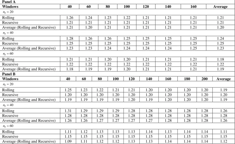
For each of the 500 replications, 240 observations (plus an additional 50 burn-in observations) are simulated from the above model. These are then used to perform a forecasting exercise as follows. First, we define a sequence of rolling windows of sizes {40,60,80,100,120,140,160} and {40,60,80,100,120,140,160,180,200}.13 Thereafter, forecasts are generated based on each individual window, on the average across rolling windows, on the average between each rolling window and the recursive sample and on the average across rolling windows and the recursive sample. 80 forecasts are evaluated for the first rolling window and 40 forecasts are evaluated for the second rolling window. Then mean squared errors (MSE) from all methods are computed and stored at each replication. Finally, the average MSE across all replications are calculated and reported in Panels A and B of Table 1.
Table 1 shows immediate benefit from both rolling window averaging and from model averaging (rolling and recursive scheme combination). It is interesting to note that these results are practically important since the researcher does not know beforehand what the optimal window width is. The rolling window averaging always improves performance compared to the use of any individual window either for the first window or the second window combinations. The double averaging across windows and the recursive scheme has better performance over 67% of the time in comparison to individual windows. In addition, both approaches outperform the recursive estimation scheme and both have about the same performance (out of six cases, in three, the rolling window averaging shows the best overall performance while in the other three cases, the double averaging across windows and models generates the best overall performance).14 These results are robust across rolling windows as well as the choice of 𝑛𝑛𝑡𝑡. Clark and McCraken (2009) show forecasts from combining rolling and recursive windows are better than the forecasts from either a rolling scheme or a recursive scheme with fixed window width. Our results complement the finding from Clark et al (2009).
This experiment is, of course, only indicative of probable improvement with rolling window averaging but it demonstrates such potential exists, especially since it allows one
13 Clark and West (2006) use {60,120,240} observations in their analysis. 14
The performance of the rolling window averaging and the double averaging based on the average MSE is statistically indistinguishable. However, both these approaches provide a statistically significant difference when compared to the recursive scheme.
13
to stay away of the temptation of data mining in order to report the “best performing window”. The question of whether this holds true in a more general setting remains open. We examine this with exchange rate, inflation and output growth data where the data generating processes are unknown and complicated.
5. Results and Discussion
5.1. Results from exchange rate forecasting
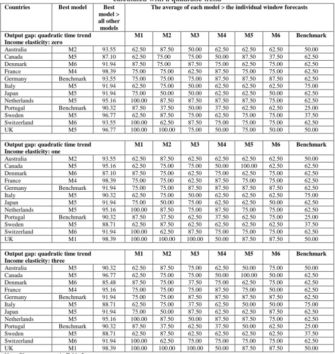
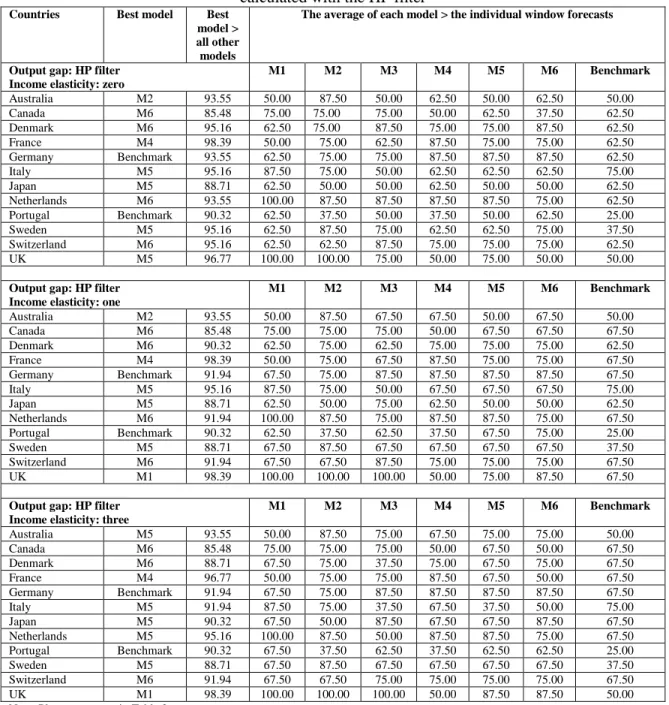
The analysis generated a large volume of results which are available on request but cannot all be discussed here. Therefore, we focus on summaries constructed across different currencies and forecasting models, with the aim of examining whether the rolling window averaging and/or model averaging can outperform the best forecasting model of Molodtsova and Pappell (2009) and the benchmark of the random walk. The summary results appear in Table 2 to Table 7. Table 8 and Table 9 contain results from the application of the Clark and West test for superior forecasting performance.
5.1.1. Results from summary measures for exchange rate forecasting
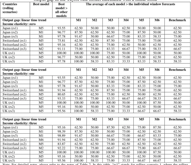
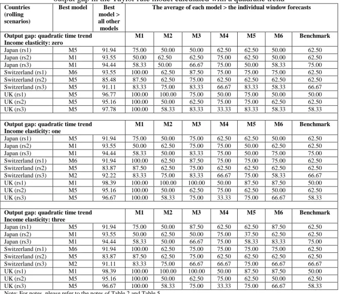
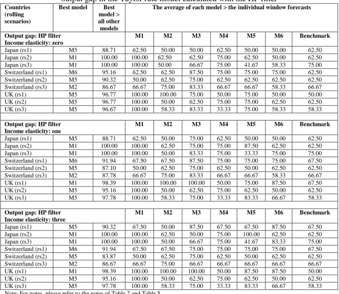
The first overall conclusion by looking at Tables 2 to Table 7 is this: irrespective of which model comes out as the best performing one, the rolling window averaged forecast outperforms the individual window forecasts significantly more than 50% of the time. Specifically, consider all examined individual window forecasts (all models, i.e. all countries and all specifications) and then calculate how many times the rolling window averaged forecast for each model is better than the best individual window forecast. This is a measure of how well the rolling window averaged forecast fared with respect to the individual window forecasts. For each model, we first count whether this measure is greater than 50%.15 Afterwards, the average measure across all models is calculated. We find that in 79% of the examined models, the rolling window averaged forecasts are better than the individual window forecasts by more than 50% of the time (with an average of 74.6% that is significantly different than 50%). This clearly suggests, instead of doing a conditional16 search of the best window length (as in Clark and McCraken, 2009), the researcher can start a forecasting exercise directly by window averaging and be able to outperform significantly more than 50% of the individual windows. Such information allows one to have a priori idea of how to construct appropriate forecasts. This also diminishes the potential pitfalls from ‘window mining’. Furthermore, this result is robust to the number of rolling windows to be averaged and to the length of the smaller window used. We find that in 86% of the examined models, with either a smaller rolling window17 or a larger rolling window18 used instead of the regular rolling window19
15 Cheung, Chinn and Pascual (2005) employ a similar measure in discussing change of directions from
forecasts.
averaged forecasts are better than the corresponding individual window ones (with an
16 The bias-variance tradeoff due to model instability arising out of potential structural break needs to be
taken care of first. See more details in Clark and McCraken (2009).
17 Termed as rolling scenario 2 and denoted by ‘rs2’ in the tables with {120, 132, 144, 156, 168, 180, 192,
204} monthly observations.
18 Termed as rolling scenario 3 and denoted by ‘rs3’ in the tables with {72, 84, 96, 108, 120, 132, 144, 156,
168, 180, 192, 204} monthly observations.
19
Termed as rolling scenario 1 and denoted by ‘rs1’ in the tables with {72, 84, 96, 108, 120, 132, 144, 156} monthly observation.
14
average of 74.4% that is significantly different that 50%). The later finding addresses the key concern in Rogoff and Stavrakeva (2008).
The second overall conclusion is about the ability of rolling window and model averaging to produce competitive or superior results compared to the best model (i.e., the Taylor rule model) of Molodtsova and Pappell (2009). In this context, the forecasting performance of all models using rolling window averaging is considered and the ability of individual model forecasts versus model averaged forecasts is compared. The results are very clear and supportive of both model and window averaging over a single “dominant” model based on a single rolling window. Specifically, and again in context of all examined models, the four individual models (M1, M2, M3 and M4) are ranked as best performers only 18.5% of the time, compared to 16.6% for the benchmark. Furthermore, the monetary model (M3) is never a top performer. The PPP-based model (M4) is ranked as best 8.3% of the time vs. 6.5% of the time for the Taylor rule model (M1) and 3.7% for the interest rate differential model (M2). Clearly, on a single-model comparison, the benchmark model coupled with rolling window averaging is the top performer. This result is important as it shows in presence of rolling window averaging, the dominance of the random walk model comes back! Note that on an ex ante basis it is impossible to identify the appropriate rolling window length to make sure that one of the other models, such as the Taylor rule model, will dominate. A priori, the rolling window averaging seems to be reliable, as it demonstrates the best performance over 50% of the time in comparison to individual rolling windows.
The discussion above also point to one interesting observation regarding models based on fundamentals. The individual models plus the benchmark are ranked the best in only 35.2% of the time. For the rest 64.8% of the cases, the average of all models (denoted by M5) (42.6%) or the average of the three simpler models20 (denoted by M6, 23.2%) are the best models. Therefore, the information contained in economic fundamentals play a vital role in exchange rate forecasting only after model averaging. This finding has a number of important (and practical) implications. First and foremost, it reaffirms the reliance on economic fundamentals in forecasting exchange rate. Sarno and Velante (2009), Engel, Mark and West (2007) and Engel and West (2005) also report reliance on fundamentals in forecasting exchange rates.21
20 These models are: interest rate differential model, monetary fundamentals model and the PPP model,
excluding the Taylor rule model.
Secondly, the ability of simpler, parsimonious models to produce good forecasts when needed is maintained. Thirdly, there is increased robustness in forecasting performance using the double averaging approach. This particular finding resonates with the results from Rogoff and Stavrakeva (2008), especially for Australia and Canada. Rogoff and Stavrakeva (2008) call for a closer look at these two countries when they pooled forecasts from their PPP specification. Our results for Australia and Canada, then, could be seen as a reaffirmation of their concerned cases. Fourth, one does not have to make ex ante search to validate the in-sample performance of various models and window lengths.
21
But note that their modelling setup is very much different than us. See the recent discussion in Sarno and Velante (2009) regarding the support, as well as scepticism, of economic fundamentals in forecasting exchange rates.
15
The combination of the two general results as well as the observation outlined above strongly supports the arguments at the beginning of the paper, namely, the substantial ex ante uncertainty of a suitable forecasting model and of a corresponding window length would be mitigated by a double averaging procedure: rolling window and model averaging. Furthermore, the results support using simpler models along with rolling window averaging, even if the simpler model is the random walk benchmark. That is, rolling window averaging benefits all models, including the benchmark.
5.1.2. Results from Clark and West test for exchange rate forecasting
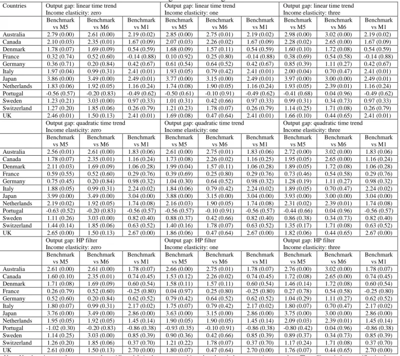
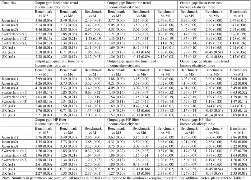
An important issue raised in the existing papers (see, for instance, Molodtsova and Papell, 2009; Rogoff and Stavrakeva, 2008) is that of the relative statistical significance of MSE improvements over the benchmark models. This issue is examined using the CW test statistic for nested models22, since the benchmark is the random walk. We compare the relative statistical significance using results after rolling window averaging is applied to all models and taking the model averaged forecast of all models (M5), the model averaged forecasts of the three simpler models (M6) and the forecast of the Taylor rule model (M1) – all against the benchmark. In all cases and combinations examined23, we consistently find that the model averaged forecast across all models (M5) is outperforming the benchmark a majority of times. The Taylor rule model is not a good performer in comparison to M5. At the 5% (10%) level of significance, the forecasts from M5 are statistically different from the benchmark 30.1% (54.2%) of the time, the forecasts from M6 are statistically different 30.1% (50.1%) of the time and the Taylor rule forecasts are statistically different 28.3% (38.3%) of the time respectively. In addition, the median p-value of the tests is 8.4% for forecasts from M5, 9.2% from the forecasts from M6 and 30.6% from the Taylor rule model forecasts. Note that the calculations refer to forecasts obtained after rolling window averaging where the domination of model averaging over the Taylor rule model is clear from the previous discussion. This implies once rolling window averaging is applied, statistical significance essentially remains only for the model averaged forecasts (M5 or M6) and not for the Taylor rule ones.
5.2.Results from inflation and output growth
A possible constraint on the above results would be that they pertain to specific data and forecasting models. It is, of course, natural to consider other data and models to compare whether the general conclusions remain true in a different context. We thus turn into the discussion of the results on the forecasting performance of models for US inflation and output growth. To preview, the results are also supportive of double averaging but there are differences with respect to their strength. However, note that the breadth of models and data for inflation and output growth forecasts are substantially smaller than the ones involving exchange rates. In this overall discussion results from monthly, quarterly and annual forecasting models are pooled together. Additional comments on their differences are outlined at the end. The results are collected in Table 10 through Table 13. The summary measures and robustness results are presented in Table 10 and Table 11. Table
22
As advised by Clark and West (2006) and subsequently used by, among others, Molodtsova and Papell (2009) and Rogoff and Stavrakeva (2008).
16
12 and Table 13 contain the bootstrapped Clark and West and Diebold and Mariano tests.24
5.2.1. Results from summary measures for inflation and output growth forecasting
As before, we first look at the superior forecasting ability of rolling window averaged forecasts in comparison to individual window forecasts. The results are not as strong as in the exchange rates case. They also differ between forecasts for inflation and output growth.
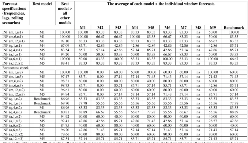
Inflation forecasting results (see Table 10), are, on an average, similar with the results for exchange rates. The top performing model is the one with both rolling window and model average. Pesaran et al (2009) report similar findings regarding inflation from both model and window averaging using a global VAR model. In our analysis, the top performing model after rolling window averaging is (unsurprisingly) the one using the short-term interest rate as predictor (M1 in Table 10), being best 37.5% of the time, across all models. It is closely followed by the model averaged forecasts obtained from the models where the short-term rate and output are used as predictors (i.e., M5 in Table 10). These two types of models cover around 71% of the examined cases after rolling window averaging. Now consider the model which takes the third position. This model has the output growth as predictor (M3 in Table 10) with a share of 12.5%. Taking the top three models together, 83.3% of the time either the simple univariate models or their combinations dominate inflation forecasting performance. To complete the share of top performing models, the simple autoregression has a share of 12.5% and the model using change in unemployment as predictor has a share of 4.17%. Note that the models using economic predictors (M1, M2 and M3) are top performers 87.5% of the time.
In output growth forecasting (see Table 11), among all examined models, only 53% of times the rolling window averaged forecasts are better than the corresponding individual forecast – with an average of 60.9% which is still significantly different from 50%.25
24 Note that no results available for reporting when comparisons with the recursively estimated benchmark
are made.
For
25 Due to the small overall number of models for output we report results across all rolling windows used,
i.e., the regular window, termed as rolling scenario 1 and denoted by rs1; the smaller window, termed as rolling scenario 2 and denoted by rs2 and the larger window, termed as rolling scenario 3 and denoted by rs3. In inflation forecasting, for the monthly frequency, “rs1” (rolling scenario 1) has {60, 120, 180, 240, 300, 360} monthly observations; “rs2” (rolling scenario 2) has {180, 240, 300, 360, 420} monthly observations and “rs3” (rolling scenario 3) has {60, 120, 180, 240, 300, 360, 420} monthly observations. For the quarterly frequency, “rs1” (rolling scenario 1) has {40, 60, 80, 100, 120, 140, 160} monthly observations; “rs2” (rolling scenario 2) has {100, 120, 140,160, 180, 200} monthly observations and “rs3” (rolling scenario 3) has {40, 60, 80, 100, 120, 140, 160, 180, 200} monthly observations. For the annual frequency, “rs1” (rolling scenario 1) has {60, 120, 180, 240, 300, 360} monthly observations; “rs2” (rolling scenario 2) has {180, 240, 300, 360, 420} monthly observations and “rs3” (rolling scenario 3) has {60, 120, 180, 240, 300, 360, 420} monthly observations. In output growth forecasting, for the monthly frequency, “rs1” (rolling scenario 1) has {60, 120, 180, 240, 300, 360} monthly observations; “rs2” (rolling scenario 2) has {180, 240, 300, 360, 420} monthly observations and “rs3” (rolling scenario 3) has {60, 120, 180, 240, 300, 360, 420} monthly observations. For the quarterly frequency, “rs1” (rolling scenario 1) has {40, 60, 80, 100, 120, 140, 160} monthly observations; “rs2” (rolling scenario 2) has {120, 140,160, 180, 200} monthly observations and “rs3” (rolling scenario 3) has {40, 60, 80, 100, 120, 140, 160, 180, 200} monthly observations.
17
inflation however, the performance is in line with the exchange rate results: within all models and for the regular rolling window (denoted by rs1), 67.5% of the time the rolling window averaged forecast is better than the individual window ones – with an average of 82.4% which is significantly different from 50%. When the two alternative rolling scenarios, smaller (rs2) and larger (rs3) are taken together (i.e. the component of the robustness analysis), the findings improve considerably. Now, the number of times the rolling window averaged forecasts is better than the individual windows goes up to 76.2% - with an average of 71.8% which is significantly different from 50%. Note that the corresponding numbers for exchange rates are 79% and 74.6%. Therefore, the performance strength is of similar magnitude in both exchange rate and inflation forecasting. This is a welcome result since it provides, on a different dataset and model group, additional support for arguments on the use of rolling window averaged forecasting.
Turning next to the issue of model averaging, the models with window averaging and pooling the results from across all rolling scenarios (rs1, rs2 and rs3), there is again effective evidence (stronger for inflation than output) for model averaging – and especially with simpler models. Starting off with output, we find (surprisingly) the recursive version of the model with the change in unemployment is the best 58.3% of the time while the model averaging of the rolling and recursive versions of the same model is second best 16.6% of the time. Therefore, 75% of the time (and after window averaging) the model incorporating the change in unemployment is the top performer. The other models follow in equal shares: the simple autoregression, the rolling version using the change in unemployment and the average of the rolling and recursive versions of the models with the change in the short rate and the change in unemployment all have a share of being best 8.3% of the time – for a total of 25%.
The above results clearly show the performance benefit from rolling window averaging in forecasting inflation than output. Furthermore, the top performer in output growth forecasting is the recursive model using the change in unemployment as predictor while the top performers in the case of inflation are the rolling window based models. Besides the obvious claim that the data generating processes of the two series are markedly different, it is difficult to provide a reason for the muted performance of output models. One conjecture would be the process underlying inflation: it presumably receives a lot more structural changes and policy shocks/interventions since inflation is a target variable by the monetary authority (see a recent discussion in Stock and Watson, 2010). On the other hand, output growth receives its fair share of all kinds of shocks (demand, supply, policy, etc.) but there is little could be done to directly influence its path.
However, more important than the above is the fact that the simpler models and their combinations appear to provide very good forecasting performance using a single economic variable as a predictor, when rolling window averaging is also applied. This finding resembles some similarity with Stock and Watson (2004) result on combination forecast of output growth with simple mean. Regarding inflation, the short-term rate and output growth are the most useful variables, while unemployment plays no predictive role. For output growth, the change in unemployment is the most important variable, and
18
it is more useful than the change in the short-term rate. These results are very much compatible with our intuition (and most of the theoretical formalities) on the evolution of inflation and output growth. One of the most important, and closely watched, leading indicators is the initial unemployment claims that tends to feed information in both the economy and financial markets. This indicator is difficult, if not impossible, to speculate about as it comes from survey data. On the contrary, the interest rates closely follow the lead of Fed’s decisions. Such decisions from the FOMC meetings are widely speculated and, many times, are correctly anticipated. They can, therefore, be incorporated into projections about the main variable that is affected directly by changes in interest rates: inflation. Furthermore, inflation targeting depends on Taylor-rule type models (like the one for exchange rates forecasts) and these models use lagged inflation, short-term rates and output measures. Admittedly, in the present analysis, Taylor-rule based models are not incorporated for inflation forecasting. However, we find two components of Taylor-rule models, the short-term rates and output, are significant predictors of inflation.
5.2.2. Results from bootstrapped Diebold Mariano and Clark and West tests
The DM and CW tests with their asymptotic and bootstrapped p-values are reported in Table 12 and Table 13. First, the best performing model after rolling window averaging is identified. Then we compare it to three alternatives: the rolling autoregression, the recursive autoregression and the average of the two. Since the competing models are nested26, it is more appropriate to consider the values from the CW tests.27
Starting off with results based on asymptotic p-values and a 5% (10%) level of significance, there is evidence that for inflation, forecasts from recursive autoregression are outperformed all the time, the rolling autoregression 62.5% (66.6%) of the time and the average of the two 83.3% (100%) of the time respectively. These percentages drop using bootstrapped values: 62.5% (87.5%) for the recursive autoregression, 37.5% (58.3%) for the rolling autoregression and 33.3% (79.2%) for the average of the two. At the 10% level of significance, forecasts from all three benchmarks are outperformed over 50% of the time across different combinations of models and rolling windows. Moreover, the results are robust to the use of asymptotic and re-sampling methods.
The corresponding numbers are smaller for output growth. However, there is still support for the double averaging approach. Using similar benchmarks, asymptotic p-values and levels of significance, there is evidence of outperforming forecasts form the recursive autoregression 58.3% (66.7%) of the time, the rolling autoregression 58.3% (58.3%) of the time and the average of the two again 58.3% (58.3%) of the time. The numbers improve a bit at the 10% level for bootstrapped p-values: the recursive autoregression is outperformed 83.3% of the time, the rolling autoregression 58.3% of the time and the average of the two 66.7% of the time.
We caution the reader in interpreting these findings. In comparison to exchange rate forecasting, the generated results are smaller (in numbers) and the models employed are
26
The models are nested since they all have the autoregressive component.
27
Although there is support for results even with the DM tests, we do not discuss those in our analysis. The test results are reported in Table 13 for the interested reader.
19
far from being “optimized” as in the case of exchange rates.28 In spite of these, the findings reflect, on an a priori basis, the researcher would be better off by performing rolling window averaging as it outperforms the benchmarks more than 50% of the time across all combinations (inflation and output growth), with stronger evidence for inflation rather than output. Importantly, the simple models for inflation and output growth, which incorporate only one economic predictor, could be very effective in forecasting using the rolling window and model averaging approach.
5.2.3. Monthly vs. quarterly vs. annual forecasting models for output growth and inflation
The above discussion is based on pooling results across all data frequencies as the purpose is examining the relative efficacy of rolling window and model averaging. However, there are some differences in forecasting performance. Regarding inflation, the MSE reductions are much higher. Specifically, for the monthly frequency models the MSE reduction across the benchmarks is over 6%, for the quarterly frequency models is over 8%, and for the annual frequency models the average MSE reduction across the benchmarks is over 6%. The largest reductions are achieved with respect to the recursive autoregression while the smallest ones against the rolling autoregression. For output, the quarterly frequency models incorporating economic predictors show an average RMSE reduction across the autoregressive models of over 3%, while for the monthly frequency models the average RMSE reduction across these benchmarks is over 9%. The largest reductions are observed against the rolling autoregression and the smallest ones against the recursive autoregression. It appears the findings from inflation are in contrast with the output growth forecasts but the reductions are not always statistically significant.
6. Concluding remarks
It is common practice to apply rolling and recursive windows to split and update the data in forecasting. Recently, Pesaran et al. (2009, 2007) and Clark and McCraken (2009, 2010) carefully examine the implications from rolling window averaging in computing forecasts. This is an important extension since researchers do not know a priori the optimal rolling window to use. Moreover, rolling window averaging implies forecast smoothing during the evaluation period. Using this approach, the researcher would expect improvement in robustness of results in presence of potential structural breaks. Therefore, it is interesting and practically useful to investigate whether such rolling window averaging is indeed improving forecasting performance.
In this paper, an illustrative simulation shows that both window and model averaging applied simultaneously is a winner with the double averaging outperforming forecasts from only rolling window or recursive window averaging.
Afterwards, the double averaging approach is put to test using three different real world data generating process. The first one involves exchange rate, the second one is inflation rate and the third is the output growth rate. Taking a cue from Molodtsova and Papell (2009) study on exchange rate forecasting, we apply the double averaging technique to 12 OECD countries exchange rate data. Molodtsova et al (2009) apply a single, fixed width, rolling window of 120 months and show the non-linear Taylor-rule based model
20
outperforms forecasts from interest rate differential model, monetary fundamentals model and the PPP model in one month horizon. However, as noted in the introduction and in the paper by Rogoff and Stavrakeva (2008), one of the major criticisms in this line of research is the lack of robustness of results across different time periods and different forecast windows. In other words, different information set can produce (for the same model) drastically different results that may even be contradictory. This presents a significant challenge as the researcher could be faced with the problem of having an economically sound model performing well in one period and not in the other (thus empirically invalidating the importance of economic predictors). In this study, we show that robustness pitfall can be ameliorated, if not erased, by applying rolling window averaging to smooth out the forecast path. In addition, we find window averaging could improve the application of model averaging and allow for ‘simpler’ models to be combined.
Similar findings are reported for US inflation and output growth forecast using FRED data. If there are no prior information about the ‘best’ window to use, window averaging appears to be the best method. Our analysis reveals outperforming the (a posteriori) ‘best’ rolling window over 50% of the time by rolling window averaging. These results are, in general, statistically significant. In addition, rolling window averaging enhances the performance of ‘simpler’ models (such as models with a single economic predictor, e.g. a model with interest rate differentials for forecasting exchange rates or a model incorporating lagged interest rates to forecast inflation) and allows their ‘economic significance’ to come forth. Our findings complement those of Pesaran et al. (2009) and Assenmacher-Wesche et al. (2008).
The present analysis could be extended in several directions. For example, forecasts from multivariate models, such as VARs, can be compared with model averaging of models which include a single economic predictor. Another open issue relates to the choice of the grid of rolling windows. Finally, we believe that rolling window averaging could be applied in a so called ‘difficult-to-forecast’ context, such as the forecasting of financial returns.
21
Reference
Aiolfi, Marco, Carlos Capistran, and Allan Timmermann. (2010) “Forecast Combinations.” In Forecast Handbook, edited by M. Clements and D. Hendry. Oxford, Oxford University Press.
Ang, A., Geert Bekaert, and M. Wei. (2007) “Do Macro Variables, Asset Markets or Surveys Forecast Inflation Better?” Journal of Monetary Economics, 54, 1163-1212.
Assenmacher-Wesche, Katrin, and M. Hashem Pesaran. (2008) “Forecasting the Swiss Economy using VECX Models: An Exercise in Forecast Combination across Models and Observation Windows.” National Institute Economic Review, 203, 91-108.
Athanasopoulos, George, and Farshid Wahid. (2008) “VARMA versus VAR for Macroeconomic Forecasting.” Journal of Business and Economic Statistics, 26, 237-252.
Bates, J, M, and Clive W. J. Granger. (1969) “The Combination of Forecasts.” Operational Research Quarterly, 20, 451-468.
Cheung, Yin-Wong, Menzie D. Chinn, and Antonio Garcia Pascual. (2005) “Empirical Exchange Rate Models of the Nineties: Are Any Fit to Survive?” Journal of International Money and Finance, 24, 1150-1175.
Clark, Todd. E., and Michael W. McCracken. (2009) “Improving Forecast Accuracy by Combining Recursive and Rolling Forecasts.” International Economic Review, 50, 363-395.
Clark, Todd. E., and Michael W. McCracken. (2010) “Averaging Forecasts from VARs with Uncertain Instabilities.” Journal of Applied Econometrics, 25, 5-29.
Clark, Todd. E., and Kenneth D. West. (2006) “Using Out-of-sample Mean Squared Prediction Errors to Test the Martingale Difference Hypothesis.” Journal of Econometrics, 135, 155-186.
Clemen, Robert T. (1989) “Combining Forecasts: A Review and Annotated Bibliography.” International Journal of Forecasting, 5, 559-583.
Clements, Michael P., and David F. Hendry. (1998) Forecasting Economic Time Series. Cambridge: Cambridge University Press.
Clements, Michael P., and David F. Hendry. (1999) Forecasting Non-stationary Economic Time Series. Massachusetts: The MIT Press.
22
Clements, Michael P., and David F. Hendry. (2004) “Pooling of Forecast.” Econometrics Journal, 7, 1-31.
Clements, Michael P., and David F. Hendry. (2006) “Forecasting with Breaks.” In Handbook of Economic Forecasting, edited by Graham Elliot, C.W.J. Granger and Allan Timmermann. Elsevier.
Cogley, Timothy, Giorgio E. Primicieri, and Thomas J. Sargent. (2010) “Inflation-Gap Persistent in the US.” American Economic Journal: Macroeconomics, 2, 43-69. Diebold, Francis X., and Roberto F. Mariano. (1995) “Comparing Predictive Accuracy.”
Journal of Business and Economic Statistics, 13, 253-265.
Elliot, Graham, and Allan Timmermann. (2008) “Economic Forecasting.” Journal of Economic Literature, 46, 3-56.
Engel, Charles, and Kenneth D. West., (2005) “Exchange Rates and Fundamentals.” Journal of Political Economy, 113, 485-517.
Engel, Charles, Nelson C. Mark, and Kenneth D. West., (2007) “Exchange Rate Models are Not as Bad as You Think” In NBER Macroeconomics Annual 2007, edited by Daron Acemoglu, Kenneth Rogoff and Michael Woodford. Chicago: University of Chicago Press for the National Bureau of Economic Research.
Giacomini, Raffaella, and Barbara Rossi. (2009) “Detecting and Predicting Forecast Breakdowns.” Review of Economic Studies, 76, 669-705.
Groen, Jan J.J. (2005) “Exchange Rate Predictability and Monetary Fundamentals in a Small Multi-Country Panel.” Journal of Money, Credit and Banking, 37, 495-516. Gourinchas, Pierre-Olivier, and Helene Rey. (2007) “International Financial
Adjustment.” Journal of Political Economy, 115, 665-703.
Kilian, Lutz. (1999) “Exchange Rates and Monetary Fundamentals: What do We Learn from Long-horizon Regressions?” Journal of Applied Econometrics, 14, 491-510. Mark, Nelson C., (1995) “Exchange Rate and Fundamentals: Evidence on Long-horizon
Predictability.” American Economic Review, 85, 201-218.
Mark, Nelson C., and Donggyu Sul. (2001) “Nominal Exchange Rates and Monetary Fundamentals: Evidence from a small post-Bretton Woods Panel” Journal of International Economics, 53, 29-52.
Meese, R. A., and Kenneth Rogoff. (1983) “Empirical Exchange Rate Models of the Seventies: Do They Fit Out of sample?” Journal of International Economics, 14, 3-24.