Isabella Pozzi
Thesis submitted for the degree of Master of Science Project duration: 4 months
Supervised by:
Prof. M. Ohlsson, Dr. S. M. Bohte, Dr. D. Zambrano
Department of Physics January 2018
Current advances in Deep Learning have shown significant improvements in common Machine Learning applications such as image, speech and text recognition. Specifi-cally, in order to process time series, deep Neural Networks (NNs) with Long Short-Term Memory (LSTM) units are widely used in sequence recognition problems to store recent information and to use it for future predictions. The efficiency in data analysis, especially when big-sized data sets are involved, can be greatly improved thanks to the advancement of the ongoing research on Neural Networks (NNs) and Machine Learning for many applications in Physics. However, whenever acquisition and processing of data at different time resolutions is required, a synchronization problem for which the same piece of information is processed multiple times arises, and the advantageous efficiency of NNs, which lack the natural notion of time, ceases to exist. Spiking Neural Networks (SNNs) are the next generation of NNs that allow efficient information coding and processing by means of spikes, i.e. binary pulses propagating between neurons. In this way, information can be encoded in time, and the communication of information is activated only when the input to the neurons change, thus giving higher efficiency.
In the present work, analog neurons are used for training and then they are substituted with spiking neurons in order to perform tasks. The aim for this project is to find a transfer function which allows a simple and accurate switching between analog and spiking neurons, and then to prove that the obtained network performs well in different tasks. At first, an analytical transfer function for more biologically plausible values for some neuronal parameters is derived and tested. Subsequently, the stochastic nature of the biological neurons is implemented in the neuronal model used. A new transfer function is then approximated by studying the stochastic behavior of artificial neurons, allowing to implement a simplified description for the gates and the input cell in the LSTM units. The stochastic LSTM networks are then tested on Sequence Prediction and T-Maze, i.e. typical memory-involving Machine Learning tasks, showing that almost all the resulting spiking networks correctly compute the original tasks.
The main conclusion drawn from this project is that by means of a neuronal model comprising of a stochastic description of the neuron it is possible to obtain an accurate mapping from analog to spiking memory networks, which gives good results on Machine Learning tasks.
AAN Adaptive Analog Neuron
ANN Analog Neural Network
ASN Adaptive Spiking Neuron
CEC Constant Error Carousel
FFNN Feed Forward Neural Network
ISI Inter-Spike Interval
LHC Large Hadron Collider
LIDAR LIght Detection And Ranging
LIF Leaky Integrate-and-Fire
NN Neural Network
PSC Post Synaptic Current
QNN Quantum Neural Network
ReLU Rectified Linear Unit
RNN Recurrent Neural Network
RTRL Real-Time Recurrent Learning
SRM Spike Response Model
LSTM Long Short-Term Memory
Abstract i
Acronyms and Abbreviations iii
1 Introduction 1
1.1 Artificial Neural Networks . . . 1
1.1.1 Long Short-Term Memory architectures . . . 4
1.1.2 Spiking Neural Networks . . . 5
1.2 Spiking Neural Networks and Physics . . . 6
1.2.1 Biophysics of the Spiking Neural Model . . . 6
1.2.2 Applications in Physics . . . 11
2 The model 13 2.1 Adaptive Spiking Neurons . . . 13
2.2 Transfer function . . . 16
2.2.1 Analytical solution . . . 18
2.2.2 Stochastic neuron . . . 21
2.3 Machine Learning paradigms . . . 23
3 Experiments 25 3.1 Transfer function . . . 25
3.1.1 Analytical transfer function . . . 25
3.1.2 Stochastic transfer function . . . 26
3.2 Implementation and tasks . . . 28
3.2.1 Sequence Prediction . . . 28
3.2.2 T-Maze . . . 29
4 Results 31 4.1 Analytical transfer function . . . 31
4.2 Stochastic transfer function . . . 33
4.3 Tasks . . . 35
5 Discussion and outlook 39
Acknowledgements 41
Bibliography 43
Introduction
The purpose of the present project is to study a biophysical model of spiking neurons that compromises between the amount of biological details included and efficiency in the implementation, in order to develop a spiking neural model able to solve tasks like speech recognition and working cognitive memory, and to be potentially used in Physics applications. A motivation for the importance of having spike-generation mechanism at the heart of a computational model relies on the fact that it was proved, by evaluating the information flow in terms of entropy [1, 2], that spiking neurons are characterized by high coding efficiency, higher than for standard artificial Neural Networks (NNs). Here, the stochastic nature of the spike-firing mechanism typical of biological neurons is applied and tested, in order to see if it is functional.
In this chapter, after an introduction to the world of artificial NNs and in par-ticular the architectures and neurons involved in this project (i.e. Long Short-Term Memory units and spiking neurons), the most relevant spiking neural models are pre-sented, and subsequently the state of the art concerning the relatively new discipline of Neuromorphics and the relationship between spiking networks and the development of Physics research is provided.
1.1
Artificial Neural Networks
Artificial NNs can be defined as computing systems based on a collection of connected units and inspired by the structure and the functioning of the brain. These systems have many capabilities, such as function approximation, time series prediction, object classification, and thanks to their versatility have been used in many circumstances.
Historically, the implementation of the so-called perceptron, one of the first links
between biological neurons and mathematics and one of the first models of artificial neurons, gave rise to the first artificial NNs[3].
In general, a NN comprises an input layer, one or more (necessary for the branch of Deep Learning) hidden layers, and an output layer. Each layer is composed of
one or more nodes, i.e. neurons, and the neurons are linked through synapses, i.e.
weighted connections. When an input, which can be of different forms, is fed to the network, this will return an output, which will depend on some factors, such as the values of the weights of the connections.
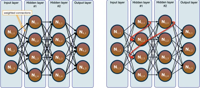
Input layer Hidden layer Output layer #2 Hidden layer #1 N1,3 N1,1 N1,2 N2,1 N2,2 N2,3 N2,4 N4,2 N4,3 N4,1 N3,1 N3,2 N3,3 N3,4 weighted connections Hidden layer #1 Hidden layer #2
Input layer Output layer
N1,3 N1,1 N1,2 N2,4 N4,2 N4,3 N4,1 N3,2 N3,3 N3,4 N3,1 N2,3 N2,2 N2,1
Figure 1.1: Examples of artificial NNs: (left panel) FFNNs and (right panel) RNNs. The first generation of NNs comprises of layers in which the output of a layer is fed as input to the subsequent one, and thus the information flows uniquely in one direction. This type of networks are called Feed Forward Neural Networks (FFNNs), an example of which is given in the left panel of Figure 1.1. Nowadays, perceptrons are considered being a subcategory of FFNNs, since they are algorithms for learning binary classifiers and characterized by having an input vector and a weight vector.
In order to adapt a network to a particular task, in fact, it has first to learn it. This is done by means of training procedures, which can be performed with different
approaches, such as supervised learning (i.e. expected values and obtained values
are compared, and this residual error is iteratively minimized) and reinforcement
learning (i.e. a learning agent sequentially selects actions, observes rewards, and
aims to maximize the total reward over a period of time). Since these two categories of learning processes interest the present project, more details about them are given in Chapter 3.
What makes the learning possible is that the output of the network changes if the weights of the connections are changed. Thus, the learning process consists of iteratively calculating (and reducing) an output error as a function of the weights of the connections. In more detail, each iteration corresponds an update of the synaptic weights following the so-calledgradient descent algorithm: steps along acost function
are taken in the direction towards which its gradient decreases. The cost (or loss, or objective) function for calculating the output error can be chosen among many possible functions, such as the Mean Squared Error (MSE) function and the cross-entropy error function, which was used for this project.
Another key-concept in artificial NNs is a function assigned to each node and that determines the extent with which the change of the network weights gives a change
in the output: it is the so-called transfer function of the neurons. This function
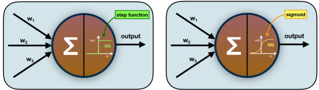
maps the input received by the neuron with the output it will generate. Originally, perceptrons were characterized by having a step function as transfer function, but what one ideally wants for a neural network is that small changes in the weights cause only small changes in the output, and such a non-continuous function was
not ideal. For this reason, a sigmoid function was introduced as neuronal transfer
Ʃ
w1 w2 w3 f(S) output step function in outƩ
w1 w2 w3 f(S) output sigmoid in outFigure 1.2: Perceptron (left) and sigmoid neuron (right). The weighted inputs are col-lected and an output is generated by means of a transfer function.
its smoothness (i.e. continuity) the sigmoid is commonly used in artificial NNs. In Figure 1.2 a schematic depiction of a perceptron and of a sigmoid neuron is given.
During the learning process, in order to compute the gradient of the cost function, the output error is first calculated and then distributed back through the network layers by means of the so-calledbackpropagation algorithm. In this way, the weight of each connection can be assessed and updated. When the cost function has reached a minimum, the training algorithm has succeeded. However, this procedure is not trivial, and it can present obstacles in many situations. For instance, for the hidden layers of a network, when their number increases, even if intuitively it would seem to enhance the potentiality of the network, it induces complications in the backprop-agation algorithm. In particular, it can mean either for the early layers to learn more slowly than the late ones, or vice versa. These phenomena are due to a
cer-tain instability of the gradient in deep networks and are known as vanishing- and
exploding-gradient problem, respectively. In order to control this aspect, it is possible
to choose a cost function and a transfer function, i.e. the function that describes
the output of a single node given the input received, which make the gradient less unstable[4, 5].
In general, the backpropagation algorithm can be used not only for FFNNs, but also when more complicated architectures are considered, such as networks with feed-back loops. These different patterns for the information flow in which neurons can send their output to neurons of previous, same, or subsequent layers are employed in the so-called Recurrent Neural Networks (RNNs)[6]. An example of RNNs can be seen in the right panel of Figure 1.1. These are considered a particularly important class of NNs, since they include the time dimension in the network, not contemplated in the standard architecture. In fact, by discretizing time in steps of fixed length, the RNNs can be trained to remember information and use it at a later point in time. Schematically, RNNs are represented as FFNNs with repeated weights and units (i.e. the recurrent ones), and that is why FFNNs can be seen as a special case of RNNs. However, these networks are very hard to train because an error has to be backpropagated in time. These difficulties derive from the fact that the derivative of the activation function of the same neuron needs to be applied for multiple time steps and, as mentioned earlier, the gradient in deep neural nets is not stable. This leads to an increased gradient instability for RNNs and, for this reason, while RNNs should theoretically be able to connect information even when the gap between the relevant information and the point where it is needed becomes very large, in practice that was found to be not true[7, 8].
Hidden layer #1
Hidden layer #2
Input layer Output layer
N1,3 N1,1 N1,2 N4,2 N4,3 N4,1 N3,2 N3,3 N3,4 N3,1 N2,3 N2,2 N2,1 LSTM
Input layer Hidden layer #1 Hidden layer #2 Output layer N4,2 N4,3 N4,1 N3,2 N3,3 N3,4 N3,1 LSTM N2,3 N2,2 N2,1 N1,3 N1,1 N1,2 output gate CEC input cell input gate forget gate output cell
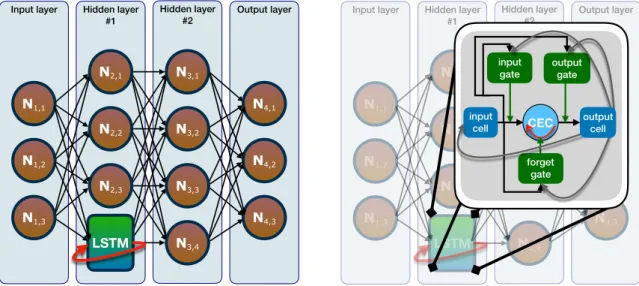
Figure 1.3: Examples of LSTM networks (left panel) and of LSTM units (right panel). Among the many types of RNNs, one of the most important and popular (and the one included in this project), uses a particular memory unit called Long Short-Term Memory (LSTM)[9], which, due to gating structures, avoids the just-mentioned learning problem for short-term memory, i.e. for which the representations of recent input events are stored in form of activations. An example of networks including such architecture is shown in the left panel of Figure 1.3.
1.1.1
Long Short-Term Memory architectures
As anticipated earlier in this chapter, RNNs present a problem in using backpropa-gation. In fact, the backpropagated error over time depends exponentially on the size of the weights, leading to exploding and vanishing gradient issues. For this reason, it was necessary to come up with an architecture designed to overcome these obstacles hampering the training procedure.
LSTM is an architecture that allows the incorporation of memory in a network and, in particular, to handle the learning of long-term dependencies[9]. It consists of a group of neurons having different behaviors, namely a memory cell which (1) preserves its state over time, hence making it possible for information to persist, and (2) allows constant error flows (i.e. the activation function is an identity function, hence the derivative is always equal to one, hence it does not affect the backpropagation), and gates which control the information flow into and out of the memory cell. Thanks to this structure and in particular to the design of the memory cell, which is the central feature of LSTM and called Constant Error Carousel (CEC), the aforementioned errors can be avoided. Different behaviors are obtained by tuning some parameters. In particular, to make a neuron behave like a gate, it is important to assign it an appropriate transfer function, which has been a crucial point of attention in the course of the present project.
Many variants of the original LSTM unit exist. The most popular are composed of three gating units (input, forget, and output, which control the information flowing into, persisting in, and exiting from the LSTM, respectively), a CEC, and an output activation function[10], as shown in the right panel of Figure 1.3. The forget gate, in particular, by discarding non-relevant and previously stored information (i.e. the
new state of the CEC is obtained by multiplying the previous state by a factor∈[0,1] which depends on the information flowing from the input cell to the forget gate), is a key feature of LSTM for continually running networks.
1.1.2
Spiking Neural Networks
The idea of artificial NNs finds its roots in one of the most efficient learning and control system known: the brain. In fact, since its neuronal activity mostly depends on the extent with which the input changes, the information flow in the brain is characterized by a sparse nature[11], which translates into energy efficiency.
However, with time the link between biological and artificial NNs has become increasingly tenuous. Nowadays, the related scientific research is mainly oriented towards finding NNs which give higher efficiency and are easy to implement[12]. Nevertheless, scientists have recently started to consider the idea of using networks based on mathematical models of the brain with the goal to achieve its level of efficiency, i.e. the SNNs[13, 14].
In 1952 the first scientific model of a spiking neuron was proposed by Hodgkin and Huxley[15], based on experiments performed on the giant axon of the squid.
They succeeded in measuring the currents leading to action potentials, i.e. the
prop-agating change in membrane potential controlling the neuronal dynamics, and their mathematical model constitutes the basis for a very detailed neuronal description. Other models (some of which are presented in the next section) were subsequently developed by reducing the amount of details in order to increase the computational efficiency and implementation of the networks, and thus to favor their use in Machine Learning tasks.
Relying on this idea of action potential propagation for passing information be-tween nodes, SNNs are networks in which the neurons, instead of constantly
commu-nicating the same piece of information, send each other spikes of signals, i.e. small
electrical pulses (the biological ones have amplitude of 100 mV and duration 1-2 ms) corresponding to the propagation of action potentials, at either regular or irregular in-tervals, separated by at least a minimal distance referred to as theabsolute refractory period of the neuron1. Once the spike train is received, it can cause a change in the
membrane potential, i.e. a quantity that simulates the potential difference between
the interior of the biological neuron and its surroundings, of the next neuron. At this point, if the potential of the receiving neuron reaches a critical value above theresting
potential, i.e. the value of the membrane potential when no inputs were received for
some time (approximately −65 mV), this neuron, in turn, starts generating spikes.
The critical voltage for spike initiation is commonly described by a threshold ϑ, and
the moment of threshold crossing defines the firing- or spike-time. In Figure 1.4 a
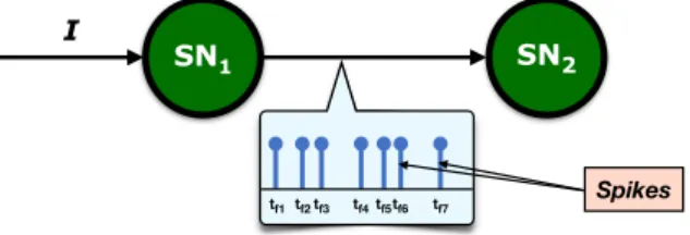
schematic representation of the functioning of two spiking neurons is given.
The neuron sending spikes can thus be seen as an encoder of information, which then has to be decoded by the receiving neuron. In these regards, it is important where, in the context of this spike-mechanism picture, the biggest amount of informa-tion resides. The shape of the pulse does not change while it propagates, and different isolated spikes have the same shape, hence the form cannot be used to retrieve the
1http:// www.physiologyweb.com/ lecture notes/ neuronal action potential/ neuronal action potential refractory periods.html
I
SN1 SN2
tf1tf2tf3 tf4tf5tf6 tf7 Spikes
Figure 1.4: Depiction of spiking neurons and their characteristic event-based coding. encoded information. Instead, other information holders have been studied, such as the firing rate, i.e. the number of spikes per time interval reaching the subsequent
neuron (rate coding[16]), or the spike time, which gives to the information flow in
SNNs an event-based nature (temporal or spike-time coding[17]).
The spiking nature of these neurons gives rise to a fundamental problem in the implementation, since the spikes are not differentiable, thus hampering the training and backpropagation processes (that can usually be performed due to the differentia-bility of each component of the networks). Training algorithms for spiking networks have been studied, but they are much less efficient than the training procedure for the standard artificial networks. A solution to this issue–and the one implemented in the present work–is to use analog neurons for training and subsequently replacing them with spiking neurons, with the condition that the activation function of the analog neurons has to approximate the behavior of the spiking neuron.
1.2
Spiking Neural Networks and Physics
There are many links between Physics and artificial NNs, for example in the last few decades models for NNs based on Quantum Mechanics have been studied. These nets, known as Quantum Neural Networks (QNNs), are built using the principles of quantum information processing, which translates into taking into account not only the amplitude but also the phase of the signal[18]. The ongoing research focuses on exploiting the computational and statistical complexity provided by quantum perceptron models[19]. The ability of QNNs in image compression was tested and it was found that their efficiency was comparable if not greater than standard neural nets[20].
In the same way QNNs can be seen as the point of contact between Quantum Mechanics and Deep Learning, SNNs are the meeting point between Biophysics and Deep Learning. More in general, Physics and SNNs are interlinked with each other, since the former is deeply embedded in the theory underlying the spiking neural models and the implementation of SNNs for data gathering, storage, and analysis could lead to higher efficiency time- and computational-wise, useful in many branches of Physics research.
1.2.1
Biophysics of the Spiking Neural Model
In Physics, one has to distinguish between different scales, for which distinct
mathe-matical formulations hold, e.g. the very Newton’s second law, F =ma, is very
effi-cient in describing systems at big scales but, when going down to small (i.e. atomic) scales, it does not hold anymore, and that is when a different formalism, i.e. quantum
mechanics, comes to the rescue. In the same way, different biophysical models for the neuron exist, which can be classified depending on both the amount of details included and the computational efficiency of their implementation. In particular, the very foundation of all the spiking neural models developed so far comes from concepts borrowed from Physics, and thus they can be seen as different physical models. In this section some models are presented, going from the best in terms of completeness and amount of details included, through more simplified phenomenological ones, to the most efficient when it comes to implementation.
Hodgkin-Huxley
The most detailed description of neuronal dynamics is given by the Hodgkin-Huxley model[15], as mentioned in the previous section. It can characterize in detail different types of synapses and the spatial geometry of each neuron by means of a set of differential equations describing the dynamics of the currents flowing through the semipermeable cell membrane via ionic channels, leading to action potentials. The entire neuronal dynamics, in fact, stems from electrical potentials generated by a difference in ion concentrations between the inside of the neuron and the surrounding environment.
In principle, a complete biophysical model for the neuron can be built if both the channels present and their respective parameters are known. Originally, Hodgkin and Huxley included in their theory only two ionic channels, i.e. sodium and potas-sium, and a leakage channel. Under this assumption, the Hodgkin-Huxley model is represented by a system of four nonlinear differential equations:
I(t) = Cdu dt +gNam 3h(u−E Na) +gKn4(u−EK) +gL(u−ELL), ˙ m=− 1 τm(u) [m−m0(u)], ˙ n=− 1 τn(u) [n−n0(u)], ˙ h=− 1 τh(u) [h−h0(u)]. (1.1)
The first equation describes the current at the level of the membrane. It is composed of a contribution representing the charging current and three terms representing the current flowing through the ion channels (the subscript L refers to unspecific leakage
channels), regulated by some gates. The parameter gi and the quantity Ei are,
respectively, the conductance and the voltage relative to the channel i. The other
three equations are the evolution of the gating variables m, n, and h, with m and h
controlling the evolution of the sodium channels, and the gating variable n controls
the potassium channels. A more detailed procedure leading to System 1.1 is given in the Appendix.
This model can describe many processes part of the neuronal dynamics. For example, if immediately after a spike another input is delivered to the
Hodgkin-Huxley model, evidence of refractoriness can be observed. This is due to a lowering
the gap between the value of the membrane potential and the critical point is bigger than the initial value. The intrinsic refractoriness of the neuronal signal represents a crucial feature in spike-based communication that needs to be taken into account when using adapting spiking networks, and it will thus be mentioned again in the course of this thesis.
Even though their description is outside the scope of the present work, it must be mentioned that many other neuronal dynamics aspects can be correctly described by the Hodgkin-Huxley model. However, despite its accuracy and robustness, the difficulty in visualizing and analyzing the behavior of high-dimensional systems of non-differential equations it is not insubstantial. For this reason, a reduction to two dimensions can be conveniently studied, since for systems of two differential equations a mathematical analysis is possible.
FitzHugh-Nagumo
The first proposing to study the generation of action potentials by reducing the dimensions of the neuronal model from four to two were FitzHugh and Nagumo[21, 22]. By applying some approximations (for more details, see the Appendix), the neuronal dynamics can be described by the following two differential equations:
du dt = 1 τ[F(u, w) +RI], dw dt = 1 τw G(u, w), (1.2)
with R being the resistance and some functions F and G, such that G interpolates
between dn/dt and dh/dt.
Following this path, different mathematical formulations for the functions F and
G were proposed. FitzHugh and Nagumo defined them as
F(u, w) = u− 1
3u
3−w ,
G(u, w) = b0+b1u−w ,
(1.3)
obtaining sharp pulse-like oscillations reminiscent of action potentials.
In order to visualize the temporal evolution of the variables (u, w) the
two-dimensional phase plane analysis can be used. The neuron, in fact, being a system that evolves over time, can be considered as a dynamical system. By integrating the Equations 1.2 over time, the evolution of the state of the system (i.e. the neuron) can be studied. By performing such a study, the presence of three fixed points in the phase portrait of the FitzHugh-Nagumo model can be highlighted, due to
in-tersections of the u- and w-nullclines (i.e. the points such as ˙u = 0 and ˙w = 0,
respectively). By solving an eigenvalue problem, the study of the stability of these
points can be performed. Hence, by means of the Poincar´e-Bendixson theorem, the
existence of a limit cycle can be proven, leading to the interpretation of the neuron as an oscillatory system: following the trajectories obtainable by injecting a positive
I into the system, the voltage follows rapid changes, which can be seen as a train of
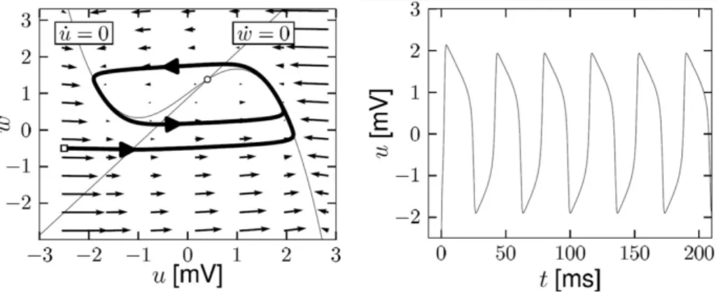
spikes. In Figure 1.5 the nullclines and the trajectory, i.e. a limit cycle (resulting from the integration over time of a dimensionless version of Equations 1.2, see [23] for
Figure 1.5: Phase plane analysis for the FitzHugh-Nagumo model with dimensionless variables. Left panel: nullclines for I=2 and trajectory (thick line); right panel: voltage time course along the trajectory shown in the left panel.[23]
further details), of the FitzHugh-Nagumo model for a positive input are shown (left panel), together with the voltage time course of the trajectory (right panel), showing a spiking trend.
Leaky Integrate-and-Fire (LIF)
The integrate-and-fire family of models can be interpreted as the opposite of the Hodgkin-Huxley model, since they are stripped of all the biology inspired details and very easily implementable, thereby representing the most basic neuronal models. The simplest version of the Leaky Integrate-and-Fire (LIF)[24, 25, 26, 27] model is constituted of a single linear differential equation describing the evolution of the membrane potential and a threshold for spike firing.
The name derives from the fact that, as a first approximation, the dynamics of neurons can be described as a summation (or integration) process. In fact, for low firing rates the total change of potential in the postsynaptic neuron is given by the summation of the changes of potential caused by each individual presynaptic neuron. In a slightly more general version of this model (i.e. the nonlinear LIF), when the potential u crosses the threshold ϑreset, a spike is generated, defining the firing time
tf, and, instead of having a relaxation variable like in the previous models, here the membrane is reset after every spike.
However, neglecting the more detailed cases (not covered here) in which the phe-nomenon of adaptation is included in the picture, the linear LIF model can be rep-resented by an ensemble of discrete physical components: a capacitor and a resistor placed in parallel and driven by a current. In particular, the membrane is seen as a ca-pacitor with a finite leak resistance. By means of the law of current conservation, the input current I(t) is split in two components: a resistive current IR = [u(t)−urest]/R
and a current IC = dq/dt=Cdu/dt that charges the capacitor, giving the following:
I(t) =IR+IC
= u(t)−urest
R +C
du
dt , (1.4)
is obtained:
τm
du
dt =−[u(t)−urest] +RI(t), (1.5)
which is a linear differential equation describing a RC-circuit with the resistor and the
capacitor arranged in parallel, or equation of a passive membrane. The solution
as-suming that fort >0 the input vanishes and with initial conditionu(t0) = urest+ ∆u
is given by[23]: u(t)−urest= ∆uexp −t−t0 τm fort > t0. (1.6)
This shows that with no input the membrane relaxes back with a decay regulated by
τm (usually equal to approximately 10 ms) to the resting value. In this framework,
ϑreset can be interpreted as the minimal voltage necessary to cause a spike.
This one-dimensional model is being used for doing simple computation with SNNs but, since it does not take into account of adaptation, it is considered oversimplified in the sense that it cannot describe the firing mechanism of biological neurons at all, in contrast to the rest of the previously-presented models.
Spike Response Model (SRM)
Another mathematical description of neuronal activity, and the one underlying the model used in thesis, is given by the so-called Spike Response Model (SRM)[28, 29]. It can be derived from the LIF by integrating a series expansion[14], however it differs from the other models presented in this section because, instead of making the variables changing as a function of the voltage, here they are described by the spike time and in particular by the time passed since the last output spike. The SRM simplifies the spike generation mechanism while keeping a very rich description in terms of neuronal refractoriness and adaptation. In fact, the firing of a spike at time
t is obtained whenever the membrane potential reaches–from below–the threshold
ϑ(t), which is time-dependent, or, in formula:
t =tf ⇔ u(t) = ϑ(t) and
d[u(t)−θ(t)]
dt >0, (1.7)
with tf as the firing time.
In this framework, the variable u describing the membrane potential fully
char-acterizes the state of the neuron and its evolution over time is given by:
u(t) = Z ∞ 0 η(s)S(t−s)ds+ Z ∞ 0 κ(s)Iext(t−s)ds+urest, (1.8)
withIext(t) representing an external time-varying stimulating current,urestthe resting
potential, S(t) the spike train,κ andη being two kernels controlling the shape of the membrane and of the voltage-dependent output, respectively. More in detail, the membrane shows a linear response to an injected current, and, on the other hand,
it takes time for the membrane to decay back to the value of urest after receiving an
input. The two filters κ and η respectively control these two processes.
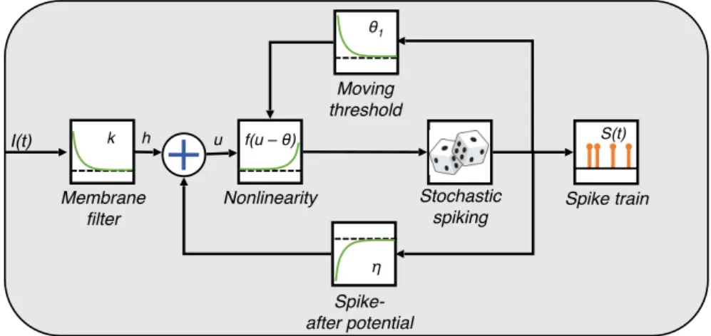
It was proved that, if some features are added to a more detailed version of this model, the in-vitro experimental signal made of spikes can be fitted with a precision in the order of milliseconds[30]. In Figure 1.6 a depiction of the SRM including adaptation is shown.
I(t) h u S(t) Membrane filter Nonlinearity Stochastic spiking Moving threshold Spike-after potential Spike train f(u – θ) θ1 η k
Figure 1.6: Schematic description of the SRM. The variablehindicates the input potential after being filtered; the other quantities are presented in the text.
1.2.2
Applications in Physics
From gene mapping to space exploration, the problem of gathering data sets so huge that are difficult to save and analyze concerns many disciplines, as described by Sivarajah et al.[31].
Thanks to a better balance between communication time and computation cost than traditional networks, SNNs have demonstrated great potential in big data analysis[32]. Many applications use RNNs to integrate or store signals through time, but the standard NN computation lacks the natural notion of time (i.e. it is a frame-based method), which makes this approach not appropriate, whilst, on the other hand, SNN computation is time-based. These networks carry advantages particularly tied to parallel computing, a type of computation which has been used to model problems, on top of other scientific domains, in many branches of Physics, such as applied, nu-clear, particle, condensed matter, high pressure, fusion, and Photonics[33, 34, 35, 36]. Astrophysical observations, for example, involve the gathering of huge amounts of data[37]. Machine Learning techniques have been already giving major support to this type of applications[38] by effectively building a priori knowledge that can be used to go beyond the deconvolution limit set by the Shannon-Nyquist sampling criterion[39]. A further and more specific example is given by the research conducted at the Large Hadron Collider (LHC)[40] facility, where the Higgs boson was discovered. On July 4, 2012, after collecting and analyzing 500 trillion proton collisions[41], the existence of a boson of mass could be announced. This figure is a prime example of the extent of the necessity for scientists, which typically have to select images showing some desired features and discard the rest, i.e. a practice requiring a lot of manual tuning, to find more efficient solutions for data gathering, storing, and processing. In particular, with regard to the issue of data storage, in 2005 the world’s first petabyte-sized database was introduced with the BaBar experiment[42]. Because of some limitations found at that time, however, it was decided to store data in ROOT and that is how today hundreds of petabytes of data worldwide are stored, even though ROOT has been criticized for many aspects, such as the difficulty for beginners, its design,
and its implementation2. The same issues interest other branches, and in particular
it applies to X-ray Crystallography, a technique for determining three-dimensional
atomic structures through light-scattering detection. Besides the problem of data storage, for these experiments, in order to recognize the presence of Bragg peaks in images, multiple offline analyses months after the experiment are usually needed to be completed[43]. In these regards, the attractiveness of in-situ fast data storage and analysis offered by SNNs stands out.
Moreover, given the asynchronous nature of spiking LSTM, the implementation of SNNs would bring a major benefit to additional research fields for which the estimation of the correlation between time series is required. Experiments involving the practice of collecting data at different frequencies is, in fact, hampered by the
use of a time window by the detectors. Spiking LSTM networks would provide
asynchronous data gathering, allowing simple signal decorrelation. This feature would be beneficial also within other fields, such as medical and financial applications [44], but of course scientific research in general would receive a boost from asynchronous detection and computing. An example of the procedures which would take advantage of the implementation of spiking memory networks is given by LIght Detection And Ranging (LIDAR), a remote sensing technique used to probe objects at various scales at very distant positions by detecting the backscattered radiation of pulsed lasers. Distances are thus found by calculating the time span between the moment at which the pulse was sent and the detection time, hence a detection without an internal clock would allow to greatly improve these measurements.
The introduction to SNNs as new computing architectures for handling big data and time series is so promising that a relatively new research branch known as Neuromorphics[45, 46] has been sprouting. Its main goal is to develop chips able to process data the same way our minds do, and, by incorporating these chips into detectors, every imaging facility would benefit of the possibility of computationally efficient in-situ exploration. As Paolo Calafiura (software & computing manager for the LHC ATLAS experiment) said: ”The field of neuromorphic computing is very new, so it is hard to say conclusively whether science will benefit from it. But from a particle physics perspective, the idea of a tiny processing unit that is self-contained and infinitely replicable is very exciting”.
In these regards, many neuromorphic studies have been emerging. In 2014, the American multinational technology company IBM developed and produced the first neuromorphic chip, called TrueNorth[47], and in 2016 IBM scientists published a paper proving that convolutional networks could run quickly and accurately on said neuromorphic chip[48]. In 2014 the Advanced Processor Technologies Research Group (APT) at the School of Computer Science, University of Manchester, designed a
com-puter architecture named SpiNNaker (Spiking Neural Network Architecture), which is
planned to be a massively parallel computing platform based on SNNs [49]. Moreover, earlier this year Intel announced a neuromorphic artificial intelligence test chip named
Loihi3, which will be produced in the next few months. The curiosity arising withing
the scientific community towards SNNs can be also noticed from the fact that, cur-rently, scientists at Berkley have been testing whether these brain-like architectures have the potential to handle Big Data problems. On a final note, a spiking LSTM net-works was implemented by TrueNorth[50], however it does not provide asynchronous data processing, resulting in a less-efficient and less biologically plausible model than the one proposed in this thesis.
The model
As stated previously, the scope of this project is to study a model for spiking neurons which could be applied to LSTM networks, in order to exploit the potential of SNNs and make a small step towards their implementation in many scientific branches. The main goal is to study and optimize the conversion from analog to spiking neurons, to obtain spiking working memory networks.
In this chapter, at first, the neuronal model used for modeling the behavior of the spiking neurons involved is described. Subsequently, the problem of finding a transfer function for the analog neurons in order for them to be able to describe how their spiking counterparts communicate information is addressed, with the goal of training the LSTM network using a continuous and derivable function. Specifically, an analytical solution biologically plausible is firstly derived mathematically, in order to study whether this option could bring some advantages, e.g. error reduction, in the storing process of the memory cell of the LSTM units, i.e. the CECs (analyzed in the next chapter). Successively, the procedure leading to another solution (which will be tested in the next chapter) is presented, involving the incorporation of a stochas-tic behavior in the neuronal model initially described. Finally, since the Machine Learning tasks were used to test only the stochastic network, the adaptive stochastic LSTM unit is presented at the end of this chapter, followed by an overview concern-ing the theory of the learnconcern-ing algorithms involved in this thesis (i.e. supervised and reinforcement learning).
2.1
Adaptive Spiking Neurons
The spiking neurons that were used for this project are multiplicative Adaptive Spik-ing Neurons (ASNs) as described in [51] and their analog counterparts, Analog Adap-tive Neurons (AANs). This neuronal model is a variant of an adapting SRM that includes fast–multiplicative, instead of additive[52, 53]–adaptation to the dynamic range of input signals, i.e. a central characteristic for obtaining efficient neural cod-ing.
The adaptation is included in two senses: by considering (1) spike-triggered adap-tation currents and (2) a dynamical threshold, leading to an increased gap that has to be filled in order for a neuron to emit a spike, thus giving even sparser signals i.e.
more computational gain. This multiplicative version was proven to be able to main-tain a high coding efficiency for inputs that vary over several orders of magnitude, unlike its additive counterpart, while still matching neural responses[51].
More in detail, the behavior of the just-introduced ASNs is mathematically
de-scribed by the following equations[51, 54], expressing the incoming signal (i.e.
in-coming postsynaptic current), the effective received signal, filtered by the neuron (i.e.
input signal), the dynamical threshold determining the critical value the potential
difference has to reach for meeting the spike-firing condition, and the internal state
of the neuron:
incoming postsynaptic current: I(t) = X
i X tf i wiexp tf i−t τβ , (2.1) input signal: S(t) = (φ∗I)(t), (2.2) threshold: ϑ(t) = ϑ0+ X tf mfϑ(tf) exp tf −t τγ , (2.3) internal state: Sˆ(t) = X tf ϑ(tf) exp tf −t τη , (2.4)
where wi is the weight (synaptic strength) of the neuronal incoming connection,
tf i < t denote the spike times of the presynaptic neuron i, and tf < t denote the
spike times of the neuron itself, φ(t) = φ0exp(−t/τφ) is an exponential smoothing filter with time constant τφ, ϑ0 is the resting threshold, mf is the multiplicative variable controlling the speed of spike-rate adaptation, and τβ, τγ, and τη are the time constants that determine the rate of decay of I(t), ϑ(t), and ˆS(t) respectively. The neural coding process can then be seen as a sigma-delta modulation[55] (i.e. an encoding process of analog signals into digital signals) for which the receiving neuron decodes the information encoded by the previous neuron by using as starting point the exact times of the spikes.
For this neuronal model, for an ASN receiving a constant input S, the neuron fires a spike whenever:
S−Sˆ(t)>0.5·ϑ(t), (2.5)
which can be biologically interpreted as the point at which the different between the outer (S) and the inner ( ˆS) potential of a neuron reaches a critical limit, set as half
the value assumed by the membrane potential (ϑ) at that specific moment.
Hence, for our artificial spiking neurons, whenever the spike-firing condition (which was defined in [51]) is met, three things happen: (1) the neuron emits a spike of fixed
height h (which, as suggested by [56], is set to the value h = 1) to the synapses
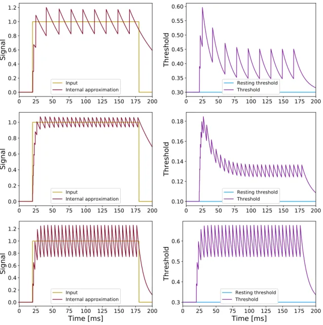
connecting to the target neurons, (2) a value equal to ϑ(tf) is added to the internal state ˆS, withtf the spike time, and (3) the threshold is increased by a valuemfϑ(tf). Some examples of these adaptation processes are depicted in Figure 2.1, with the red (left column) and the purple (right column) curves showing, respectively, how the internal approximation ˆS(t) and the threshold ϑ(t) vary over time when a constant input current is injected into an ASN, for different sets of values of certain parameters of the neuron; in the first row, the plots were obtained by setting biologically plausible
0 25 50 75 100 125 150 175 200 0.0 0.2 0.4 0.6 0.8 1.0 1.2
Sig
na
l
Input Internal approximation 0 25 50 75 100 125 150 175 200 0.30 0.35 0.40 0.45 0.50 0.55 0.60 Th re sh ol d Resting threshold Threshold 0 25 50 75 100 125 150 175 200 0.0 0.2 0.4 0.6 0.8 1.0Sig
na
l
Input Internal approximation 0 25 50 75 100 125 150 175 200 0.10 0.12 0.14 0.16 0.18 Th re sh ol d Resting threshold Threshold 0 25 50 75 100 125 150 175 200Time [ms]
0.0 0.2 0.4 0.6 0.8 1.0 1.2Sig
na
l
Input Internal approximation 0 25 50 75 100 125 150 175 200Time [ms]
0.3 0.4 0.5 0.6Th
resh
old
Resting threshold ThresholdFigure 2.1: Examples of adaptation dynamics for the ASNs. The internal state together with the input current (left column) and the threshold together with the resting threshold (right column) are plotted as functions of time for different values of some of the neuronal parameters: (top panels) τη = 50ms, τγ = 15ms,ϑ0 =mf = 0.3; (middle panels)τη = 50 ms,τγ= 15ms,ϑ0 =mf = 0.1; (bottom panels) τη =τγ = 10ms,ϑ0=mf = 0.3.
threshold and multiplicative factor ϑ0 = mf = 0.3; in the second row of plots the
threshold and multiplicative factor were changed toϑ0 =mf = 0.1, while the last row
represents very fast neuronal adaptation dynamics, obtained by setting τη =τγ = 10
ms while keeping the original values of ϑ0 = mf = 0.3. For all the curves, the
first few spikes happen very close to each other. This is the transient phase of the
neuron, i.e. the phase during which the neuron adapts to the signal before getting stable after being silent for some time, and it could represents a source of error when spiking neurons are switched with analog neurons. The signal that needs to be communicated by the neuron is in fact the part of the signal after the transient phase. Precisely, the spikes fired during the transient phase can cause a sudden increase in the signal when perceived by the next neuron, and this is one of the major problems
Ʃ
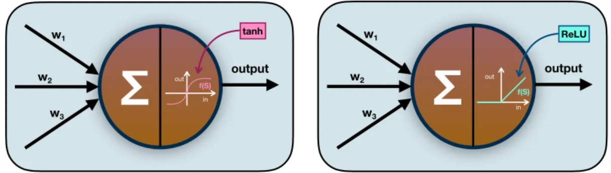
w1 w2 w3 f(S) output tanh in outƩ
w1 w2 w3 f(S) output ReLU in outFigure 2.2: Tanh (left) and ReLU (right) neuron. The weighted inputs are collected and a different output is generated depending on the choice of the transfer function.
encountered, e.g., in the LSTM conversion used in this project, as it will be shown in Chapter 4.
Overall, still by looking at the plots in Figure 2.1, it is noticeable that by reducing the resting threshold and the multiplicative factor at the same time (i.e. going from the first to the second row of plots), the variance of the signals decreases but the firing rate increases (i.e. the spikes are less sparse), whilst the trend of the adaptation does not change, giving overall a more precise signal encoding. Instead, by decreasing the time constants (i.e. compare the first and the third rows of plots) the speed of the adaptation changes, specifically the adaptation happens quickly leading to an increase in the firing rate. It must be mentioned that, in the present study,τβ (i.e. the time constant regulating the decay of the incoming postsynaptic current) is always considered to have the same value as τη (i.e. the decay constant of the internal state of the neuron), in order to allow for the neuron receiving the signal to be able to decode the signal sent from the previous neuron. The trends depicted in the figure represent some examples of how it is possible to tune the behavior of the spiking neurons by changing the values of the parameters in the neuronal model.
2.2
Transfer function
As mentioned in the previous chapter, the function that maps the input signalSto the
average Post Synaptic Current (PSC)Ithat is perceived by the next (spiking) neuron
is known as transfer function. Thus, even if in the present thesis a neural coding approach based on spike-time coding is used, the concept of transfer function stems from a rate-coding approach. Originally, in fact, based on a rate-code interpretation,
the firing rate of the neuron was modeled with an activation function f(S), which
represented the frequency of the spikes along the axon, and the transfer function used for NNs was then the sigmoid functionf(S) = 1+1e−S, which is symmetric about 0.5 and has two horizontal asymptotes (in 1 and 0, respectively). However, since no negative activations are allowed by using the sigmoid, the hyperbolic tangent (tanh), i.e. a particular case of sigmoid function symmetric about zero, was considered. A very different variation of the sigmoid neuron is given by the Rectified Linear Unit
(ReLU), expressed as f(S) = max(0, S), which, thanks to the convenient gradient,
when chosen leads to easily trainable networks. In Figure 2.2 a tanh neuron and a ReLU neuron are displayed (compare with Figure 1.2 in the Introduction).
it-eratively updating the synaptic weights by means of the backpropagation algorithm, during which the derivative of the transfer function is computed at the level of each individual neuron. For this reason, a network needs to be made of differentiable com-ponents in order to be trained through backpropagation, and a function which has derivative equal to 1 such as the ReLU makes it easier for the training procedure to update the weights. In the past, the use of ReLU was the solution to the vanishing gradient problem, for which the gradients assume increasingly smaller values, ham-pering thus the learning process. For the gating mechanisms typical of LSTM units, however, the ReLU is not a good candidate, because such a linear shape is not able to describe the gating behavior. For the gates, in fact, saturation (i.e. the presence of horizontal asymptotes) is necessary: a gate should ideally be either completely open (i.e. asymptote in 1) or completely closed (i.e. asymptote in 0).
For this project, the training procedure was chosen to be performed on analog neurons (because spike-based learning is slow and poorly effective), and then, once the training process ends (i.e. once the weights of the connections were set such as an error is minimized), the analog units were switched with spiking units while keeping the weights fixed, and the obtained spiking networks were used to perform the tasks. In order for this approach to be valid, the problem of finding an errorless superposition between the behavior of analog and spiking neurons has to be addressed. Here, it was decided to base this superposition on the neuronal transfer function, which translates into looking for a mathematical expression of the spiking transfer function. In fact, by applying such mathematical expression as transfer function for the analog neurons, the single units (analog and spiking) would process inputs in the same way, guaranteeing thus the possibility to train the analog networks off-line and take advantage of the state-of-the-art techniques in Deep Learning, being sure then when the analog nodes are switched with spiking nodes the network would solve the tasks it was trained to solve. In Figure 2.3 a schematic depiction of the analog/spiking conversion can be found.
An analytical transfer function describing the activation of spiking neurons was
already exactly derived for the case τβ = τη = τγ and approximated for the case
τβ = τη 6= τγ by considering a constant current input and equilibrium values for ϑ, ˆ
S, and I. For completeness the mathematical procedure leading to such functions is
shown in the Appendix.
However, when testing the obtained transfer function on a simple network of three neurons (i.e. one input, a CEC, and one output) an offset between the update of the analog and the spiking CEC was noticed[57]. This error would lead to a mismatch be-tween how the analog neurons are trained and the spiking neurons perform the tasks. Moreover, the results of the same study reported high firing rates which, together with some specific features of the LSTM architecture designed back then (which will be described later in this chapter), lead to, overall, low biological plausibility for the system. These are the reasons why it was decided to try the implementation of a stochastic adaptive spiking neuron in the first place.
Therefore, in order to obtain a better neuronal model, two new transfer functions are derived and tested in this project: an analytical solution, i.e. a variation from the original study, for a different ratio between τη and τγ (specifically, τη = 2τγ, which reflects more the relationship between the biological values of these time constants), and a transfer function describing the stochastic behavior of the neurons.
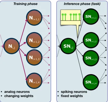
Training phase • analog neurons • changing weights Ni+1,2 Ni+1,1 Ni+1,3 Ni+1,4 Ni,j
Inference phase (task)
• spiking neurons • fixed weights SNi+1,2 SNi,j SNi+1,1 SNi+1,3 SNi+1,4
Figure 2.3: Analog/spiking conversion. Left panel: training phase, the nodes are analog neurons and the weights are iteratively updated; right panel: inference phase, the analog nodes are switched with spiking units, the weights obtained at the end of the training process are now kept fixed.
2.2.1
Analytical solution
As previously mentioned during the discussion of Figure 2.1, typical values for the time constants τη and τγ are not on a ratio 1:1. Specifically, the decay of the internal state over time is usually much slower than the decay of the threshold. For this reason, when wondering which other function can be tested as transfer function, it would be useful to have the analytical solution for a situation in which there is a different ratio between the two time constants.
In order to find the analytical solution forτη = 2τγ, the assumptions and the first part of the procedure shown in Appendix A are used, for which the transfer function
f(S) is given by the average value of I(t). Thus, the following proceeding will have as a goal to express the average I(t) as a function of the inputS while including also the condition τη = 2τγ.
The starting point consists of noticing that, since the variables of the ASN decay exponentially (with time constants τβ, τη, and τγ), they converge asymptotically. Under the assumption of a constant input, a steady-state situation can be considered. Hence, at any spike time tf, I, ϑ and ˆS reach always the same value:
I(tf) =: If, (2.6)
ϑ(tf) =: ϑf, (2.7)
ˆ
S(tf) =:Sf, (2.8)
before being incremented by an amount equal toh, mfϑ(tf), andϑ(tf), respectively.
By setting τβ = τη (because of the reason expressed in Section 2.1) and t = 0 at
0< t < tf, as a function of these new quantities: I(t) = (If +h)e −τηt , (2.9) ϑ(t) =ϑ0+ (ϑf −ϑ0+mfϑf)e − t τγ , (2.10) ˆ S(t) = ( ˆSf +ϑf)e − t τη . (2.11)
By assuming that the Inter-Spike Interval (ISI), which is the time distance between two consecutive spikes, is constant, the next time a spike is fired can be set asts := ISI, hence at t=ts the following conditions are obtained:
I(ts) =If, (2.12)
ϑ(ts) = ϑf, (2.13)
ˆ
S(ts) =Sf, (2.14)
and the condition of firing translates then into the limit S−Sˆf = 0.5·ϑf.
Firstly, an expression for the transfer function can be derived from Equation 2.9 and Equation 2.12: f(S) = I(t) ts 0 = Z ts 0 (If +h)e − t τη dt· 1 ts =−τη ts (If +h) e−τηts −1 = h·τη ts , (2.15)
thus, an expression for ts as a function ofS is needed. It can be obtained by solving the system built by putting together Equation 2.10 and 2.13, Equation 2.11 and 2.14, and the limit of the firing condition:
ϑ0+ (ϑf −ϑ0 +mfϑf)e −τγts =ϑf, ( ˆSf +ϑf)e −τηts = ˆSf , S−Sˆf = 0.5·ϑf, (2.16)
which can be solved for the limit quantities, giving:
ϑf =ϑ0 1−e−τγts 1−(mf + 1)e −ts τγ , ˆ Sf =− ϑfe −τηts 1−e−τηts , ˆ Sf =S−0.5·ϑf . (2.17)
Furthermore, by plugging the last equation of System 2.17 in the second last equation, and by solving for ϑf, it leads to the following equation:
2S(1−e−τηts) 1−2e−τηts =ϑ0 1−e−τγts 1−(mf + 1)e −ts τγ , (2.18)
which can be further solved, thus giving, eventually: (2S+ϑ0)e −τηts −[2S(mf+1)+ϑ0]e −tsτγ1 +τη1 +[2S(mf+1)−ϑ0]e −τγts = 2S−ϑ0. (2.19)
From here, the original approach assumed the condition τγ = τη, whilst for the
present study the condition τγ =τη/2 is applied instead. By first making this substi-tution and then using x=e−τηts, the following steps can be made:
(2S+ϑ0)e −τηts −[2S(mf + 1) +ϑ0]e −3τηts + [2S(mf + 1)−ϑ0]e −2τηts = 2S−ϑ0 (2S+ϑ0)x−[2S(mf + 1) +ϑ0]x3+ [2S(mf + 1)−ϑ0]x2 = 2S−ϑ0 [2S(mf + 1) +ϑ0]x3−[2S(mf + 1) +ϑ0]x2+ 2ϑ0x2−2ϑ0x−(2S−ϑ0)x + 2S−ϑ0 = 0 [2S(mf + 1) +ϑ0]x2(x−1) + 2ϑ0x(x−1)−(2S−ϑ0)(x−1) = 0 [2S(mf + 1) +ϑ0]x2+ 2ϑ0x−2S+ϑ0 = 0
which eventually lead to the solutions:
x=e−τηts = −ϑ0± p 4S2−2Sϑ 0mf 2S(mf + 1) +ϑ0 . (2.20)
Of the two solutions, only the one with the plus sign is acceptable, since the other would give a negative argument for the logarithm. Thus, an expression for tsis found to be ts =−τηln " −ϑ0+p4S2−2Sϑ0m f 2S(mf + 1) +ϑ0 # , (2.21)
and, even if the intermediate steps are not reported here, it can then be plugged into the previously derived expression for the transfer function, i.e. Equation 2.15, obtaining: f(S) = h·τη ts = −h ln −ϑ0+√4S2−2Sϑ 0mf 2S(mf+1)+ϑ0 , (2.22)
in order to normalize the output of the analog neurons.
While his kept equal to 1 in the spiking neurons, for the analog neurons it needs
to be used as normalization factor, i.e. it can be set equal to the inverse of the limit for S → ∞ of f(S): h= 1 limS→∞f(S) = 11 ln 1 mf+1 = ln 1 mf + 1 . (2.23)
The newly found function and its derivative were tested, as described in the next chapter, by means of the same three-neuron network originally used, in order to ob-serve if this more plausible ratio betweenτη andτγcan solve the issue of mismatching CECs.
2.2.2
Stochastic neuron
As previously anticipated, another transfer function was studied as well. Specifically, a function describing the behavior of a stochastic ASN, which is thus more biologically plausible and expected to be computationally convenient. In this case, since the mathematical derivation of the function was not possible because of the instability of the signal, it was chosen to simulate how a stochastic ASN would behave when injected with a constant input, and to study its output. Here, a description of the stochastic ASN is provided.
Starting from a stochastic model for the spiking neuron, it was assumed that the ASN emits spikes following a stochastic firing condition defined as:
λ(V(t), ϑ(t)) =λ0exp V(t)−ϑ(t)/2 ∆V , (2.24)
where V(t) is the membrane potential defined as the difference between S(t) and
ˆ
S(t), λ0 is a normalization parameter and ∆V is a scaling factor that defines the
slope of the stochastic area[51]. Biological neurons are, in fact, not deterministic, and the stochasticity would permits the description of spike firing also below threshold, giving thus a continuous–hence more convenient–transfer function.
In this case, the transfer function was not derived mathematically, but approxi-mated by fitting the activation function obtained from simulations of the activity of stochastic neurons in Matlab. The fitting procedure is described in the next chapter. The function used was the following:
f(S) = 1
aexp(bS) +cexp(dS) + 1. (2.25)
The approximation of the stochastic transfer function, once optimized, will be used for the experiments involving the Machine Learning tasks presented in the next chapter.
The adaptive, stochastic, spiking LSTM
As introduced in the previous chapter, the LSTM unit is an architecture which allows to introduce the time in the neural net, making it of the recurrent type. With the exception given by the TrueNorth study mentioned in the Introduction, no spiking LSTMs were developed so far.
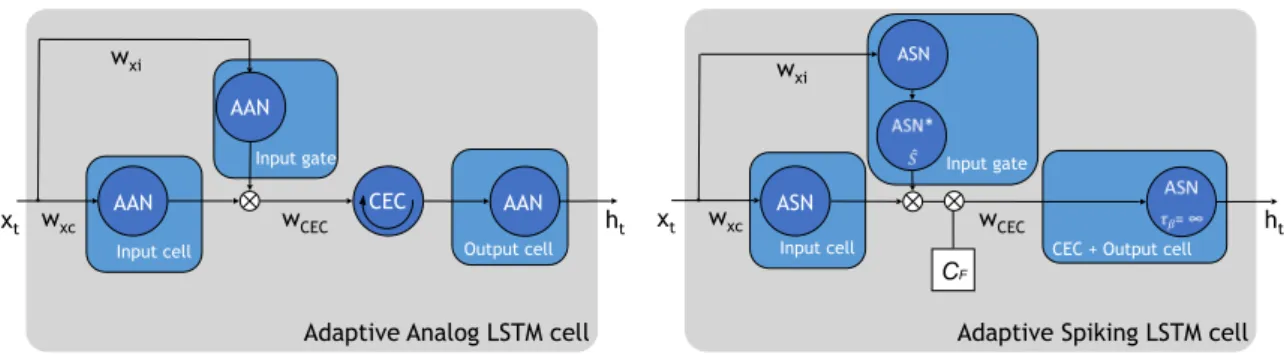
For the part of this project involving the testing of SNNs by means of Machine Learning tasks, an analog LSTM was present in the network during the training phase, and then, in the same way as the rest of the units in the networks, substituted with a spiking counterpart. The unit used here is stripped of many (optional, for the tasks involved in this project) features, such as forget and output gates, or recurrent weights. Moreover, while the original approach (i.e. the one using the analytical transfer function with τη =τγ) used three neurons in order to get the desired transfer function in both the input gate and the input cell of the spiking LSTM (see [56]), here a single neuron is used in both cases, obtaining thus a much more simplified unit. A picture of the old structure is showed in the Appendix.
Overall, the analog LSTM in this project uses a multiplicative input gate, an input cell, a CEC, and an output cell, and the spiking one, instead, is composed only of a
Input cell Output cell Input gate CEC CF AAN AAN AAN Input gate
Input cell CEC + Output cell
ASN
Adaptive Analog LSTM cell Adaptive Spiking LSTM cell
xt ht xt ASN ht wxc wxi w xi wxc wCEC wCEC
Figure 2.4: Overview of the simplified construction of an Adaptive Analog LSTM (left) and an Adaptive Spiking LSTM cell (compare to the architecture showed in the Appendix). This compares to an LSTM with only an input gate.
multiplicative input gate, an input cell, and an output cell. In fact, the spiking CEC was programmed like a normal spiking neuron, but without the decay of the internal state ˆS(t), for which the time constant was theoreticallyτβ =∞, i.e. the exponential was set equal to 1, since it is possible to make the assumption that this decay is very slow for these cells[58]. In Figure 2.4 a depiction of the analog and spiking LSTM is shown: Wxc, Wxi, andWCEC are the weights for the input received by the input cell,
the input gate, and the CEC, respectively, while the ASN* neuron is an intermediate
neuron accumulating the signal coming from the input gate, and its internal state ˆS
is multiplied with the signal going from the input cell to the output cell.
Concerning the update of the CEC, if the ISI can be considered constant the output is increased by ISIh every time step. In the case of a stochastic unit, the mean ISI (i.e. ISI) can be considered constant. Thus, the analog CEC should be updated
by h
ISI =
S
τη (see Equation 2.15, for which the derivation still holds, by assuming
ts:= ISI from the start instead ofts:= ISI). However, in order to simply update the
analog CEC by S, the spiking CEC is instead updated at every time step as follows:
CECstate(t) = CECstate(t−1) +S·CF , (2.26)
where S is the input current entering the CEC. The parameter CF = τη/∆t is a
conversion factor, with ∆t being the time of the spiking simulation, and it needs to
be multiplied to the incoming signal entering the spiking CEC in order to have an accurate conversion from the analog CEC. The analysis of the time component in the two networks represents a crucial point for understanding how to correctly perform the switching from analog to spiking neurons. More in detail, while in the analog environment the input is presented once to the network, in the spiking networks it is required to show the input for several time steps, i.e. milliseconds, in order for the spiking neurons to pass the refractoriness stage (i.e. the phenomenon described in the Introduction for which the neuron needs time in order to adapt to the incoming signal) and to reach a point at which the communicated signal is (to some extent) stable. For this reason, the spiking CEC would store more information than the information
an analog CEC would have accumulated. Hence the ∆t at the denominator in the
2.3
Machine Learning paradigms
In order to test a NN different Machine Learning tasks can be used. In this section the theory of learning is presented, even if it is worth noticing that the focus of this thesis is the optimization of the AAN-ASN conversion.
Overall, it is possible to distinguish between three different types of algorithms, namely supervised learning, unsupervised learning, and reinforcement learning tasks. These terms, to be precise, are not simply algorithms, but they refer both to prob-lems, solution methods, and fields that study those problems and solution methods. Since unsupervised learning algorithms are used for problems such as clustering (their common goal is, in fact, to find hidden structures in sets of unlabeled data), in the present work only the first and the third categories are considered, since they are more related to the type of problems an LSTM network can be deployed for.
Specifically, supervised learning problems refer to situations in which the training consists of comparing the expected output with the output actually produced by the network, and iteratively reducing the residual between these two quantities. The goal of these learning algorithms is to make a system extrapolate its responses so that it will be able to correctly behave in future (unknown) situations. A typical example is handwriting recognition, a widely used supervised learning task for which handwritten figures are shown to the network together with the correct labels for each digit in order for it to find what correlates the input and the expected outputs. This type of tasks are very straightforward and easy to implement, but they require a known set of correct input-output pairs.
On the other hand, during reinforcement learning tasks such a requirement is avoided. In fact, in this case the learning is based on rewarding mechanisms for which an agent tries different possibilities and it is rewarded whenever something is well done, i.e. the same type of process through which biological NNs are supposed to learn[59]. A reinforcement learning system is composed by: an agent, an environment, a policy, a reward signal, a value function, and an (optional) model describing the environment. Reinforcement learning agents have specific goals, can interact with the environment, and can choose actions to take in order to influence it, and they do so while compromising between exploration and exploitation: by exploiting what was already learned, a sensible choice can be already made, but by making more exploration better actions could be made in the future. The policy is a function that maps a state into an action to take, and it is what determines the behavior of the agent. The reward signal is what sets the goal for the agent: each action receives feedback in terms of a reward, which gives to the agent a sense of whether the action that was just taken was good or not, and its final objective is to maximize the total reward receivable. Another indication about which action to choose is given by the value function: it indicates the long-term desirability of an action by giving, in each state, the amount of reward obtainable in the entire run for each possible action that can be taken at that point. Finally, models are used for planning: sometimes it is possible, in fact, to give some a priori knowledge about how the environment will behave.
In the end, it must be mentioned that while deep NNs are widely used for instruc-tive feedback learning (i.e. supervised learning), in order to perform reinforcement learning tasks Deep Learning is not necessary. Other solution methods not
involv-ing deep nets exist, in fact. However, when the sizes of the states and the policy increase, it could be convenient to rely on NNs in order to replace a (quickly in-tractable) table-like policy with more convenient functions providing the greediest actions over time.
Experiments
As explained earlier, the first part of this project involved the mathematical deriva-tion or approximaderiva-tion of new transfer funcderiva-tions, namely an analytical soluderiva-tion and a stochastic one, for the analog neurons. First, the analytical solution with more bio-logically plausible time constants was considered and tested by comparing the update of the analog and spiking CECs. Then, the stochastic solution was derived by means of a fitting procedure, and tested as well. Subsequently, the same stochastic solution was implemented in a LSTM network, with which a Sequence Prediction task and a T-Maze task were trained. For each experiment, the AANs and ASNs described in the previous chapter were used.
3.1
Transfer function
In this section, at first, the experimental setup (i.e. the values for the parameters of the neuronal model) used for testing the analytical transfer function is described. Subsequently, the process leading to the finding of the stochastic solution is presented, followed by, again, the description of the setup used.
3.1.1
Analytical transfer function
The transfer function found in Section 2.2.1 was implemented in Python. The code comprised of a two three-neuron architectures (i.e. one analog and the other spiking), in which the first neuron gave the input, the second was a CEC, and the third neuron acted as a readout. In Figure 3.1 a depiction of the three-neuron system is presented, for both the analog and the spiking case. The simulations were run twice. At first, in
both networks the time constants of the neurons were τη = 30 ms, τγ = 15 ms, while
for the second simulation they were changed toτη = 20 ms,τγ = 10 ms. For both the
simulations, the multiplicative factor and the initial threshold were mf =ϑ0 = 0.1.
Concerning the AANs, the input an readout units were set to have the analytical
transfer function (Equation 2.22) with h = ln
1
mf+1
(i.e. the limit for S → ∞ of
the transfer function, as shown in Equation 2.23), while the state of the CEC was initialized to zero and then updated by means of the expression in Equation 2.26.
AANin CEC AANout I ASNin I ASNreadout CF
Figure 3.1: Three-neuron experiment: architecture implemented in Python and used to test the transfer functions during this project. The top row of neurons represent the analog system, for which an input neuron, a CEC, and an output neuron were deployed; the bottom line of neurons consists of three spiking neurons: an input neuron, a neuron with τβ =∞ (i.e. a CEC), and a readout neuron.
The ASNs, instead, were characterized by having the firing condition in Equation 2.5 and the time constant τφ= 2.5 ms.
Both the analog and the spiking networks were studied for 200 time steps
(mil-liseconds, in the spiking simulation), with an input current I = 1.0 fed into the
system from the 20th till the 180th step. For the purpose of comparing the results, the same simulations were performed for the original transfer function, at first with
τη =τγ = 10 ms and then withτη =τγ = 10 ms.
3.1.2
Stochastic transfer function
In order to find a transfer function for the stochastic AANs able to describe the way an adaptive stochastic neuron works, a code providing the evolution of such a system was written in Matlab. This code depicted an ASN to which a constant input current was fed, and for which the condition of firing was the following:
S−S >ˆ 0, P =Nexp S(t)− ˆ S(t)−ϑ(t)/2 ∆V ! , X < P , (3.1)
where the first equation is needed in order for the neuron to avoid having responses for negative signals (which are not approximated in the case under investigation be-cause not biologically plausible and bebe-cause it would subvert the conversion between analog and digital signals), while the second equation shows the probability of firing (equivalent to the expression in Equation 2.24), and the thir