Short-term stream flow forecasting and downstream gap infilling using machine learning techniques

(1)

downstream gap infilling using machine

learning techniques

by

Melise Steyn

Thesis presented in partial fulfilment of the requirements for

the degree of Master of Science (Applied Mathematics) in the

Faculty of Science at Stellenbosch University

Supervisor: Prof. G.J.F. Smit Co-supervisors: Dr J.M. Wilms

Dr W.H. Brink March 2018

(2)

Declaration

By submitting this thesis electronically, I declare that the entirety of the work contained therein is my own, original work, that I am the sole author thereof (save to the extent explicitly otherwise stated), that reproduction and pub-lication thereof by Stellenbosch University will not infringe any third party rights and that I have not previously in its entirety or in part submitted it for obtaining any qualification.

March 2018

Date: . . . .

(3)

Abstract

Stream flow is an important component in the hydrological cycle and plays a vital role in many hydrological applications. Accurate stream flow forecasts may be used for the study of various hydro-environmental aspects and may assist in reducing the consequences of floods. The utility of time series records for stream flow analyses is often dependent on continuous, uninterrupted ob-servations. However, interruptions are often unavoidable and may negatively impact the sustainable management of water resources. This study proposes the application of machine learning techniques to address these hydrological challenges.

The first part of this study focuses on single station short-term stream flow forecasting for river basins where historical time series data are available. Two machine learning techniques were investigated, namely support vector regres-sion and multilayer perceptrons. Each model was trained on historical stream flow and precipitation data to forecast stream flow with a lead time of up to seven days. The Shoalhaven, Herbert and Adelaide rivers in Australia were considered for experimentation. The predictive performance of each model was determined by the Pearson correlation coefficient, the root mean squared error and the Nash-Sutcliffe efficiency, and the predictive capabilities of the models were compared to that of a physically based stream flow forecasting model currently supplied by the Australian Bureau of Meteorology. Based on the results, it was concluded that the machine learning models have the abil-ity to overcome certain challenges faced by physically based models and the potential to be useful stream flow forecasting tools in river basin modelling. The second part of this study investigates the ability of support vector regres-sion and multilayer perceptron models to infill incomplete stream flow records. The infilling techniques relied upon data from donor stations and rain gauges within close proximity to the station considered for infilling. A case study was conducted on a channel in the Goulburn basin in Australia. The results showed the promising role of machine learning applications for the infilling of gaps in stream flow records and indicated that data from donor stations contribute more to the success of these models compared to precipitation data.

(4)

Uittreksel

Stroomvloei is ’n belangrike komponent in die hidrologiese siklus en speel ’n prominente rol in verskeie hidrologiese toepassings. Akkurate stroomvloei-voorspellings kan vir die bestudering van verskeie hidrologiese omgewingsas-pekte gebruik word en kan help om die nagevolge van vloede te verminder. Die gebruik van tydreeksdata vir stroomvloei-analise is dikwels afhanklik van ononderbroke waarnemings. Onderbrekings is egter dikwels onvermydelik en kan ’n negatiewe impak op die volhoubare bestuur van waterhulpbronne hê. In hierdie studie is die toepassing van masjienleertegnieke met die doel om hierdie hidrologiese uitdagings aan te spreek, bestudeer.

In die eerste gedeelte van hierdie studie is daar op korttermyn stroomvloei-voorspellings by meetstasies wat oor beskikbare historiese tydreeksdata beskik, gefokus. Twee masjienleertegnieke is ondersoek, naamlik steunvektor-regressie en multi-laag perseptron modelle. Elke model is op historiese stroomvloei- en reënvaldata afgerig om stroomvloei tot en met sewe dae vooruit te voorspel. Eksperimente is op die Shoalhaven, Herbert en Adelaide riviere in Austra-lië uitgevoer. Die voorspellingsvermoëns van elke model is deur die Pearson-korrelasiekoëffisiënt, die wortel-gemiddelde-kwadraat fout en die Nash-Sutcliffe-doeltreffendheid bepaal, en is met dié van ’n fisiese stroomvloeivoorspellings-model wat tans deur die Australiese Buro vir Meteorologie verskaf word, ver-gelyk. Op grond van die resultate is daar tot die gevolgtrekking gekom dat die masjienleermodelle oor die vermoëns beskik om sekere uitdagings waar-mee fisiese modelle gekonfronteer word, te oorkom, en dat hulle ’n waardevolle bydrae tot die modellering van riverkomme kan lewer.

In die tweede gedeelte van hierdie studie is steunvektor-regressie en multi-laag perseptron modelle se vermoëns om onvolledige stroomvloeistate te vul, ondersoek. Die invultegnieke was afhanklik van data vanaf ander nabygeleë meetstasies en reënmeters. ’n Gevallestudie is op ’n kanaal in die Goulburn opvangsgebied in Australië uitgevoer. Die resultate het die belowende rol van masjienleertoepassings op die invul van gapings in stroomvloeistate getoon en aangedui dat data van meetstasies ’n groter bydrae tot die sukses van hierdie modelle lewer in vergelyking met reënvaldata.

(5)

Acknowledgements

All glory be to God Almighty, my Heavenly Father, Saviour and Ultimate Teacher for making the completion of this study a reality. What a privilege to serve and worship a God who answers my prayers, renews my strength, gives me insight and loves me unconditionally. I will forever be thankful for all the opportunities that He has blessed me with. “God arms me with strength, and he makes my way perfect. He makes me as surefooted as a deer, enabling me to stand on mountain heights. You have given me your shield of victory. Your right hand supports me; your help has made me great.” Psalm 18:32-33,35 I would also like to express my sincere appreciation to the following individuals and institutions who contributed to the completion of this research:

The Modelling and Digital Science (MDS) unit of the Council for Scientific and Industrial Research (CSIR), for funding my studies since 2012. They made my dream of studying at Stellenbosch University a reality, and also gave me the financial support to present my work at a conference in Spain earlier this year. A special thank you to my managers, Dr Onno Ubbink and Dr Kobie Smit, for always going the extra mile for the MDS group, and to my colleagues at the CSIR for their constant support and encouragement the past two years. My supervisors, Prof. Francois Smit and Dr Willie Brink at Stellenbosch Uni-versity, and Dr Josefine Wilms at the CSIR, for providing invaluable guidance and assistance. Their critical appraisals, suggestions and keen eye for detail have contributed greatly to the completion of this study.

My beloved parents, Francois and Sharon du Toit, and brother, Francois, for their endless love, support, prayers and encouragement. Words cannot describe how thankful I am for the tremendous sacrifices that my parents have made to ensure an excellent education and endless opportunities. I would also like to express my gratitude to my parents-in-law and friends who have never ceased to pray for me.

My biggest support, my cheerleader, my best friend, my greatest love, my husband: Wim Steyn. His infectious excitement about life, his purpose-driven lifestyle and his unfailing love, encouragement and support have made these past two years not only bearable, but also memorable. Thank you for being the best husband any wife could possibly have.

(6)

Nomenclature

Variables

ai Output of node i in particular MLP layer

b Bias in MLP formulation c Variable in SVR formulation

C Penalty parameter in SVR formulation d Forecasting lead time (days)

D Stream flow at downstream station (ML/day) Margin of error in SVR formulation

fi Forecasted output variable

f Mean forecasted output variable

h Number of hidden nodes in an MLP model K Number of folds considered for cross-validation l Lag time (days)

m Number of output variables in the test set n Number of training samples

N Number of input nodes in an MLP model

NSE Nash-Sutcliffe efficiency

p Number of preceding precipitation values in the input vector

of the machine learning model

P Precipitation (mm)

q Number of preceding stream flow values in the input vector

of the machine learning model v

(7)

NOMENCLATURE vi

Q Stream flow (ML/day)

r Pearson’s correlation coefficient RMSE Root mean squared error

s Step size in MLP optimisation algorithm t Current day

u Number of preceding stream flow values from upstream station

in the input vector of a machine learning model

U Stream flow at upstream station wij Weight connecting layer i with layer j

xi Input variable

x Mean input variable X Original input space yi, y True output variable

y Mean true output variable

z Weighted sum of a specific MLP node’s input α, α∗, η, η∗ Lagrange multipliers

γ, r, v Kernel-specific hyperparameters in SVR λ Dual variable

µ Mean value of a dataset

ξ, ξ∗ Slack variables in SVR formulation σ Standard deviation of a dataset

Φ(X) Feature space

Vectors

d Direction of descent f Forecasted output vector Q Stream flow vector (ML/day)

(8)

NOMENCLATURE vii

w Weight vector x Input vector

y True output vector

Matrices

H Hessian matrix

Functions

E Error function

floss -insensitive loss function

f(x) Target function

g Activation function k Kernel function

LD Dual Lagrangian function

LP Primal Lagrangian function

Abbreviations

BOM Bureau of Meteorology CDO Climate Data Online

HRS Hydrologic Reference stations IDW Inverse distance weighting

L-BFGS Limited-memory Broyden-Fletcher-Goldfarb-Shanno MLP Multilayer perceptron

RBF Radial basis function SVM Support vector machine SVR Support vector regression Subscripts

(9)

Chapter 1

Introduction

1.1

Motivation

Stream flow is an important component in the hydrological cycle and plays a vital role in many hydraulic and hydrological applications. Research on model-generated stream flow is used by river engineers and scientists for the study of various hydro-environmental aspects, such as the increasing international concern of riverine pollution and the growing flood stages of rivers (Falconer

et al., 2005). Consequences of natural disasters, such as floods, can be lessened

or even prevented through accurate stream flow forecasts (Raghavendra and Deka, 2014).

Modern river basin management, based on the prediction of stream flow and the analysis of different environmental scenarios, is reliant on the adequacy of the particular hydrological model used (Falconer et al., 2005; Solomatine and

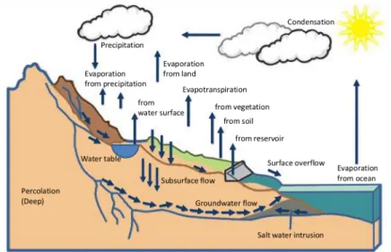
Ostfeld, 2008). A popular conventional model for stream flow forecasting is a physically based rainfall-runoff model. This model is used to transform rain-fall estimations to runoff, which in turn may be used to determine stream flow by modelling the hydrologic processes within a catchment. As illustrated in Figure 1.1, these processes typically include interception, infiltration, evapora-tion, snowmelt, retention and detention storages, soil water movement, perco-lation to ground water, overland flow, open channel flow and subsurface flow (Knappet al., 1991). According to Perrinet al.(2003), it can be challenging to

choose an appropriate model structure and complexity for accurate simulation of hydrological behaviour at catchment scale. If the model is too simple, it might prevent sufficient flexibility for an adequate representation of hydrolog-ical events within the catchment, whereas a model that is too complex may result in model robustness problems (Perrin et al., 2003). These challenges

might limit the modelling accuracy of a physically based model.

During the past decade, major progress has been made in the study of data-driven models to simulate hydrological processes within a catchment

(12)

CHAPTER 1. INTRODUCTION 2

Figure 1.1: An illustration of the hydrological processes that have to be taken into account when modelling stream flow with a physically based rainfall-runoff model, redrawn from Encyclopaedia Britannica (2017).

matine and Ostfeld, 2008). Data-driven models are based on observed data that characterise the system under study. While physically based models in-volve equations derived from physical processes within the specific system, data-driven models include equations obtained from analysing time series data (Solomatine and Ostfeld, 2008). Various processes within a river basin are characterised by measurable state variables, such as stream flow, precipita-tion, temperature and humidity. A river basin for which time series records are available may therefore be a good candidate for the implementation of data-driven models.

The utility of time series records for stream flow analyses is often dependent on continuous, uninterrupted observations. The production and management of hydrometric data over a long period of time is, however, a challenging task. Technical or maintenance problems of a gauging station may affect its ability to generate flow measurements and may result in an incomplete dataset. Factors responsible for discontinuities in available records include the malfunctioning of equipment, flood damages, infrequent calibration of sensors and upgrades to existing equipment for more sophisticated measuring techniques. Gaps in a time series record indicate a loss of information and, according to Tencaliec

et al. (2015), may lead to inaccurate and unreliable hydrological analyses.

Incomplete datasets increase the complexity and uncertainty of hydrological modelling, and even very small gaps may prevent the accurate analysis of fun-damental statistical information such as mean daily runoff volumes, or the reliable interpretation of flow variability (Campozano et al., 2014).

Conse-quently, to avoid the effect of incomplete records on hydrological studies, and to make these studies more reliable, it is crucial to implement techniques that can perform estimations from incomplete records. According to Tencaliecet al.

(13)

CHAPTER 1. INTRODUCTION 3 (2015), this is termed the reconstruction, imputation or infilling of a dataset.

1.2

Objectives and domain of this study

This study proposes the application of modern data-driven modelling tech-niques, also known as machine learning, to address two hydrological problems discussed in Section 1.1: stream flow forecasting and gap infilling. Support vector regression and multilayer perceptron models will be considered, due to their popularity and applicability to various problems related to river basin management (Borji et al., 2016).

The first objective of this study is to investigate single station short-term stream flow forecasting at a specific location in a river channel, by considering stream flow and precipitation time series records at that particular forecasting location. Three Australian river stations with sufficient time series records will be investigated. Support vector regression and multilayer perceptron models will be trained on the historical data of the stations to forecast stream flow with a lead time of up to seven days. The predictive capabilities of the machine learning models will be compared to that of a rainfall-runoff model provided by the Bureau of Meteorology (BOM), Australia’s national weather and cli-mate agency. They provide a forecasting service that supplies stream flow predictions at more than 100 locations across Australia. These forecasts are

determined by a system which uses a rainfall-runoff model known as GR4J as its main component (Perrin et al., 2003). This daily lumped, conceptual, four

parameter, soil moisture accounting rainfall-runoff model determines the total amount of rainfall in a specific catchment, the fraction of rainfall that ends up as runoff, and the accumulation of that runoff in downstream rivers (Perrin

et al., 2003). Stream flow forecasts are given for a lead time of up to seven

days (as shown in Figure 1.2), and are used for several water management purposes.

Secondly, we will investigate the ability of support vector regression and multi-layer perceptron models to infill incomplete stream flow records. A particular case will be addressed where two different gauging stations are located along a river channel: one with an uninterrupted stream flow record, and the other one with gaps. The purpose of this part of the study is to infill the missing stream flow values of the one gauging station by considering the stream flow record of the other station, as well as data from any rain gauges within close proximity to the station considered for infilling.

The contribution of this study resides in the analysis of results. This includes the extent to which different environmental factors affect both machine learn-ing and physically based model performances, which provides environmental researchers with insight into which climate variables may have a significant

(14)

CHAPTER 1. INTRODUCTION 4

Figure 1.2: The forecasting service web portal provided by the Australian Bureau of Meteo-rology. Stream flow and rainfall forecasts with a lead time of up to seven days are provided to help river users in making decisions related to river and reservoir operations and water management (Bureau of Meteorology, 2017).

effect on stream flow. Furthermore, emphasis will be placed on good practices for machine learning system design in the field of hydrology.

1.3

Thesis layout

This thesis is organized into six chapters. Chapter 1introduces current issues

in the field of hydrology regarding stream flow modelling techniques and time series analyses. The rationale for the study, the objectives, scope and general research methodology are outlined. Furthermore, the publications from this study are listed.

Chapter 2 explains how hydrographs can be used to illustrate the effects of

rainfall events on stream flow, and discusses the climatic and physiographic factors affecting their shape. Understanding the response of a given catch-ment’s stream flow to rainfall input is helpful when choosing input features for the machine learning models, and may also give insight to the performance of

(15)

CHAPTER 1. INTRODUCTION 5 the models.

Chapter3provides a review of machine learning fundamentals, including

train-ing, validation, testtrain-ing, data preparation and performance evaluation. A de-tailed description of the two modelling techniques considered for this study, namely support vector regression and multilayer perceptrons, is given and their advantages and drawbacks are outlined.

Chapters4and5describe techniques used in the development of support vector

regression and multilayer perceptron models for short-term stream flow fore-casting and gap infilling. Descriptions of the study areas and available datasets are given. Data analysis, feature selection, preprocessing and model perfor-mance evaluation techniques are discussed in detail. Furthermore, methods for choosing support vector regression hyperparameters and multilayer per-ceptron architectures are given. These chapters also present the results of the forecasting and gap infilling models, and their performances are discussed. Chapter 6presents concluding remarks based on our findings from Chapters4

and 5. Recommendations for future research are also given.

1.4

Publications from this study

National conference paper

• Du Toit, M., Wilms, J.M., Smit, G.J.F. and Brink, W. (2016). The application of support vector regression (SVR) for stream flow prediction on the Amazon basin. 32nd Annual Conference of the South African Society for Atmospheric Science, Cape Town, 31 October - 1 November

2016. ISBN 978-0-620-72974-1, pp. 25–28. International conference paper

• Steyn, M., Wilms, J., Brink, W. and Smit, F. (2017). Short-term stream flow forecasting at Australian river sites using data-driven regression techniques. 4th International Work-conference on Time Series Analysis,

Granada, Spain, 18-20 September 2017. ISBN 978-84-17293-01-7, pp. 865–876.

(16)

Chapter 2

Stream flow and hydrographs

Stream flow or discharge is the volume of water that flows past a specific location in the river bed per unit time, and is usually measured at gauging stations situated along the river. Stream flow is a dynamic process that con-stantly changes due to various environmental factors. A hydrograph shows changes in stream flow at a specific location as a function of time and can be plotted in conjunction with a hyetograph (a graphical representation of rain-fall intensity over time) to illustrate effects of preceding rainrain-fall events, also referred to as storms, on stream flow.

Hydrologists assess the behaviour and performance of a hydrological model by estimating how well the observations made within the catchment are pre-dicted. When considering stream flow modelling, a fundamental approach to evaluate model performance is through visual inspection of observed and fore-casted hydrographs (Krauseet al., 2005). Hydrologists can assess whether the

forecasted model over- or underpredicts actual stream flow, whether increas-ing and decreasincreas-ing flow are accurately replicated, and whether the timincreas-ing of the dynamic behaviour of the model is correct (Krause et al., 2005). Since

this approach will also be used to assess the results of our data-driven models, the main aspects of a hydrograph and the factors affecting its shape will be discussed.

2.1

Hydrograph shape

A hydrograph consists of two main components: base flow and overland flow. Base flow is the portion of stream flow supplied by groundwater. Overland flow is produced as a result of a rainstorm, and manifests in the form of surface runoff or through flow. Surface runoff is the water that flows directly over the land surface until it reaches the channel, whereas through flow is the lateral unsaturated flow of water in the soil zone which returns to the surface before entering the stream or becoming groundwater. The duration of

(17)

CHAPTER 2. STREAM FLOW AND HYDROGRAPHS 7

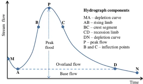
Figure 2.1: The main components of a typical hydrograph at a particular point in the river channel during a single storm, redrawn from Subramanya (2009).

overland flow is referred to as the hydrograph time base, and the total runoff obtained from overland flow is represented by the remaining area above the base flow on a hydrograph. The boundary between overland flow and base flow is dependent on the catchment structure and composition and may be challenging to determine.

The hydrograph shape represents the time distribution of runoff and follows a typical pattern when a single storm occurs over the catchment area. The main components of a hydrograph are the rising limb, the crest segment and the recession limb, as indicated in Figure 2.1 (Subramanya, 2009).

2.1.1

Rising limb

The rising limb of a hydrograph, represented by AB in Figure 2.1, describes a rise in stream flow as a result of channel and catchment surface storage slowly building up (Subramanya, 2009). During the initial stages of a storm, rainfall is first lost to processes such as interception and infiltration, causing a time delay before the rainfall excess reaches the stream and leads to a slow rise in stream flow (Wisler and Brater, 1959). The portion of rainfall contributing to stream flow is termed effective rainfall, whereas the remainder is evaporated, retained in the soil or detained on the land surface. A prolonged storm leads to an increase in effective rainfall, since infiltration losses decrease and more flow from distant parts of the catchment reaches the basin outlet (Subramanya, 2009). The slope of the hydrograph’s rising limb therefore increases rapidly with time.

(18)

CHAPTER 2. STREAM FLOW AND HYDROGRAPHS 8

2.1.2

Crest segment

An important feature of a hydrograph’s crest segment, represented by BC in Figure 2.1, is the peak flow, defined as the maximum flow at the basin outlet (Subramanya, 2009). For larger catchments, the peak flow may occur even after the storm has ended. The time difference between the effective rainfall’s centre of mass to the peak flow of the hydrograph is referred to as the basin lag time, and is primarily determined by basin and storm characteristics (Sub-ramanya, 2009). It is important in flood-flow studies to be able to determine the magnitude of a channel’s peak flow as well as the time of its occurrence.

2.1.3

Recession limb

The recession limb, represented by CD in Figure 2.1, describes the depletion of storage, i.e. the removal of water from storage that accumulated in the basin during the beginning stages of the storm (Linsey et al., 1949; Subramanya,

2009). Three main forms of water storage exist: surface storage (consisting of channel storage and surface detention), interflow storage, and groundwater or baseflow storage. The inflection point at the end of the crest segment, represented by C in Figure 2.1, corresponds to the basin’s state of maximum storage (Subramanya, 2009). Storage depletion only occurs after the storm has ended. The shape of the recession limb is therefore dependent only on basin characteristics and not on storm characteristics (Linsey et al., 1949).

The relation between base flow and time is expressed by the lower part of a hydrograph’s recession limb and is also known as the depletion curve (Wilson, 1974). The depletion curve is shown by DN in Figure 2.1, and indicates when the stream flow is entirely a result of groundwater seepage.

2.2

Ephemeral, intermittent and perennial

rivers

A river may be classified as ephemeral, intermittent or perennial, based on the position of the catchment’s water table (Roy et al., 2009). Ephemeral streams

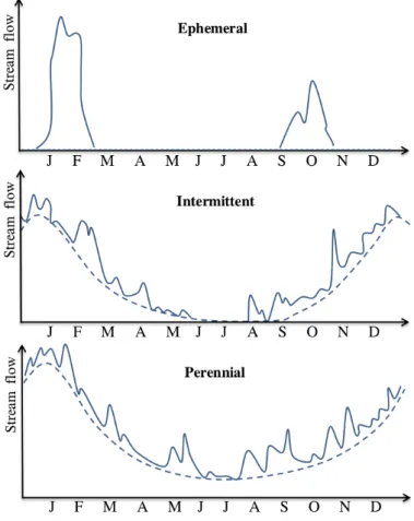
consist of channels that are always above the water table. The existence of the stream is therefore completely dependent on effective rainfall. Streams that are seasonally dependent are defined as intermittent. The water table of an intermittent stream lies above the river bed during wet seasons and drops to a depth below the bed in dry seasons. During dry seasons, these rivers are dependent on effective rainfall for flow, whereas groundwater is contributed to the channels during the wet seasons. Perennial streams are river channels con-sisting of continuous flow throughout the year. The water tables of perennial streams are permanently above certain parts of the channel bed, constantly providing water to the stream. Characteristic hydrographs for the three types

(19)

CHAPTER 2. STREAM FLOW AND HYDROGRAPHS 9 of rivers are shown in Figure 2.2. Due to storm and basin irregularities as well as their complicated interactions, many of these hydrograph shapes may contain kinks and multiple peaks that differ from the simple single-peaked hydrograph in Figure 2.1.

2.3

Factors affecting a hydrograph

The shape of a hydrograph is dependent on many climatic and physiographic factors, also known as drainage basin controls. Table 2.1 lists the most im-portant drainage basin controls, according to Subramanya (2009). Climatic factors mainly determine the rising limb, whereas physiographic factors affect the recession curve. A more detailed discussion on the main drainage basin controls and their effects on the hydrograph shape follows, assuming that the basin outlet is considered as the location where the stream flow is measured.

Figure 2.2: Typical hydrographs of the three types of rivers over a one year period. The dashed curves indicate the base flow of each type of river, whereas the solid curves show the hydrographs during storms.

(20)

CHAPTER 2. STREAM FLOW AND HYDROGRAPHS 10

Table 2.1: Climatic and physiographic factors affecting the hydrograph.

Climatic factors Physiographic factors 1. Storm characteristics 1. Basin characteristics

(a) intensity (a) size (b) duration (b) shape (c) distribution (c) slope

(d) direction (d) drainage density

(e) type (e) elevation

2. Evapotranspiration 2. Infiltration characteristics (a) land-use and vegetation (b) soil type

(c) storage (lakes and swamps) 3. Channel characteristics

(a) cross-section (b) roughness (c) storage capacity

2.3.1

Climatic factors

The hydrograph shape and the amount of runoff that reaches the outlet are influenced predominantly by four climatic factors: the intensity, duration and distribution of a storm over the catchment, and the direction in which the storm moves.

Storm intensity

Storm intensity is defined as the amount of rainfall (in depth) per unit time and has an influence on the peak flow and the total volume of surface runoff for a given soil infiltration rate. A rainfall intensity that exceeds the soil’s infiltration rate causes more overland flow and results in a steeper rising limb (Wisler and Brater, 1959).

Storm duration

Storm duration determines the peak flow and the duration of surface runoff, assuming a uniform storm intensity over the total catchment area (Wisler and Brater, 1959). An isochrone map consists of lines connecting points from which the runoff will take the same amount of time to reach the basin outlet, and may be useful in describing the effect of storm duration on the hydrograph of the catchment. Figure 2.3 illustrates a catchment where the point of measurement is at the outlet. When a storm occurs, the slope of the hydrograph’s rising limb will start to increase. After a time ∆t, the water from isochrone I would have

reached the outlet and the whole area represented byAIwould be contributing to the rising limb. After a time period of 2∆t, the water from isochrone II

(21)

CHAPTER 2. STREAM FLOW AND HYDROGRAPHS 11 would have reached the outlet and the whole area represented by AI and AII would contribute to the rising limb. If the rainfall continues until the entire catchment area contributes to the rising limb, the river is said to have reached its time of concentration (Linsey et al., 1949). The hydrograph would reach a

peak flow equal toreA, wherererepresents storm intensity andAthe total area of the basin. The point of concentration may be reached in smaller catchments, and is therefore commonly used as the criterion for infrastructure development (such as bridges and culverts) and stormwater management (Saghafian and Julien, 1995).

Figure 2.3: An isochrone map, consisting of lines (isochrones) that connect points from which the runoff will take the same amount of time to reach the basin outlet.

Storm distribution

The possible impact of storm distribution on the hydrograph shape can be ex-plained by considering the isochrone map in Figure 2.3. If the storm is centred in an area near the basin outlet (such as AI), the resulting hydrograph will show higher peak runoff compared to a storm centred in an area further away from the outlet (such as AIV) (Linsey et al., 1949; Wisler and Brater, 1959). According to Wisler and Brater (1959), rain that is uniformly distributed over a catchment produces the minimum peak runoff for a given total volume of rainfall and catchment characteristics.

Direction of storm movement

The direction in which a storm travels over a catchment with respect to the direction of river flow affects the resulting peak flow and the duration of surface runoff (Wisler and Brater, 1959). Elongated catchment areas are especially affected by the direction of a storm. If the point of flow measurement is considered to be at the outlet, a storm moving in an upstream direction would result in lower peak flow and a longer time base. Conversely, a storm moving

(22)

CHAPTER 2. STREAM FLOW AND HYDROGRAPHS 12 towards the downstream end leads to more rapid flow concentration at the outlet, resulting in higher peak flow and a shorter time base.

2.3.2

Topographic and geologic factors

The physical characteristics of a catchment are described by topographic and geologic factors and affect the shape of a hydrograph during a storm. These factors include the catchment shape, size, slope, drainage and land-use. Catchment size

Smaller catchments show a different runoff behaviour compared to larger catch-ments, due to a difference in the relative importance of the existing runoff phases. In a smaller catchment, the overland flow phase has the greatest effect on the peak flow of the hydrograph, whereas the channel flow phase is more influential in a larger catchment (Subramanya, 2009). The time base of hy-drographs for a smaller catchment will be shorter compared to that of a larger catchment, since water at the most remote point from the outlet has a shorter distance to travel.

Catchment shape

The shape of a catchment affects the time it takes water from the remote parts of the basin to reach the outlet point and therefore influences the result-ing peak flow (Wisler and Brater, 1959). A catchment with a semi-circular or fan shape leads to a narrow and high-peaked hydrograph, whereas an elongated catchment shape gives a broad and narrow-peaked hydrograph (Subramanya, 2009). Figure 2.4 shows the effect of three different catchment shapes on a hydrograph, assuming identical rainfall and infiltration characteristics. Catch-ment A has a narrow end towards the upper basin area and a broader end towards the basin outlet, and will therefore result in a peak with a shorter drainage lag time. Catchment B has a broader end towards the upper basin area and a narrow end towards the basin outlet, and will therefore lead to a peak with a longer drainage lag time. Catchment C shows the hydrograph shape that results from a catchment with a composite shape.

Catchment and main stream slope

The slope of a catchment’s main stream channel greatly affects the stream velocity and rate of storage depletion, and therefore alters the shape of a hy-drograph’s recession limb (Subramanya, 2009). A larger slope generates a greater velocity and causes more rapid storage depletion, resulting in a steeper recession limb and a smaller runoff time base. The catchment slope is essential in smaller catchments, since overland flow is more predominant than in larger

(23)

CHAPTER 2. STREAM FLOW AND HYDROGRAPHS 13

Figure 2.4: Effect of different catchment sizes on a hydrograph shape (Subramanya, 2009).

catchments (Subramanya, 2009). A catchment with a greater slope will there-fore lead to larger peak flow values, compared to a catchment with a smaller slope.

Drainage

An important catchment characteristic is the arrangement of the natural stream channels in the area. Basins that are well drained allow a quicker disposal of runoff down the river, and causes a larger peak flow and a shorter drainage lag time compared to poorly drained basins (Wisler and Brater, 1959). Figure 2.5 illustrates the effect of a basin’s drainage on the hydrograph shape, given that all other catchment and climatic characteristics remain identical.

Figure 2.5: Effect of a catchment’s drainage on the hydrograph shape (Subramanya, 2009).

Catchment land-use

The way in which the land within a catchment is utilised greatly influences the resulting peak flow (Wisler and Brater, 1959; Subramanya, 2009). Veg-etation and forests intercept rainfall, increase the soil’s storage capacity and delay overland flow. Therefore, less runoff reaches the river channel and over a longer period of time, resulting in a hydrograph with lower peak flow and a

(24)

CHAPTER 2. STREAM FLOW AND HYDROGRAPHS 14 longer drainage time lag and base. An urbanised area, consisting of imperme-able surfaces such as roads and bridges, hinders the rainfall from infiltrating the surface. More rainfall reaches the channel as overland flow, resulting in increased peak flow and shorter drainage lag time.

(25)

Chapter 3

Data-driven modelling

Times series modelling is a dynamic research field that has evoked the attention of many research communities over the past few decades and has progressed significantly since 1970 (Adhikari and Agrawal, 2013; Box and Jenk-ins, 1970). Conventional linear models such as autoregressive moving average, autoregressive integrated moving average, linear regression and multiple lin-ear regression models were developed and used for stream flow forecasting (Yaseen et al., 2015). A drawback of these models, however, is their inability

to adapt to nonlinear relationships in the data. Due to this limitation, more so-phisticated data-driven modelling techniques were developed (Solomatine and Ostfeld, 2008).

Data-driven modelling is based only on data and is used to predict, but not necessarily explain, processes within a system. Developments in the area of machine learning have expanded the capabilities of data-driven modelling sub-stantially (Solomatine et al., 2008). Machine learning models analyse time

series data to obtain functions that capture trends within the data. Numerous machine learning techniques have been applied to various hydrological pro-cesses, such as sediment transport, groundwater, water quality, precipitation, evapotranspiration, evaporation, floods, droughts and water levels (Yaseen

et al., 2015).

3.1

Fundamentals of machine learning

A central purpose of machine learning is to construct a model from historical data of the system under study, for the purpose of making predictions for that specific system from previously unseen data. The process of using available historical data to find a mapping between input and output data of a system is known as learning. As illustrated in Figure 3.1, the learning procedure aims to minimise the difference between actual observed output and predicted output (Solomatine and Ostfeld, 2008). When using machine learning to model a

(26)

CHAPTER 3. DATA-DRIVEN MODELLING 16

Figure 3.1: Supervised learning process, redrawn from Solomatine and Ostfeld (2008).

system, a sufficient amount of data characterising that specific system needs to be available.

Learning techniques can be distinguished based on the information available in the data. Specifically, if each available sample is a pair containing an input and output value (also known as a label), supervised learning can be considered. A supervised learning model aims to find the best target function f for the

output y given its corresponding input x, as illustrated in Figure 3.1. The given dataset is analysed, dependencies between the inputs and outputs are found, and a mapping y =f(x) is constructed. After f is determined, it can

be used for mapping new, previously unseen inputs. The process of learning a target function f is also known as training. Another type of learning can

be used on datasets consisting of inputs and no corresponding outputs, and is called unsupervised learning. These methods analyse the dataset and cluster the data into different classes based on patterns or similarities found in the data.

A supervised learning model that predicts continuous variables is referred to as a regression model. If a model is used to categorise or predict discrete class labels, it is known as a classification model. Since hydrologically based problems are usually required to predict continuous variables such as stream flow or water levels, a regression model is considered.

3.1.1

Training, validation and testing

It is important to understand the methodology for using data when developing a machine learning model. A dataset is typically divided into three subsets, known as the training, validation and test sets. The data samples in the training set are used in learning a target function, as previously mentioned. During learning, the model complexity may increase to produce decreasing errors on the training data (Bray and Han, 2004; Solomatine and Ostfeld, 2008). However, when considering only the training set in the construction of a model, the problem of overfitting may occur. Overfitting is caused when the model learns the detail and noise in the training set to an extent that its performance on new unseen data (also referred to as the test set) is impacted

(27)

CHAPTER 3. DATA-DRIVEN MODELLING 17 negatively. The model complexity is increased to fit the data samples in the given training set well, but large prediction errors are caused on unseen data. On the other hand, underfitting describes a model with low model complexity that can neither properly model the training data nor generalise to new unseen data.

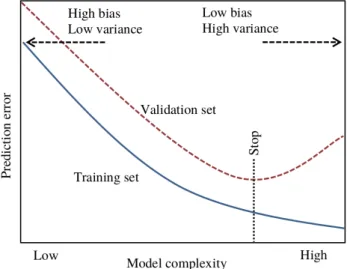
We therefore aim to train a model that generalises well to unseen data, and do so by introducing the validation set. During training, the model is tested by fitting it to the validation set. At first, the error on both the training and validation sets will decrease as the model complexity increases. However, at a certain point the validation error may start to increase as an effect of overfit-ting. As illustrated in Figure 3.2, the training process should be terminated at this point.

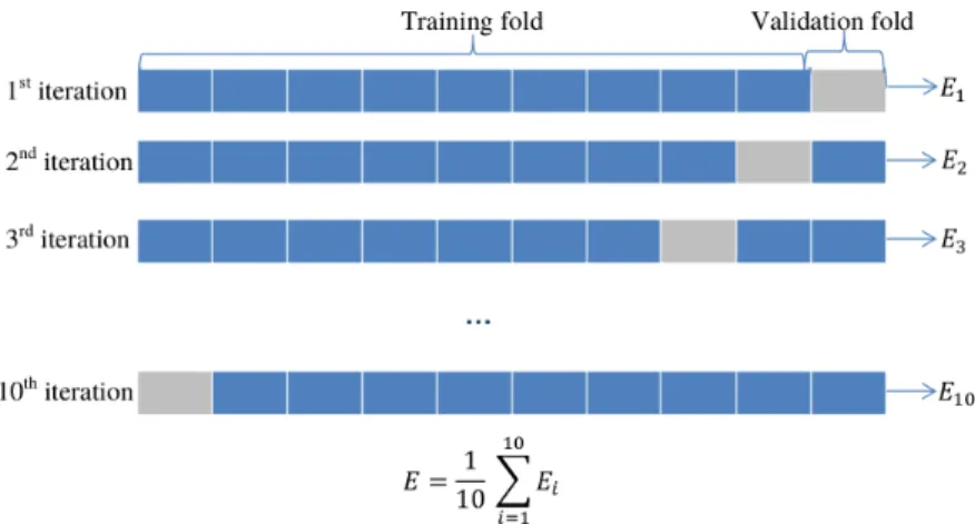
A more sophisticated generalisation approach is known as K-fold cross

vali-dation, where the training set is split into K folds of equal size. Each fold is

considered as a validation set once while the remaining K−1 folds are used

as the training set, as illustrated in Figure 3.3. The best trained model or a weighted combination of all trained models can then be used as the final model (Hastie et al., 2009; Solomatine and Ostfeld, 2008). K-fold cross validation

also maximises utilisation of the data, especially when only a small set of data is available (Maier and Dandy, 2000).

A further way of improving a model’s ability to generalise to unseen data is to ensure that the training and validation sets are representative of the same population (Solomatine and Ostfeld, 2008; Maier and Dandy, 2000). For

Figure 3.2: Generalisation of a machine learning model, redrawn from Bray and Han (2004). A model with low complexity may cause underfitting and result in large training and vali-dation errors, whereas a model with high complexity may lead to overfitting by obtaining small training errors but large validation errors. A generalised model may be obtained by stopping the training process when a minimum validation error is obtained.

(28)

CHAPTER 3. DATA-DRIVEN MODELLING 18

Figure 3.3: An illustration of10-fold cross validation. The full training dataset is split into

10folds of equal size. Each fold is considered as a validation set once, while the remaining 9 folds are combined to form a training set. Ultimately, the model with the lowest validation error on all 10 trials, or a weighted combination of all 10 models can be used for forecasting purposes. The error function E is computed as the sum of the squared difference between the true outputs and the network outputs.

instance, if a model is built to predict weather conditions of a specific region, the training set should contain data samples representing all four seasons of the year.

3.1.2

The bias-variance trade-off

The prediction error made by a machine learning model can be categorised as irreducible, bias, or variance. Irreducible errors are introduced in the model formulation of the problem and cannot be lessened by modifying the target function. Such errors may occur due to external factors that affect the way inputs are mapped to the outputs, but are not taken into consideration when constructing the model. For instance, consider modelling the water level of a dam, using rainfall measurements for that specific region. Due to the strong relationship between the input and output data, the resulting target function might be able to map the training data well. However, since other factors that influence the amount of water accumulating within the dam (such as temperature and evaporation) are not considered in the formulation of the model, an irreducible error might be present.

Bias indicates the difference between the expected prediction of a training model and the true value that it is trying to predict. Consider determining the target function for a set of data samples describing a specific process. By resampling the dataset, the model building process can be repeated many times to obtain an average model or target function. Bias refers to the difference between the predicted values of the average model and the true values. The

(29)

CHAPTER 3. DATA-DRIVEN MODELLING 19 greater the difference, the higher the bias. A function with high bias may miss relevant relations between input and output data, and may therefore lead to errors when making predictions.

Variance refers to the amount of change in the predictions of the target function when considering different data samples. A model with high variance varies drastically from one dataset to another and may lead to unreliable predictions. High-complexity models may have high variance, since a small change in the dataset can cause a significant change in the shape of the target function. An objective in constructing a supervised machine learning model is to ob-tain both low bias and low variance, since such a target function is likely to have good prediction performance. However, the difficulty in satisfying these requirements lies in the fact that a decrease in bias can lead to an increase in variance. Similarly, a decrease in variance can lead to an increase in bias. This is known as the bias-variance trade-off, and is also indicated in Figure 3.2.

3.1.3

Preparation of data

The preprocessing of data and the choice of variables that describe a modelled system can have a significant effect on model performance (Maier and Dandy, 2000; Solomatine and Ostfeld, 2008). One method of choosing variables is to rely upon the knowledge of a domain expert, who has an understanding of the hydrologic system that is being modelled (Bowdenet al., 2005). More

for-mal methods have been developed to justify the choice of input features. For instance, linear cross-correlation is a popular analytical approach that deter-mines the similarity between potential input features and the modelled process. If the similarity is strong, the considered feature may be a promising candi-date for training the model. Imrie et al.(2000) built a stream flow forecasting

model and considered cross-correlation analyses to determine appropriate lags of time series from upstream gauges as inputs. Various other examples of how cross-correlation have been used in hydrological studies are given by Bowden

et al. (2005). However, a notable disadvantage concerning cross-correlation is

its inability to capture nonlinear dependencies between inputs and outputs. A commonly used heuristic approach for input feature selection is the stepwise technique. It is based on trial and error and considers different subsets of in-put. The two main stepwise approaches are known as forward and backward selection. Forward selection starts by finding the single best input feature for the final model. A set of selected input features are then considered, from which the feature that improves the model’s prediction capabilities most is added to the final model. This process is repeated for all selected subsets of input features. Backward selection first considers all input features in a set. In each subsequent step, the input feature that reduces the performance the most is eliminated. Tokar and Johnson (1999) used the forward selection

(30)

ap-CHAPTER 3. DATA-DRIVEN MODELLING 20 proach to find the input features for forecasting daily runoff in a watershed in the USA. A drawback of these heuristic approaches is that they can be com-putationally expensive. Furthermore, since they are based on trial and error, the globally optimal subset might not be found (Bowden et al., 2005). Many

other feature selection techniques have been developed and successfully imple-mented, including the stepwise partial mutual information algorithm (Bowden

et al., 2005) and the singular spectral analysis technique (Wang et al., 2015).

Deep learning is a subfield of machine learning methods that is useful in cir-cumventing the challenges of feature extraction. Deep learning models are able to learn how to extract an optimal feature vector for the given dataset using data compression algorithms known as autoencoding (Nezhad et al., 2016).

Autoencoders are especially useful when very large datasets are available for training.

For many machine learning models, data transformation is an important aspect of preprocessing. Two basic and widely used data transformation techniques are known as linear transformation and statistical standardisation (Shi, 2000). Linear transformation is often used in machine learning applications (Bowden

et al., 2003). The original data range is used to scale every dimension to a

range of either[−1,1]or[0,1]. This ensures that the influence of large feature

values (like stream flow) does not dominate that of smaller feature values (like rainfall) during the training process. Statistical standardisation involves scaling the values of each input feature to have a zero mean and unit variance. For instance, consider an input vectorQconsisting of stream flow values. The standardised form of a particular stream flow featureQis calculated as follows:

Qstandard =

Q−µ(Q)

σ(Q) , (3.1)

where µ and σ represent the mean and standard deviation, respectively, of

stream flow values in the training set.

3.1.4

Performance evaluation

Hydrologists assess the behaviour and performance of a hydrological model by estimating how well the observations made within the catchment are pre-dicted. When considering stream flow modelling, a fundamental way of eval-uating model behaviour performance is through visual inspection of observed and forecasted hydrographs (Krause et al., 2005). As discussed in Chapter

2, hydrologists can assess whether the forecasted model over- or underpre-dicts observed stream flow, whether rising and falling limbs are accurately replicated, and whether the timing of the dynamic behaviour of the model is correct (Krause et al., 2005).

The performance of a hydrological model can also be assessed by measuring the error between observed and forecasted variables. Three established methods

(31)

CHAPTER 3. DATA-DRIVEN MODELLING 21 include Pearson’s correlation coefficient, the root mean square error and the Nash-Sutcliffe efficiency.

3.1.4.1 Pearson’s correlation coefficient

Pearson’s correlation coefficient (r) gives the extent to which a model’s pre-dicted output and the true output are linearly correlated, and ranges between

−1 and 1. An r-value close to −1 or 1 shows a strong linear relationship

be-tween the two variables, whereas an r-value close to zero shows little to no relationship. If the predicted values of the model increase as the true values increase, a positive r-value is obtained. If the predicted values decrease as the true values increase (or vice versa), a negative r-value is obtained.

Mathematically, Pearson’s correlation coefficient is expressed as r= Pm i=1(yi−y)(fi−f) pPm i=1(yi−y)2 q Pm i=1(fi−f)2 , (3.2)

whereyi andfi represent each of themtrue and forecasted outputs in the test set, respectively. The average of all true outputs is represented by y and the

average of all forecasted outputs by f.

3.1.4.2 Root mean squared error

The root mean squared error (RMSE) measures the difference between a model’s predicted outcomes and the true outcomes from the system that is being modelled, and is expressed as

RMSE= v u u t 1 m m X i=1 (yi−fi)2. (3.3) The smaller the RMSE value, the better the performance of the model. 3.1.4.3 Nash-Sutcliffe efficiency

The Nash-Sutcliffe efficiency (NSE) is used to assess the predictive power of a model and is expressed as

NSE= 1− Pm i=1(yi−fi)2 Pm i=1(yi−y)2 . (3.4)

It is always less than or equal to1. A model with an NSE of1corresponds to a

perfect match of predicted outcomes to true outcomes. An NSE of 0indicates

that the model’s predictive capability is the same as considering the mean true outcome value as a predictor. An NSE less than 0occurs when the mean true

outcome value would have been a more reliable predictor than the model itself (Krause et al., 2005). According to Noori and Kalin (2016), a model can be

(32)

CHAPTER 3. DATA-DRIVEN MODELLING 22

3.2

Machine learning techniques in hydrology

According to Yaseen et al.(2015), the most extensively used machine learning

models in the hydrological domain are neural networks, support vector re-gression, fuzzy logic, evolutionary computing and the wavelet transform. The research on and application of support vector regression and neural networks are the focus of this study, owing to their popularity and applicability to var-ious problems related to river basin management (Borji et al., 2016).

Neural networks have several advantages in hydrological forecasting, including their ability to model complex nonlinear processes such as the rainfall-runoff relationship (Wang et al., 2015). The application of neural networks on

hydro-logical forecasting studies have been widely used and published in recent years (Mehr et al., 2015; Noori and Kalin, 2016). According to Bhagwat and Maity

(2012), the application of support vector regression has also gained popularity in the field of hydrology. The advantage of a support vector regression model lies in the formulation of its convex objective function, ensuring that the global optimum may always be found. Furthermore, the resulting model provides a general solution that avoids overfitting, and nonlinear relationships can be modelled efficiently (Thissen et al., 2003). Since the application on stream

flow forecasting will be conducted using support vector regression and a neu-ral network model known as a multilayer perceptron, a more comprehensive description on the formulation of these models follows.

3.3

Support vector regression

Support vector machines (SVMs) were introduced by Vapnik (1995) to solve machine learning problems and have drawn considerable interest in many re-search areas (Lee et al., 2012). They were originally developed as a tool for

solving classification problems, such as breast cancer diagnosis and bankruptcy prognosis (Lee et al., 2012). An SVM constructs an optimal separating

hy-perplane that categorises data points into different classes. An optimal hyper-plane is obtained when it has the best possible generalisation capabilities for unseen data samples and is constructed by solving an underlying optimisation problem over training data. SVMs have the ability to model complex data patterns through the use of a kernel trick that constructs nonlinear separating hyperplanes (Granata et al., 2016; Lee et al., 2012).

The SVM approach has also been extended to the task of regression and time series prediction, in the form of support vector regression (SVR). This tech-nique generates a continuous-valued function that fits to the data samples in such a way that it shares similar advantages with SVMs. Many have addressed hydrological prediction problems using SVR (Dibikeet al., 2001; Granataet al.,

(33)

CHAPTER 3. DATA-DRIVEN MODELLING 23

3.3.1

Model formulation

Consider a training set of n real-valued data pairs {(x1, y1),(x2, y2), . . . ,

(xn, yn)}, where xi is an input vector of values in some space X, with cor-responding output value yi. The SVR model is used to fit a generalised continuous-valued target function y = f(x) to the training set, such that a

deviation of at most is obtained between each true ouput and its

correspond-ing predicted value, and that f(x) is as flat as possible (Granataet al., 2016).

Assuming f to be linear, we may write

f(x) =hw,xi+c, (3.5)

where w∈X, c∈ _R and h·,·i denotes an inner product in space X. In order

to get f as flat as possible, the orientation parameter (or weight) wshould be minimised. A quadratic convex optimisation problem can be constructed by minimising 1 2kwk 2_, _(3.6) subject to constraints −≤yi− hw,xii −c≤. (3.7) The objective function in (3.6) avoids overfitting of the target function by penalising larger weights. In (3.7) it is assumed that f can predict all pairs

(xi, yi) in the training set within an margin of error. However, some of the data pairs might exceed this margin and cause the optimisation problem to be infeasible. We introduce slack variables, denoted byξandξ∗, which refer to the

vertical distance to the data pairs above and below themargins, respectively.

By penalising the slack variables based on their distance from the margins, the convex optimisation problem becomes one of minimising

1 2kwk 2₊_C n X i=1 (ξi+ξi∗), (3.8) subject to constraints −−ξ_i∗ ≤yi− hw,xii −c≤+ξi, ξi, ξi∗ ≥0. (3.9) The expression in (3.8) is known as the primal objective function. The pos-itive penalty parameter C determines the tolerated deviations larger than .

Predicted values outside the margin of error are penalised by the magnitude

of the difference between the predicted values and the margin. This is also

defined as the -insensitive loss function floss, and can be expressed as

floss =

(

0, if |ξi| ≤,

C|ξi−|, otherwise,

(34)

CHAPTER 3. DATA-DRIVEN MODELLING 24 for each data samplei. A graphical illustration of the-insensitive loss function

is presented in Figure 3.4. Since the gradient of the function is determined by

C, deviations are more severely penalised when a larger C-value is chosen.

The minimisation of equation (3.8), subject to constraints (3.9), is a standard constrained optimisation problem and can be solved by applying Lagrangian theory (Burges, 1998). A Lagrangian is constructed by multiplying each lower bound inequality constraint by a non-negative Lagrange multiplier and sub-tracting it from the primal objective function. This results in the following primal Lagrangian formulation:

LP = 1 2kwk 2 +C n X i=1 (ξi+ξi∗)− n X i=1 αi(+ξi−yi+hw,xii+c) − n X i=1 α∗_i(+ξ_i∗+yi− hw,xii −c)− n X i=1 (ηiξi+ηi∗ξ ∗ i). (3.11)

The multipliers in (3.11) are represented byαi,α∗i,ηi andηi∗. Multipliers with-out asterisks correspond to the training points abovef and those with asterisks

correspond to points below f. The primal Lagrangian function is minimised

with respect to the primal vectors and variables (w, ξ, ξ∗ and c). A dual

Lagrangian function LD can be maximised with respect to the non-negative Lagrange multipliers. The Duality Theorem states that if an optimal solution exists for a primal problem when considering a convex objective function with a linear set of constraints, then the same optimal solution also exists for the

Figure 3.4: A linear support vector regression fit on data pairs with one-dimensional input vectorsx(horizontal axis) and corresponding output valuesy, redrawn from Thissen et al.

(2003). Predicted values outside the margin are penalised in a linear fashion, as shown in the graph of the -insensitive loss function on the right. For this graph, the penalty parameter C determines the slope of the loss function, the horizontal axis represents the deviation of each predicted value from the true output, and the vertical axis represents the magnitude of the penalty.

(35)

CHAPTER 3. DATA-DRIVEN MODELLING 25 dual problem (Bradley et al., 1977). In other words, LP has to be minimised with respect to the primal vectors and variables, whileLD has to be maximised with respect to all the Lagrange multipliers. An optimal solution can then be obtained.

A solution to the primal Lagrangian problem is obtained by determining the derivatives of LP with respect to w, ξ, ξ∗ and c, and setting these equal to zero. The following conditions are obtained:

∂LP ∂w =w− n X i=1 (αi−α∗i)xi =0, (3.12) ∂LP ∂c = n X i=1 (α∗_i −αi) = 0, (3.13) ∂LP ∂ξ_i∗ =C−α ∗ i −η ∗ i = 0, (3.14) ∂LP ∂ξi =C−αi−ηi = 0. (3.15)

Substituting these conditions into the primal Lagrangian formulation in (3.11) yields the following dual optimisation problem:

LD =− 1 2 n X i=1 n X j=1 (αi−α∗i)(αj−α∗j)hxi,xji − n X i=1 (αi+α∗i) + n X i=1 yi(αi−α∗i). (3.16) We maximise LD by finding the optimal dual variables αi and αi∗, subject to constraints n X i=1 (αi−α∗i) = 0, (3.17) αi, α∗i ∈[0, C], (3.18) as derived from equations (3.13) to (3.15). By rewriting equation (3.12), the orientation parameter w can be expressed as

w=

n

X

i=1

(αi−α∗i)xi, (3.19) which is a linear combination of the training data xi. Finally, by substituting equation (3.19) into equation (3.5), the target function f can be written as

f(x) =

n

X

i=1

(36)

CHAPTER 3. DATA-DRIVEN MODELLING 26 Equation (3.20) is also known as the function’s support vector expansion and describes the computation of a target function for linear regression purposes. Since the problem formulation is convex, the solution for f will always be

globally optimal.

In order to determine the value of c in equation (3.20), the

Karush-Kuhn-Tucker conditions are applied. Consider an optimisation problem of the fol-lowing form:

minimise f(x) subject toh(x)≤0. (3.21)

Its Lagrangian is defined as

L(x, λ) = f(x) +λh(x), (3.22)

where xrepresents a primal variable andλrepresents a dual variable. Karush

(1939) and Kuhn and Tucker (1951) state that for a local minimum x∗ there exists a unique dual variable λ∗ such that

∇x(x∗, λ∗) =0, (3.23)

λ∗ ≥0, (3.24)

λ∗h(x∗) = 0, (3.25)

h(x∗)≤0. (3.26)

Equations (3.23) to (3.26) are known as the Karush-Kuhn-Tucker conditions. Equation (3.25) states that the product of the dual variables and the con-straints should be set equal to zero. Therefore, referring to the primal La-grangian function given by (3.11), it follows that

αi(+ξi−yi+hw,xii+c) = 0, (3.27)

α∗_i(+ξ_i∗+yi− hw,xii −c) = 0, (3.28)

ηiξi = (C−αi)ξi = 0, (3.29)

η_i∗ξ∗_i = (C−α∗_i)ξ_i∗ = 0. (3.30)

These conditions lead to some useful results. For instance, only the training points (xi, yi) withαi =Corα∗i =C are located outside themargin of error. These points are known as the support vectors (as illustrated in Figure 3.5). From equations (3.29) and (3.30), we see that ξi = 0 or ξ∗i = 0 if αi ∈ (0, C) or α_i∗ ∈(0, C), respectively. A solution for c can now be obtained by solving

equations (3.27) and (3.28): c= ( yi− hw,xii −, for αi ∈(0, C), yi− hw,xii+, for α∗i ∈(0, C). (3.31)

(37)

CHAPTER 3. DATA-DRIVEN MODELLING 27

Figure 3.5: Support vectors are given by the encircled data points, located outside the

margin. Redrawn from Raghavendra and Deka (2014).

3.3.2

Nonlinearity and kernels

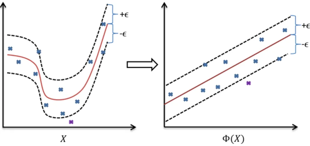
The formulation of the support vector optimisation problem considered up to now assumes a linear relationship between the inputs and outputs in the training data. However, in many applications the relationship might be non-linear. A kernel function k can be introduced to implicitly map the training

points from the original input space X to a higher dimensional feature space

Φ(X)such that a linear relationship between the variables exist inΦ(X). The

support vector expansion of the target function for linear regression is then applicable in the feature space, as illustrated in Figure 3.6.

The linear support vector expansion given by equation (3.20) is expanded by mapping the input data x from the original space X to some feature space

Figure 3.6: A nonlinear input-output relationship in the original space X on the left is mapped into the feature space Φ(X) on the right where the relationship becomes linear. The feature space is typically in a higher dimension. However, for illustration purposes, it is shown in the same dimension as the feature space. Redrawn from Thissenet al.(2003).

(38)

CHAPTER 3. DATA-DRIVEN MODELLING 28

Φ(X). The solution of equation (3.20) changes to

f(x) = n X i=1 (αi−α∗i)k(xi,x) +c, (3.32) where k(x,y) =hΦ(x1),Φ(x2)i for x1,x2 in X. (3.33)

As seen in equation (3.32), it is no longer required to find the flattest function in the input space X, but rather to find the flattest function in the feature

spaceΦ(X). In SVR formulations, linear, polynomial, radial basis and sigmoid

kernel functions are commonly used. These kernel functions are defined as follows:

linear: k(x1,x2) = x1Tx2, (3.34)

polynomial: k(x1,x2) = (γx1Tx2+r)v, (3.35) radial basis: k(x1,x2) = exp(−γkx1−x2k2), γ >0, (3.36) sigmoid: k(x1,x2) = tanh(γx1Tx2+r). (3.37) Variablesγ,vandrare kernel-specific hyperparameters. The aim of optimising

the SVR model’s ability to generalise input data well is achieved by fine-tuning the model and its parameters (Bray and Han, 2004). Therefore, choosing an optimal model structure and corresponding hyperparameters, as well as values for and C, is important when training an SVR model to fit a given dataset

(Granata et al., 2016).

3.3.3

Advantages and drawbacks

As mentioned in Section 3.2, a significant advantage of a support vector regres-sion model lies in the formulation of its convex objective function, which en-sures that the global optimum will always be found. Furthermore, the penalty parameter C suppresses outliers within a dataset and therefore ensures a

gen-eralised model as well as robustness to noise (Bray and Han, 2004). According to Raghavendra and Deka (2014), another main advantage of SVR is the si-multaneous minimisation of model complexity and prediction error by using the kernel trick.

The main drawback of SVR is the heuristic process of determining the optimal kernel function and corresponding hyperparameters, as well as the optimal val-ues for andC (Raghavendra and Deka, 2014). This is usually determined by

a grid search algorithm, which considers all possible parameter combinations, trains the SVR model on each combination and evaluates its performance us-ing a metric such as K-fold cross validation. The optimal parameters are then

chosen by determining the combination with the lowest cross-validation error. This can be a time-consuming and computationally expensive task, especially for larger grids.

(39)

CHAPTER 3. DATA-DRIVEN MODELLING 29

3.4

Neural networks

Neural networks are parallel-distributed information systems consisting of a number of densely interconnected processing elements that work in unison to solve a specific problem (Yaseenet al., 2015). A neural network can be designed

for different types of applications, including pattern recognition and data clas-sification. It has been extensively used for hydrological modelling purposes and time series forecasting applications, and has been found to be especially suitable when the underlying functions that describe complex phenomena are unknown (Maier and Dandy, 2000).

3.4.1

Model formulation

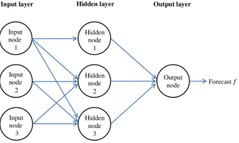
A neural network contains a set of interconnected nodes that receive, process and send information to one another over weighted connections. These nodes are grouped in different layers. As illustrated in Figure 3.7, input values enter the model through the first layer (the input layer). The data is then fed forward through successive hidden layers until it reaches the final layer (the output layer). The hidden layers enable the neural network to learn complex relationships between data (Solomatineet al., 2008). A neural network can be

single layered, bilayered or multilayered, depending on the number of hidden layers.

Neural networks are further classified as feed-forward or recurrent, based on the direction of information flow and processing between nodes. Feed-forward neural networks allow information to travel in only one direction: from the input layer to the output layer. Recurrent neural networks allow information to travel in both directions. Even though recurrent networks have shown to be very useful in time series applications, they are difficult to train and have a slower processing speed in comparison with feed-forward networks (Remesan

(40)

CHAPTER 3. DATA-DRIVEN MODELLING 30 and Mathew, 2014; Masters, 1993). According to Khotanzad et al. (1997),

feed-forward networks have performed well compared to recurrent networks in many practical applications. Taver et al. (2015) also performed a study

on the comparison of feed-forward and recurrent networks for non-stationary hydrological modelling and concluded that no model outperformed the other. Feed-forward networks will therefore be the focus of this study.

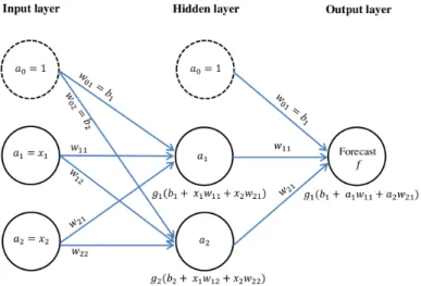
A widely studied and used feed-forward neural network model in hydrology is the multilayer perceptron (MLP). An MLP consists of an input layer, at least one hidden layer and an output layer. Weights determine how inputs are related to outputs and are assigned based on an input’s relative importance to other inputs. For each node, an output is determined by calculating the sum of its weighted inputs, and applying a nonlinear transformation called an activation function. Furthermore, each layer contains an additional input with a numerical value of 1, for which its connected weight is known as a bias.

Consider the single hidden layered MLP given in Figure 3.8. Let i, j and k

represent the position of each node in the input, hidden and output layers, respectively. Feed-forward computations are performed by first multipyling each input value xi from the input layer with a set of connected weights wij connecting the input layer with the hidden layer. These weighted values are then summed with the bias bj and transformed by the hidden layer activation function gj, such that an outputgj(bj+P_ixiwij)is obtained for the jth node in the hidden layer. Similarly, each output from the hidden layer is multiplied by the weights wjk connecting the hidden layer with the output layer, summed

Figure 3.8: A single layered MLP. Feed-forward computations are performed by multipyling each input valuexiwith a set of connected weightswij, connecting the input layeriwith the

hidden layerj. These weighted values are then summed with the bias bj and transformed

by the hidden layer activation function gj, to obtain an output gj(bj+P

ixiwij)for the jth _{node in the hidden layer. A similar procedure is followed from the hidden layer to the}

(41)

CHAPTER 3. DATA-DRIVEN