w or k i ng pa p ers
11 | 2011
April 2011
The analyses, opinions and fi ndings of these papers
represent the views of the authors, they are not necessarily those of the Banco de Portugal or the Eurosystem ASSESSING MONETARY POLICY IN THE EURO AREA: A FACTOR-AUGMENTED VAR APPROACH
Rita Soares
Please address correspondence to Banco de Portugal Av. Almirante Reis 71, 1150-012 Lisboa, Portugal;
BANCO DE PORTUGAL Av. Almirante Reis, 71 1150-012 Lisboa
www.bportugal.pt
Edition
Economics and Research Department
Pre-press and Distribution
Administrative Services Department Documentation, Editing and Museum Division Editing and Publishing Unit
Printing
Administrative Services Department Logistics Division Lisbon, April 2011 Number of copies 170 ISBN 978-989-678-078-4 ISSN 0870-0117 (print) ISSN 2182-0422 (online)
Assessing Monetary Policy in the Euro Area:
a Factor-Augmented VAR Approach
∗Rita Soares
This version: April 2011
Abstract
In order to overcome the omitted information problem of small-scale vector autore-gression (VAR) models, this study combines the VAR methodology with dynamic factor analysis and assesses the effects of monetary policy shocks in the euro area in the period during which there is a single monetary policy. Using the factor-augmented vector autoregressive (FAVAR) approach of Bernanke et al. (2005), we summarise the information contained in a large set of macroeconomic time series with a small number of estimated factors and use them as regressors in recursive VARs to evaluate the impact of the non-systematic component of the ECB’s actions. Overall, our results suggest that the inclusion of factors in the VAR allows us to obtain a more coherent picture of the effects of monetary policy innovations, both by achieving responses easier to understand from the theoretical point of view and by increasing the precision of such responses. Moreover, this framework allows us to compute impulse-response functions for all the variables included in the panel, thereby providing a more complete and accurate depiction of the effects of policy disturbances. However, the extra information generated by the FAVAR also delivers some puzzling responses, in particular those relating to exchange rates.
Keywords: Factor models, European Monetary Union, monetary policy shock, vector autoregressions, factor-augmented vector autoregressions, impulse-response functions. JEL Classification: C32, E52, E58.
∗This work has resulted from a master thesis in “Monetary and Financial Economics”, performed at Technical University of Lisbon. I would like to thank my advisor Maximiano Pinheiro for his guidance and support. I am also grateful to Vítor Gaspar for his valuable comments. The views expressed in this paper are mine, along with any errors or mistakes.
1
Introduction
Following the seminal works of Bernanke and Blinder (1992) and Sims (1992), in-fluential papers have convincingly used vector autoregression (VAR) models with recursive identification schemes (henceforth recursive VARs) to identify and assess the effects of monetary policy innovations on macroeconomic variables. Indeed, since not all variations in central banks’ policy can be accounted for as a reaction to the state of the economy, VAR-based approaches focus on the non-systematic compo-nent of monetary policy rather than on the systematic one. The great appeal of using recursive VARs to estimate the effects of the unanticipated component of cen-tral banks’ actions seems to be their ability to deliver empirical credible responses of macroeconomic variables to a monetary policy shock without imposing burdensome restrictions on the dynamic structure of the model.
However, it is a fact that VAR models are small-scale models, based on a limi-ted information set, and this is often poinlimi-ted out as their major weakness for the analysis of monetary policy. Monetary policy makers actually monitor a very wide set of macroeconomic variables before deciding on the stance of their policy actions, and therefore omitting relevant information from the VAR analysis may hamper the validity of the empirical results, as this may lead to a situation in which VAR inno-vations will not, in general, span the space of the disturbances, and therefore the shocks cannot be deduced correctly from VAR innovations. Additionally, impulse-response functions can only be generated for the handful of variables included in the model, which represent a very small subset of the variables of interest to mone-tary authorities. However, due to degrees-of-freedom problems, it is not feasible to include a large number of time series in the model – as the number of unrestricted VAR coefficients increases in direct proportion to the square of the number of va-riables in the system – and therefore the problem of omitted vava-riables bias cannot be solved within the standard VAR framework.
Evidence emerging from a recent strand of empirical macroeconomic literature suggests that in order to properly capture the dynamics of the economy, significant advantages arise from resorting to models specifically designed to handle a large amount of information, the so-called dynamic factor models. Such models allow us to summarise the information contained in a large number of data series in a small number of estimated factors. Large-dimensional dynamic factor models have become popular in empirical macroeconomics in recent years, but the literature on dynamic factor analysis in economics goes back to Geweke (1977) and Sargent and Sims (1977). Currently, the estimation of dynamic factor models resorts mainly to two different methods: principal components and maximum likelihood. Regarding
the principal components method, two approaches have recently emerged for ex-tracting information from large data sets. The first is a time-domain analysis, stems from Stock and Watson (1998, 1999, 2002a, 2002b), and relies on the estimation of factors by static principal components. The second is a frequency-domain approach, was introduced by Forni et al. (2000, 2004, 2005), and relies on dynamic principal components. As regards the estimation of factors by maximum likelihood, in the domain of time, important contributions are those of Doz et at. (2006, 2007) and Reis and Watson (2007).
Bernanke et al. (2005) apply the Stock and Watson (1998, 1999, 2002a, 2002b) methodology to extract the factors that summarise the information present in a large data set and they include those factors in monetary VARs. The authors conclude that factor models are a natural solution to the degrees-of-freedom problem in the VAR analysis of monetary policy since they allow for conditioning of the VAR approach on rich information sets without giving up the statistical gains of restricting the analysis to a small number of regressors. The authors refer to their methodology as the factor-augmented VAR (FAVAR) approach. The amount of information that can be handled within the FAVAR is very large and hence the chance of misspecifying the econometric model used to assess the effects of monetary policy disturbances significantly decreases. Moreover, it makes possible to compute impulse responses of each of the variables included in the panel to the policy shock.
In this paper, we are interested in evaluating if the inclusion of factors in a VAR improves our understanding of the effects of euro area monetary policy shocks, either by changing the shape of the responses of main macroeconomic variables to those shocks, or by decreasing the uncertainty about such responses. Although there are already some applications of factor analysis to the assessment of the effects of monetary policy shocks in the euro area (e.g. Favero and Marcellino, 2005; Boivin, Giannoni and Mojon, 2009; and Blaes, 2009), none of the papers, at least to our knowledge, applies the FAVAR approach to the euro area figures as from the launch of the single monetary policy (their sample period typically begins before 1999 and, since there was not a single monetary policy at the time, some countries are used as proxies or, alternatively, the figures are obtained by aggregating the countries’ individual data), and therefore we hope to contribute towards filling the gap we have found in the literature. Our paper adds, by means of the innovative methodology applied by Bernanke et al. (2005) for the US, to the already ample and rich literature on the monetary transmission mechanism in the euro area (e.g. Peersman and Smets, 2003). Whenever possible we will try to compare, in qualitative terms, the results achieved for the euro area to those obtained by Bernanke et al. (2005) for the US.
With the purpose in mind of assessing if the extra information included in the econometric model really matters, we follow Bernanke et al. (2005) in using the Stock and Watson (1998, 1999, 2002a, 2002b) static principal components approach to extract factors from a data set comprising 150 macroeconomic time series for the euro area and then adding those latent factors as regressors in a VAR. We proceed by comparing our results to those of a standard five-dimensional VAR and conclude that the inclusion in the model of a very large set of variables, which potentially contain information about the monetary policy shock, succeeds in delivering respon-ses more easy to interpret from the economic point of view. In particular, we show that the small-scale VAR generates a price puzzle, i.e. a counterintuitive positive reaction of prices to an increase in the official interest rate and we also show that the decrease of real Gross Domestic Product (GDP) is very persistent, a fact which is inconsistent with long-run money neutrality. Conversely, in our FAVAR specifica-tions the price puzzle does not appear, which seems to corroborate the explanation of Sims (1992) that the price puzzle results from imperfectly controlling within the VAR for information that the central bank may have about leading indicators of inflation. Furthermore, the output response shows a consensual hump-shaped pattern. Another positive result is that the responses delivered by the different FAVAR specifications are more precise (have lower average standard deviations) than the responses delivered by the benchmark VAR.
Taking advantage of the special features of the FAVAR methodology, we proceed by computing impulse-response functions and variance error decomposition for a wider set of variables than those typically assessed in standard VARs. Our analysis delivers three main empirical results. First, the responses of the majority of the variables to the monetary policy shock are intuitive. For instance, an unexpected tightening in monetary policy results in a gradual decrease in industrial production, consumption expenditure, business sentiment indicators and money aggregates in the short run, before reverting to the baseline scenario as the effects of the shock fade out. Second, in line with the consensual finding in the literature that monetary policy affects the economy mostly through its systematic behaviour, we conclude that, apart from interest rates, the contribution of the policy shock for the variables’ forecast error variance decomposition is low. Third, the extra information generated by the FAVAR approach brings to light some striking results as regards the responses of exchange rates and the components of the Harmonised Index of Consumer Prices (HICP). In the first case, a rise in the official interest rate is associated with an initial depreciation of the euro, which is probably caused by the euro area monetary authority reacting to changes in foreign interest rates. In the second case, we find
that the intuitive negative response of inflation is strongly driven by the component energy and unprocessed food. In turn, although the magnitude is almost irrelevant, the response of the HICP excluding energy and unprocessed food reveals a price puzzle.
The paper is structured as follows. Section 2 describes the main methodological topics. In Section 3, the empirical implementation evolves in two steps. First, we present the main results, based on the estimation of impulse responses to the monetary policy shock and on the assessment of the fraction of the forecast error variance of the variables that is attributable to monetary policy disturbance. Second, we check our results for robustness to changes in some of the assumptions of the model. Section 4 concludes.
2
Econometric framework
In our study, we will follow Bernanke et al. (2005) in using the Stock and Watson (1998, 1999, 2002a, 2002b) principal components static approach, according to which the first principal components span the factor space even if the model is only appro-ximate. In this context, two important distinctions must be made.
The first is between the classical/strict/exact and the approximate formulation of a dynamic factor model. The exact formulation entails three restrictive assumptions on the idiosyncratic component of the variables: they have to be cross-sectionally independent, serially independent and uncorrelated with the common factors. In its turn, the approximate factor model allows for some heteroskedasticity and limited dependence of the idiosyncratic components (serially and cross-sectionally), as well as for some moderate correlation between the latter and the factors (see, for instance, Stock and Watson (1998, 2002a) and Bai and Ng, 2002).
The second is between the static and the dynamic representation of a dynamic factor model. In the latter, factors can enter with lags or leads in the data generating process of each variable. In the former, factors appear without any lags, which means that factors only have a contemporaneous effect on the variables.1 The static approach relies on the time-domain forecasting method of Stock and Watson (1998, 1999, 2002a, 2002b), whose estimates are based on contemporaneous covariances 1In order to make this terminology clear – and it might at first seem quite misleading – it is
required to note that the term static in a dynamic factor model refers to the static relationship between the common component and the variable; however, the common component itself can be a dynamic process, i.e. can capture arbitrary lags of some fundamental factors. As Forni et al. (2004) assert, when all variables are “hit” by the common shocks at the same time, the model is called static; when different variables are “hit” by different lags of the common shocks, the model is called dynamic.
only, meaning that they do not exploit the potential information contained in the leading-lagging relations between the elements of the panel. The authors show that when both the number of variables and the time dimension tend to infinity, the space of factors is consistently estimated by static principal components, even in an approximate factor model with factor loadings constant and idiosyncratic errors that are serially and (weakly) cross-sectionally correlated. In its turn, the dynamic method is mainly due to Forni et al. (2000, 2004, 2005) and Doz et al. (2006, 2007). The latter use a time-domain approach, estimated by a Gaussian maximum likelihood method, while the former rely on a frequency-domain method, estimated by dynamic principal components, based on the dynamic covariance structure of the data.
2.1
Time domain analysis of the dynamic factor model
Factor models represent the vector of N time series as a linear combination of two unobserved components, a common component, driven by a small number of factors, plus an idiosyncratic component. LetXtbe theN×1vector of stationary zero mean
variables under analysis, observed for timet = 1,2, ..., T. In the general formulation of a dynamic factor model, each element of the vector Xit = [X1t, ..., XN t]0, for
i= 1,2, ..., N, can be represented as:
Xit =λi(L)ft+eit (1)
whereftis theq×1vector of common factors(q N), whose dynamic effects onXit
are grouped inλi(L) = λi0+λi1L+λi2L2+...+λipLp, lag polynomials in nonnegative
integer powers ofL (where each λi is a N ×q matrix), and et = [e1t, ..., eN t]0 is the
N×1 vector of idiosyncratic disturbances. An alternative formulation of the model is: Xt = ΛFt+et (2) where Ft = [ft0, f 0 t−1, ..., f 0 t−p]
0 is r ×1, so that now r = (p+ 1)× q factors drive
the variables, but the factors have only a contemporaneous effect on Xt, with
loa-dings grouped in the N ×r matrix Λ = [λ0, λ1, ..., λp], the i-th row of Λ being
Λi = [λi0, ...λip]. Since the association between factors and variables is only
contem-poraneous, the dynamic factor model is in its static formulation.
Note that we cannot estimate Ft, but instead we can estimate the
common-factor space, i.e. a r-dimensional orthogonal vector whose entries span the same linear space as the entries of Ft. In fact, the factors are not identified because for
any invertibler×r matrix G, Equation (2) can be rewritten as
Xt = ΛGG−1Ft+et= ΨPt+et (3)
wherePtis an alternative set of factors. In spite of the identification problem (which
complicates the structural interpretation of the factors), Pt is just a linear
trans-formation of Ft, and therefore both are equivalent in summarising the information
contained in Xt.
In the classical or exact formulation of the factor model, the idiosyncratic com-ponents are assumed to be serially and cross-sectionally independent and the factors are assumed to be serially uncorrelated. Moreover, E[Fte0t] = 0, i.e. the factors and
the idiosyncratic components are required to be mutually orthogonal. However, the assumptions of the exact model may be viewed as too restrictive and even unrealistic in economic terms.
Stock and Watson (1998) developed a nonparametric approach for the time do-main analysis of the dynamic factor model based on the static principal components of Xt.2 The authors show, under the finite lag assumption and some additional
technical assumptions, that the common space spanned by the dynamic factors Ft
can be estimated consistently by the principal components of theT ×T covariance matrix ofXt, even if some of the restrictive assumptions of the classical model are
neglected. In this way, consistency of the estimators requires the factors Ft to be
orthogonal, i.e. uncorrelated with each other, but they can be correlated in time and can also be weakly correlated with the idiosyncratic component. In this approxi-mate factor model, limited dependence of the idiosyncratic disturbances is allowed in both dimensions.
The starting point in the Stock and Watson (1998) approach is the estimation of the factorsFt and the loadings Λ. Let the estimatorsFbt be the minimisers of the
least squares criterion:
VN,T(F,Λ) = (N T)−1 N X i=1 T X t=1 (Xit−ΛiFt)2 (4)
where F = [F1, ..., Ft, ..., FT]0 and Λi is the i-th row of Λ, subject to the constraint
T−1F0F =T−1PT
t=1FtFt0 =Iq.
Under the hypothesis of k common factors, Stock and Watson (1998) show 2This means that the correlation structures and distributions of the idiosyncratic terms and the
factors and the precise lag structure by which the factors enter are not specified parametrically (Stock and Watson, 1998).
that the least squares estimators of the factors Fb = [Fb1, ...,Fbt, ...,FbT]0 are the
k eigenvectors corresponding to the k largest eigenvalues of the T × T matrix
(N)−1PN
i=1X ∗
iX∗0i, where Xi∗ = [Xi1, ..., XiT]0. The least squares estimators of
the loadings are then obtained from a linear regression (OLS) of the variables on the estimated factors. Moreover, the least squares estimators of the loadings are the k eigenvectors corresponding to the k largest eigenvalues of the N ×N matrix
(T)−1PT
t=1XtX 0
t. The authors prove that when the assumed number of factors, k,
is equal to the true number, r, the entries of Fbt span the same linear space as the
entries of Ft. When k > r, there are k −r estimated factors that are redundant
linear combinations of the elements of Ft. When k < r, consistent estimation of
a subspace of dimension k is preserved, because of the orthogonality hypothesis. Finally, the estimator of the common component can be obtained as bxt=ΛbFbt and,
consequently, the estimator of the idiosyncratic component is bet=Xt−bxt.
In order to determine the number of factors needed to properly capture the effects of monetary policy disturbances, we will follow Bernanke et al. (2005) in using the Bai and Ng (2002) IC2(k) criterion, the one that is commonly used for
the determination of the number of factors both when US large data sets and euro area large data sets are considered:
IC2(k) = ln VN,T(Fb(k),Λb(k)) +k N +T N T ln (min{N, T}) (5)
whereVN,T(Fb(k),Λb(k))denotes the sum of squared residuals from ak-factor model, as
defined in Equation (4), withFb(k)and Λb(k)being the estimated factors and loadings.
The information criterion reflects the trade-off between goodness-of-fit, on the one hand, and overfitting, on the other. The first term on right-hand side of Equation (5) shows the goodness-of-fit, as if the number of factors increases, the variance of the factors also increases and the sum of squared residuals decreases. Hence, the information criterion has to be minimised in order to determine the number of factors. The penalty of overfitting, which is the second term on the right-hand side of Equation (5) is an increasing function ofN and T.
2.2
The factor-augmented VAR
2.2.1 The model
LetXtdenote anN×1vector of economic time series,Yta vector ofM×1observable
macroeconomic variables that constitutes a subset of Xt and Ft a k×1 vector of
unobserved factors that capture most of the information contained inXt. According
transition equation: " Ft Yt # = Φ∗(L) " Ft−1 Yt−1 # +υt ⇔Φ(L) " Ft Yt # =υt (6)
whereΦ(L) =I−Φ∗(L)L =I −Φ1L−...−ΦdLd is a conformable lag polynomial
of finite orderd in the lag operator L, Φj (j = 1, ..., d)is the coefficient matrix and
vt is an error term with mean zero and covariance matrixQ. Equation (6) is a VAR
model, which may contain a priori restrictions as in the VAR literature, but which includes both observable and unobserved variables. Bernanke et al. (2005) refer to Equation (6) as a factor-augmented vector autoregression, or FAVAR.
Since the factors are unobserved, Equation (6) cannot be estimated directly. However, we can interpret the factors, in addition to the observed variables, as the common forces driving the dynamics of the economy. For concreteness, we can assume that the relation between the “informational” time series Xt, the observed
variablesYtand the factors Ft can be summarised in the following (static)
represen-tation of a dynamic factor model:
Xt= ΛfFt+ ΛyYt+et (7)
where Λf is a N ×k matrix of factor loadings, Λy is N ×M and e
t is the vector
ofN×1error terms weakly cross-sectionally and serially correlated and with mean zero. The specification of the dynamic factor model à la Stock and Watson (1998) implies that Xt does not depend on the lagged values of Ft, only on the current
ones (static representation of the dynamic factor model). Since we assume that M+k N, the amount of information that can be handled in a FAVAR increases significantly in comparison to standard VAR models.
2.2.2 Identification of the factors
For the estimation of the FAVAR model (6)-(7) we will follow the two-step principal components approach used in Bernanke et al. (2005), which is a nonparametric way of estimating the common space spanned by the factors of Xt, i.e. C(Ft, Yt).3,4 In
3Bernanke et al. (2005) also tried an alternative approach making use of Bayesian likelihood
methods and Gibbs sampling to estimate the factors and the dynamics simultaneously. The authors conclude that the advantages of using this procedure (more computationally burdensome) are modest, and therefore we will only make use of the principal components approach.
4We will use the same terminology as in Bernanke et al. (2005) and will refer to C(F
t, Yt)as the common space spanned by the factors ofXt, i.e. both by the latent factorsFtand the observed factorsYt. Although it might seem quite abusive to classifyYtalso as a factor, the rationale behind this terminology is that both Ft and Yt have pervasive effects throughout the economy and are
the first step, C(Ft, Yt) is estimated using the first k+M principal components of
Xt; in the second step, Equation (6) is estimated with Ft replaced by Fbt.
We will follow the work of Bernanke et al. (2005) and will not exploit the fact that Yt is observable in the first step. However, as shown in Stock and Watson (2002b),
whenN is large and the number of principal components used is at least as large as the true number of factors, the principal components consistently recover the space spanned by bothFt and Yt. In this way, obtaining Fbt implies determining the part
ofCb(Ft, Yt)that is not spanned byYt, i.e. by removingYtfrom the space covered by
the principal components. This will be done in the second step, relying on a specific identifying assumption that exploits the different behaviour of the several variables included in Xt.5 For concreteness, the matrix Xt is divided into slow-moving and
fast-moving series. The former are those variables that are assumed to be prede-termined as of the current period, i.e. that do not respond contemporaneously to unanticipated changes in monetary policy (e.g. real variables). The latter are those variables that are allowed to respond contemporaneously to policy shocks (e.g. asset prices). In order to remove the direct dependence of Cb(Ft, Yt) on Yt, the foothold
is to obtain Cb∗(Ft) as an estimate of all the common components other than Yt.
Since slow-moving variables are assumed not to be affected contemporaneously by Yt, Cb∗(Ft) is obtained by extracting principal components from this set of
varia-bles. Afterwards, the estimated common componentsCb(Ft, Yt)are regressed on the
estimated slow-moving factors Cb∗(Ft) and on the observed variables Yt:
b
C(Ft, Yt) =aCb∗(Ft) +bYt+ut (8)
Finally,Fbtis calculated asCb(Ft, Yt)−bbYtand the VAR inFbtandYt is estimated:
b Ψ(L) " b Ft Yt # =εt (9)
whereΨ(b L) =Ψb0−Ψb1L−...−ΨbdLd is a matrix of orderdin the lag operatorL,Ψbj (j = 0,1, ..., d)is the coefficient matrix andεt is the vector of structural innovations
within the diagonal covariance matrix.
thus considered common components of all variables entering the data set.
5In a more recent paper, Boivin, Giannoni and Mihov (2009) impose the constraint that Y
tis one of the common components in the first step, guaranteeing that the estimated latent factorsFbt recover the common dynamics not captured byYt. The authors compare their methodology with that of Bernanke et al. (2005) and conclude that the results are similar.
2.2.3 Identification of the VAR
For the identification of the macroeconomic shocks, we will follow Bernanke et al. (2005) assuming a recursive structure where the factors entering Equation (6) respond with a lag (i.e. do not respond within the period, here a month) to unan-ticipated changes on the monetary policy instrument.
The recursiveness assumption makes use of the Cholesky decomposition of the variance-covariance matrix of the estimated residuals, a simple algorithm for splitting a symmetric positive-definite matrix into a lower triangular matrix multiplied by its transpose. The Cholesky decomposition implies a strict causal ordering of the va-riables in the VAR: the variable positioned last responds contemporaneously to all the others, while none of these variables respond contemporaneously to the variable ordered last; the next-to-last variable responds contemporaneously to all variables except the last, whereas only the last variable responds contemporaneously to it. A popular identifying assumption in VAR studies of the monetary transmission me-chanism – which Bernanke et al. (2005) used for the identification of the FAVAR – is that the monetary policy shock is orthogonal to the variables in the policy rule, in the sense that economic variables in the central bank’s information set do not respond contemporaneously to realisations of the monetary policy shock (i.e. there are some variables that are predetermined to the policy shock). As in Bernanke et al. (2005), we will assume a Cholesky identification scheme in which the policy variable, in our case the European Central Bank (ECB) policy rate,6 is ordered after the factors, output and prices and will treat its innovations as the policy shocks.
6Throughout the text, we will always refer to the policy variable as the ECB policy rate.
Nevertheless it should be clarified that, in the empirical exercise, we have followed the strategy usually used in the VAR literature and have preferred to use an effective rate instead of the target rate itself. In this way, we have considered the Euro OverNight Index Average (EONIA) as a proxy for the “effective policy rate”. The EONIA is the effective overnight reference rate for the euro area and is computed as a weighted average of all overnight unsecured lending transactions undertaken in the interbank market, initiated within the euro area by the banks belonging to the contributing panel. The EONIA is the interbank rate that follows more closely the ECB policy rate and one of the ECB’s aims is to contribute to the smooth path of this market rate. In our sample period, the EONIA was, on average, five basis points higher than the ECB policy rate. This reduced spread reinforces our idea that the EONIA rate might be the best proxy for the policy variable.
3
Empirical analysis
3.1
The data
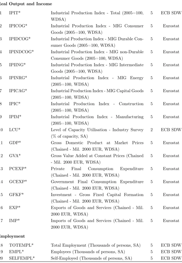
Our data set consists of a balanced panel of 150 monthly macroeconomic time series for the 16-country euro area from 1999:1 to 2009:3.7 The choice of the starting date reflects our desire to maximise the sample length while considering that the assessment of a single monetary policy in the euro area only makes real sense after the launch of the euro. The macroeconomic series were chosen from the following categories: real output and income; employment; prices; exchange rates; interest rates; stock prices; money and credit aggregates; industrial new orders and turnover; retail sales and turnover; building permits; balance of payments and external trade; confidence indicators; and some foreign variables (US, Japan and United Kingdom’s GDP, inflation and interest rates). Appendix A lists all the series in the data set and their transformation.
The data were processed in five stages. First, as seasonal patterns are often so large that they may hide other characteristics of the data that are of interest for the analysis of economic trends, the series were seasonally adjusted, i.e. the seasonal effects of the series were estimated and removed. The approach we used relies on a multiplicative decomposition through X-12-ARIMA, for all positive series, and on an additive decomposition for the remaining series.
Second, as we intended to work with a balanced panel of monthly series, we had to disaggregate the quarterly series into monthly ones, using the Eurostat statisti-cal software Ecotrim. In the econometric and statististatisti-cal literature, two univariate approaches to disaggregate economic series observed at low frequency into compa-tible higher frequency data have been generally followed: (i) methods which do not involve the use of related series and (ii) methods which make use of the information coming from related indicators observed at the desired higher frequency (for a re-view of the methods, see Di Fonzo, 2003). Since the first approach only comprises purely mathematical methods, we have chosen the latter as the most interesting for our purposes. However, instead of selecting a small set of variables to help in the disaggregation of each of the quarterly variables (e.g. the GDP is usually di-saggregated using as a related indicator the industrial production index), we have followed Angelini et al. (2006) in exploiting a disaggregation method that makes use of the factors estimated from a large data set. For concreteness, we have modelled 7We have used final, i.e. revised data and not real-time data, which means that at the time the
ECB has decided on the stance of the monetary policy, the figures it has used (unrevised data) might have been different from ours.
the large amount of information available in the monthly time series by means of a dynamic factor model (using a principal-component-based estimation procedure as described in Section 2.1) and have used the estimated factors as related indicators for the disaggregation process. Angelini et al. (2006) demonstrate that this factor approach generally outperforms more standard disaggregation methods if (i) there is a large number of explanatory variables for the variable to be disaggregated, (ii) the variables to be used for factor extraction have a limited idiosyncratic component and (iii) there is a limited measurement error for both the explanatory variables and the variable to be disaggregated in the periods in which the latter cannot be observed. For the case when related indicators are available, several restrictions on the data generating process of the regression error have been proposed. We have followed the method proposed by Litterman (1983), according to which the model is estimated in first differences and the regression error follows anAR(1) process.8,9 Third, the series were transformed to account for stochastic or deterministic trends. The decision to take logarithms and/or first differences was based on unit root tests, so that the transformed series are approximately stationary. In general, first differences of logarithms were taken for all nonnegative series that were not already in rates or percentage units. The same transformation, including degree of differencing, was in general applied to all the series included in a specific group (e.g. first difference of logarithms was taken for all price indexes).
Fourth, following the common procedure in this type of analysis (e.g. Stock and Watson, 2005), the transformed seasonally adjusted series were screened for outliers and observations with deviations from the median exceeding six times the interquartile range (in absolute terms) were replaced by the median value of the preceding five observations.
Finally, since the different scales of the time series could impair factor extraction, all “informational” series used to compute the factors were standardised to have mean zero and unit variance. The VAR/FAVAR estimation, however, was conducted using non-standardised observed variablesYt.
8Alternative methods have been proposed by Chow and Lin (1971) and Fernández (1981). In
the former, the regression error follows anAR(1)process and the model is estimated in levels while in the latter the disturbance term follows a random walk.
9More specifically, we have followed the steps detailed next: first, as the theory on dynamic
factor models assumes that the set of “informational” variables contains only I(0) series, we have transformed the monthly series to induce stationarity; second, as the estimated factors have mean zero and unit variance but the variables to disaggregate do not, we have followed Di Fonzo (2003) in performing the following transformation to the latter: 3 ln(yt)−3 ln(3), yt being the variable to be disaggregated and 3 being the number of months in a quarter; and third, as the Litterman (1983) disaggregation method applies first differences both to the explanatory variables and the dependent variable, we have used as explanatory variables the accumulated factors and not the factors themselves.
3.2
Empirical implementation
As the baseline scenario of our FAVAR empirical application, we assume that the only observable variable is the policy instrument, i.e. the ECB policy rate (Rt), so
that Yt =Rt. However, we follow Bernanke et al. (2005) in defining an alternative
specification in which the output (GDP) and the inflation (HICP) are also included inYt, so thatYt= (GDPt, HICPt, Rt). In addition, we consider a second alternative
formulation in which we add a nominal effective exchange rate (NEER) to the set of observable variables, so that Yt = (GDPt, HICPt, Rt, N EERt). We proceed by
comparing the results of the three FAVAR specifications with those of a small-scale standard VAR model based on the ECB commodity price index, the real GDP, the HICP, the ECB policy rate and the nominal effective exchange rate.10 Standard likelihood ratio tests are used to determine the lag-order of the models. The VAR turns out to be of order three, while the baseline FAVAR and both the two alterna-tive FAVARs turn out to be of order two. All models are estimated with a constant and a linear trend. Finally, we set the number of factors in the FAVAR specifica-tions as seven, based on the information criterion IC2(k) proposed in Bai and Ng
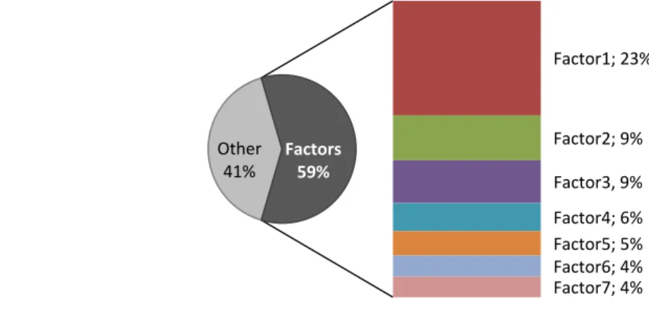
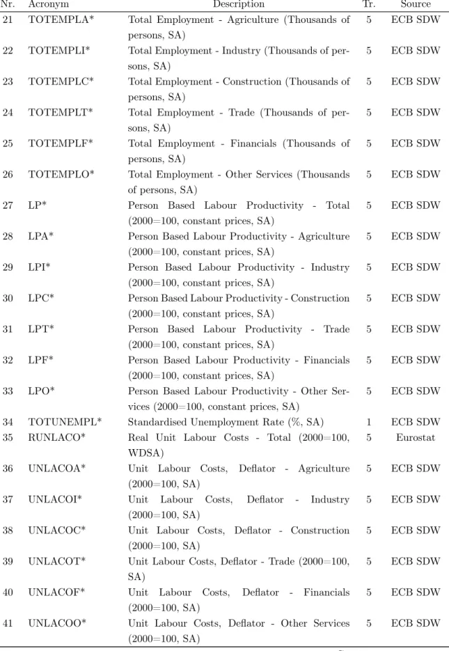
(2002). Together, these seven factors explain 59 per cent of the joint-variance of the 150 variables included in our large data set (with the first factor explaining around 23 per cent of the variation on the data set and the first five factors explaining about half of the total variance, as depicted in Figure 1). A tentative interpretation of the factors is performed in Appendix B.
Figure 1: Cumulated share of variance explained by the first seven static factors
Factor1; 23% Other 41% Factor1; 23% Factor2; 9% Factor3, 9% Factor4; 6% Factor5; 5% Factors 59% Other 41% Factor1; 23% Factor2; 9% Factor3, 9% Factor4; 6% Factor5; 5% Factor6; 4% Factor7; 4% Factors 59%
10In the literature we can find both VARs where the nominal effective exchange rate is used
and VARs where the real effective exchange rate is preferred. We have decided to use the nominal rate, just because it would also be our choice if we would choose instead a bilateral exchange rate (e.g. vis-à-vis the US dollar). Nevertheless, we have compared our VAR with one including the real effective exchange rate and the results are roughly similar, both in terms of the shape and the magnitude of responses.
We divide the analysis of the results into three stages. First, we compare the impulse responses of the small-scale VAR with those of the FAVARs, showing that adding factors to benchmark VARs resolves the price puzzle. Second, we describe the impulse-response functions of several variables included in the FAVARs. Finally we look at the variance decomposition of the prediction errors. Afterwards, we check our results for robustness to changes in some of the assumptions of the model.
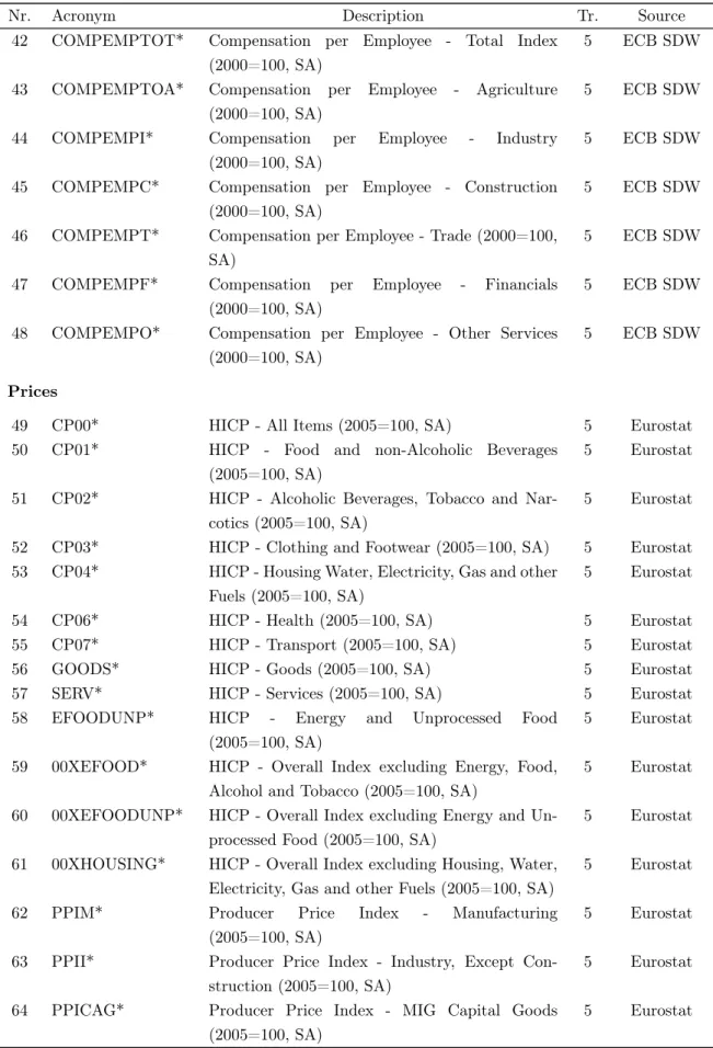
3.2.1 VARs versus factor-augmented VARs
Figure 2 displays the impulse-response functions computed both for the benchmark VAR model and the three FAVAR specifications. The identification of the monetary policy shock is obtained using a standard Cholesky decomposition. In the baseline and the first alternative FAVAR models, the policy interest rate is ordered last. In the benchmark VAR and in the second alternative FAVAR formulation, the po-licy rate is ordered before the nominal effective exchange rate, with this variable ordered last. The underlying assumption is that monetary policy shocks have no contemporaneous impact on output, prices and the factors, but they may affect the exchange rate immediately. However, the short-term key interest rate does not res-pond contemporaneously to changes in the nominal effective exchange rate. This is a common hypothesis in standard VAR literature for the European Monetary Union (e.g. Peersman and Smets, 2003). Responses of the GDP and the HICP are pre-sented in percentage deviations from the baseline (i.e. non-disturbed) scenario, while interest rate responses are expressed in percentage point deviations. In the bench-mark VAR model, a one-standard-deviation monetary policy shock corresponds to a 13 basis points increase in the official interest rate, which is somewhat greater than in the FAVAR models: 10 basis points in our preferred specification and 9 basis points in both alternative ones.11 In all models, we standardise the monetary policy
shock to correspond to a 25-basis-point innovation (hike) in the official interest rate. As Figure 2 displays, the benchmark VAR model suffers from what is commonly known in the literature as a price puzzle, i.e. the counterintuitive positive reaction of prices to an increase in the official interest rate, in the short term. Moreover, the response of real GDP is very persistent, which is not in line with the usual finding in the literature that the output follows a hump-shaped pattern in response to a monetary policy disturbance, before slowly returning to baseline. As Bernanke et al. (2005) highlight for the US, the persistence of the output response is inconsistent with long-run money neutrality.
11It must be noticed that for the benchmark VAR model, our monetary policy disturbance is
well below the estimate of 30 basis points obtained by Peersman and Smets (2003) for the period 1980-1998, before the launch of the euro.
Figure 2: Impulse responses to a monetary tightening shock ‐0.80 ‐0.60 ‐0.40 ‐0.20 0.00 0.20 0 12 24 36 48 perc. GDP ‐0.25 ‐0.20 ‐0.15 ‐0.10 ‐0.05 0.00 0.05 0 12 24 36 48 perc. HICP ‐0.40 ‐0.20 0.00 0.20 0.40 0 12 24 36 48 p.p. Interest rate
Benchmark VAR Baseline FAVAR (Y=R; k=7)
Alternative FAVAR 1 (Y=GDP, HICP, R; k=7) Alternative FAVAR 2 (Y=GDP, HICP, R, NEER; k=7)
Notes: Deviations from the baseline in percentage, except for the interest rate, for which the ordi-nate is in percentage points. Number of months after the monetary policy shock in the abscissa.
Conversely, in all FAVAR specifications the price puzzle does not appear. Accor-ding to the explanation given by Sims (1992), the price puzzle might be caused by the misspecification of the monetary authority’s information set, which means that the puzzle results from imperfectly controlling within the VAR for information that the central bank may have about leading indicators of inflation. In other words, the explanation for the price puzzle is that the central bank preemptively raises interest rates in anticipation of future inflation; however, in this case, what has been labelled as a non-anticipated policy shock contains, in fact, a fraction of the systematic response of the monetary authority to higher expected inflation. To the extent that the additional information processed by the central bank is not reflected in small-scale VARs, the measurement of policy innovations is likely to be “conta-minated”: what appears to the econometrician to be a policy shock is, in fact, the response of the central bank to the extra information not included in the VAR. Sims (1992) explanation of the price puzzle has led to the practice of including commodity price indexes into VARs, to attempt to control for future inflation. However, in our small VAR for the euro area, it does not seem to be enough. In this context, the disappearance of the price puzzle within the FAVAR approach might indicate that our estimated factors, which summarise the information contained in a large data set of macroeconomic variables, properly capture the information about prices that the central bank effectively monitors when deciding on monetary policy. Further-more, the response of output is more in line with theory, showing a hump-shaped pattern and eventually returning towards zero as the effects of the shock fade out. The maximum impact on output occurs almost 22 months after the shock and is 0.55 per cent in the baseline FAVAR model and 0.48 per cent and 0.57 per cent in the two alternative versions. Also the impulse responses of the short-term interest rate are consistent with theory. The interest rate initially reflects its own shock and falls in the first 24 months and then returns to baseline.
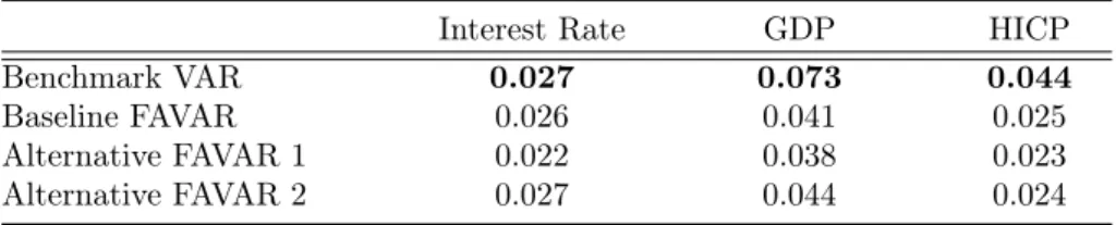
The analysis has to be completed with the comparison of the precision of res-ponses. Table 1 presents the standard errors for the responses of interest rate, GDP and inflation to a one-standard-deviation monetary policy innovation, for each of the four models under analysis. It must be noticed that, as Bernanke et al. (2005) highlight, the two-step approach used to estimate the FAVARs suffers from “genera-ted regressors” in the second step. In this way, the standard errors delivered by the usual econometric packages tend to underestimate the degree of uncertainty of res-ponses, since they are computed on the assumption that the regressors included in the VAR are observed, which is not our case, as the factors are latent variables. To overcome this caveat, the standard deviations for the FAVARs (and, for comparison purposes, also for the benchmark VAR) were calculated using a standard bootstrap procedure, with 5,000 replications, which accounts for the uncertainty in the fac-tor estimation. The results depicted in Table 1 confirm that the benchmark VAR presents the lowest precision of responses for any of the three variables (but mostly for output and inflation). The additional information delivered by the factors seems to reduce the uncertainty of responses, the first alternative FAVAR being the one showing lower standard deviations, followed by our baseline FAVAR specification.
Table 1: Uncertainty of impulse-response functions
Interest Rate GDP HICP
Benchmark VAR 0.027 0.073 0.044
Baseline FAVAR 0.026 0.041 0.025
Alternative FAVAR 1 0.022 0.038 0.023
Alternative FAVAR 2 0.027 0.044 0.024
Notes: Standard errors for the responses to a Cholesky (degrees-of-freedom adjusted) one-standard-deviation monetary policy innovation (average over 60 periods after the shock). Figures in bold represent the highest dispersion among the four models.
3.2.2 FAVAR impulse-response functions
Following Equation (9) in Section 2.2.2, the impulse responses of the estimated factors and of the variables observed included in Yt are computed as follows:
" b Ft Yt # =bδ(L)εt (10)
where bδ(L) = [Ψ(b L)]−1 =bδ0−bδ1L−...−bδhLh is a matrix of polynomials in order
Equation (7), the estimator ofXt is Xbt =ΛbfFbt+ΛbyYt, impulse-response functions
of each variable included in Xt can be obtained as follows:
XtIRF =hΛbf Λby i " b Ft Yt # =hΛbf Λby i b δ(L)εt (11)
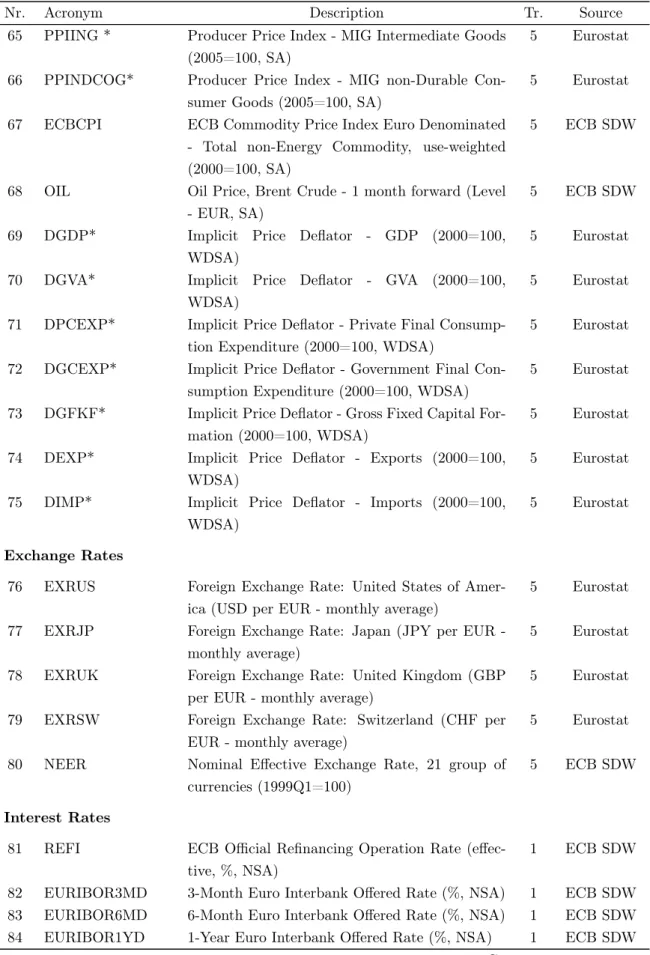
Figures 3 to 5 depict the impulse responses of a subset of 20 key variables to the monetary policy innovation for our baseline and the two alternative FAVARs, respectively. The corresponding 90 per cent confidence intervals (dashed lines) were calculated using a standard bootstrap procedure with 5,000 iterations, as explained earlier. It must be stressed that although we only display responses for a small subset of variables, impulse responses can be generated for all the variables included in the panel making use of Equation (11). This is so because all the variables included in the data set can be represented as linear combinations of the estimated factors (Fbt
and Yt) plus idiosyncratic noise. The responses in Figures 3 to 5 are very similar
and have in general the intuitive sign and magnitude. However, there are also some counterintuitive responses for some variables.
An unexpected tightening in monetary policy results in a gradual decrease in industrial production, which reaches its maximum effect after around two years, before reverting to the baseline scenario. The shape of the response is similar to that of the real GDP, but the magnitude is higher, since an unexpected 25-basis-point increase in the policy rate has a maximum impact on industrial production of more than one per cent in all the three formulations. When we split the analysis of the industrial production index, we find out that this strong response is mainly explained by the behaviour of durable consumer goods, since the impact of the monetary policy disturbance on nondurable consumer goods is rather more modest. In its turn, capacity utilisation reaches its maximum decline roughly two years after the monetary tightening, after which it eventually returns towards zero. The reaction of consumption expenditure is also in line with expectations, in the sense that a higher short-term interest rate makes financing more expensive, leading to a decrease in private consumption, with the maximum impact (0.2 per cent, in the baseline FAVAR) being reached around 20 months after the shock.12 Also as expected, total
employment falls after the hawkish monetary policy disturbance but this movement is also not very persistent, and starts to revert two years after the shock.13 The
12Although not reported in Figures 3 to 5, the fall in consumption triggers a major reduction in
consumer credit, the maximum effect being observed also around 20 months after the shock.
13Although not reported in Figures 3 to 5, the impulse responses of the unemployment rate also
behaviour of retail trade and business sentiment indicators is also in line with theory, since a restrictive monetary policy has a negative impact on these variables, but that eventually fades out. This is also true for the producer price index for industry and the ECB commodity price index. Nevertheless, in spite of the expected shape of the response of the commodity price index, the magnitude of the response is much higher than expected, and therefore has to be interpreted with caution.
Short-term interest rates such as the 6-month Euribor follow the official interest rate very closely, while longer-term interest rates such as the 10-year Government bond yield, although lying closely to the path of the official rate, show responses of a minor magnitude. Money aggregates go down in the medium term subject to monetary tightening and tend towards the zero line in the long run. The decline in money aggregates reflects the decrease in demand for credit as a consequence of the higher refinancing costs resulting from higher interest rates. It should be noted, however, that all Figures 3 to 5 reveal that there is a slight increase in the first four/five months after the shock, and only then does the expected fall occur. Blaes (2009) finds a similar result for the analysis of monetary policy in the euro area in the period 1986:4-2006:4, although his results suggest that this slight increase not only occurs in the very short term, as in our case, but also in the first five quarters after the shock, which seems to be a quite counterintuitive result. The author argues that money growth is dampened by a restrictive monetary stance in the long run but that in the short run money aggregates (e.g. M3) may increase due to portfolio shifts (if the yield curve is flat, investments in short-term financial assets, which are part of M3, become more attractive than longer-term investment exposures, which are not part of money).
Figure 3: Impulse resp onses to a monetary tigh tening sho ck for the baseline F A V AR ( Yt = in terest rate; sev en factors) ‐ 0.40 ‐ 0.20 0.00 0.20 0.40 0 1 2 2 43 64 8 p.p. In te re st Rat e ‐ 0.80 ‐ 0.40 0.00 0.40 0 1 2 2 43 64 8 perc. GDP ‐ 0.40 ‐ 0.20 0.00 0.20 0 1 2 2 43 64 8 perc. HICP ‐ 2.00 ‐ 1.00 0.00 1.00 0 1 2 2 43 64 8 perc. Industria l P ro duc tio n ‐ 3.00 ‐ 1.50 0.00 1.50 0 1 2 2 43 64 8 perc. Durable Co n s. ‐ 1.00 ‐ 0.50 0.00 0.50 0 1 2 2 43 64 8 perc. No ndura b le Co n s. ‐ 0.40 ‐ 0.20 0.00 0.20 0.40 0 1 2 2 43 64 8 p.p. 6 ‐ mon th Eu ri b o r ‐ 0.15 0.00 0.15 0.30 0 1 2 2 43 64 8 p.p. 10 ‐ year Go ve rn. B o nds ‐ 0.60 ‐ 0.30 0.00 0.30 0 1 2 2 43 64 8 perc. M3 ‐ 2.00 ‐ 1.00 0.00 1.00 2.00 0 1 2 2 43 64 8 perc. Effe ct. Ex ch an ge Rat e ‐ 4.00 ‐ 2.00 0.00 2.00 0 1 2 2 43 64 8 perc. Ex ch an ge Rat e USD ‐ 6.00 ‐ 3.00 0.00 3.00 0 1 2 2 43 64 8 perc. Commod ity Pr ic e Index 07 5 perc. P ro duc er Pr ic e Index 10 0 perc. HICP ‐ En er gy & Unpro c. Food 02 0 perc. HICP exc luding En er gy & 10 0 p.p. Cap acity Utiliz atio n ‐ 0.40 ‐ 0.20 0.00 0.20 0.40 0 1 2 2 43 64 8 p.p. In te re st Rat e ‐ 0.80 ‐ 0.40 0.00 0.40 0 1 2 2 43 64 8 perc. GDP ‐ 0.40 ‐ 0.20 0.00 0.20 0 1 2 2 43 64 8 perc. HICP ‐ 2.00 ‐ 1.00 0.00 1.00 0 1 2 2 43 64 8 perc. Industria l P ro duc tio n ‐ 3.00 ‐ 1.50 0.00 1.50 0 1 2 2 43 64 8 perc. Durable Co n s. ‐ 1.00 ‐ 0.50 0.00 0.50 0 1 2 2 43 64 8 perc. No ndura b le Co n s. ‐ 0.40 ‐ 0.20 0.00 0.20 0.40 0 1 2 2 43 64 8 p.p. 6 ‐ mon th Eu ri b o r ‐ 0.15 0.00 0.15 0.30 0 1 2 2 43 64 8 p.p. 10 ‐ year Go ve rn. B o nds ‐ 0.60 ‐ 0.30 0.00 0.30 0 1 2 2 43 64 8 perc. M3 ‐ 2.00 ‐ 1.00 0.00 1.00 2.00 0 1 2 2 43 64 8 perc. Effe ct. Ex ch an ge Rat e ‐ 4.00 ‐ 2.00 0.00 2.00 0 1 2 2 43 64 8 perc. Ex ch an ge Rat e USD ‐ 6.00 ‐ 3.00 0.00 3.00 0 1 2 2 43 64 8 perc. Commod ity Pr ic e Index ‐ 1.50 ‐ 0.75 0.00 0.75 0 1 2 2 43 64 8 perc. P ro duc er Pr ic e Index ‐ 2.00 ‐ 1.00 0.00 1.00 0 1 2 2 43 64 8 perc. HICP ‐ En er gy & Unpro c. Food ‐ 0.10 0.00 0.10 0.20 0 1 2 2 43 64 8 perc. HICP exc luding En er gy & Unpro c. Food ‐ 2.00 ‐ 1.00 0.00 1.00 0 1 2 2 43 64 8 p.p. Cap acity Utiliz atio n ‐ 0.40 ‐ 0.20 0.00 0.20 0 1 2 2 43 64 8 perc. C o nsum ptio n Ex penditure ‐ 0.40 ‐ 0.20 0.00 0.20 0 1 2 2 43 64 8 perc. Em plo ym ent ‐ 0.60 ‐ 0.30 0.00 0.30 0 1 2 2 43 64 8 perc. Re ta il Tr ad e ‐ 0.60 ‐ 0.30 0.00 0.30 0 1 2 2 43 64 8 p.p. B u siness Climate Indic ato r Notes: P ercen tage deviations fr om the baseline for v ariables for whic h logarithms w ere tak en; p ercen tage p oin t deviations othe rwise. Num b er of mon ths after the monetary p olicy sho ck in the abscissa.
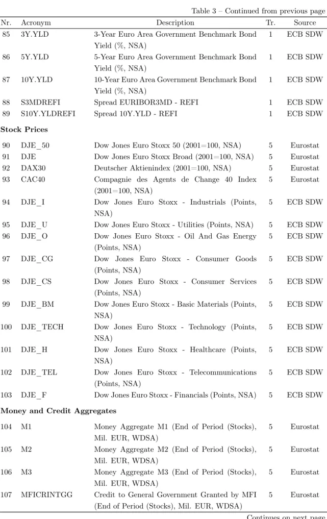
Figure 4: Impulse resp onses to a monetary tigh tening sho ck for the first alternativ e F A V AR ( Yt = GDP , HICP , in terest rate; sev en factors) ‐ 0. 40 ‐ 0. 20 0. 00 0. 20 0. 40 0 1 2 2 43 64 8 p.p. In te re st Ra te ‐ 0. 80 ‐ 0. 40 0. 00 0. 40 01 2 2 4 3 6 4 8 per c. GD P ‐ 0. 30 ‐ 0. 15 0. 00 0. 15 0 1 2 2 43 64 8 per c. HIC P ‐ 2. 00 ‐ 1. 00 0. 00 1. 00 01 2 2 4 3 6 4 8 per c. Indust ri al P roduct ion ‐ 3. 00 ‐ 1. 50 0. 00 1. 50 0 1 2 2 43 64 8 per c. Du rab le Co n s. ‐ 0. 40 ‐ 0. 20 0. 00 0. 20 0. 40 0 1 2 2 43 64 8 p.p. 6 ‐ mo n th Eu ri b o r ‐ 0. 15 0. 00 0. 15 0. 30 01 2 2 4 3 6 4 8 p.p. 10 ‐ ye ar Gover n . B o nds ‐ 0. 40 ‐ 0. 20 0. 00 0. 20 0. 40 0 1 2 2 43 64 8 per c. M3 ‐ 1. 50 ‐ 0. 75 0. 00 0. 75 1. 50 01 2 2 4 3 6 4 8 per c. Effe ct . Ex ch an ge Ra te ‐ 3. 00 ‐ 1. 50 0. 00 1. 50 0 1 2 2 43 64 8 per c. Ex ch an ge Ra te USD ‐ 6. 00 ‐ 3. 00 0. 00 3. 00 01 2 2 4 3 6 4 8 per c. Co mmo d it y Pr ic e Index ‐ 1. 50 ‐ 0. 75 0. 00 0. 75 0 1 2 2 43 64 8 per c. P roducer Pr ic e Index ‐ 1. 50 ‐ 0. 75 0. 00 0. 75 01 2 2 4 3 6 4 8 per c. HIC P ‐ En e rg y & U npr oc. Food ‐ 0. 10 0. 00 0. 10 0. 20 0 1 2 2 43 64 8 per c. HIC P ex cl udi ng En e rg y & U npr oc. Food ‐ 1. 50 ‐ 0. 75 0. 00 0. 75 01 2 2 4 3 6 4 8 p.p. Cap ac it y U tiliz at io n ‐ 0. 30 ‐ 0. 15 0. 00 0. 15 0 1 2 2 43 64 8 per c. C o nsum pt io n Ex pendi tu re ‐ 0. 30 ‐ 0. 15 0. 00 0. 15 01 2 2 4 3 6 4 8 per c. Em pl oy m e nt ‐ 0. 60 ‐ 0. 30 0. 00 0. 30 0 1 2 2 43 64 8 per c. Re ta il Tr ad e ‐ 0. 60 ‐ 0. 30 0. 00 0. 30 01 2 2 4 3 6 4 8 p.p. B u siness Cl im at e Indi ca to r ‐ 1. 00 ‐ 0. 50 0. 00 0. 50 01 2 2 4 3 6 4 8 per c. N o ndur ab le Co n s. Notes: P ercen tage deviations fr om the baseline for v ariables for whic h logarithms w ere tak en; p ercen tage p oin t deviations othe rwise. Num b er of mon ths after the monetary p olicy sho ck in the abscissa.
Figure 5: Impulse resp onses to a monetary tigh tening sho ck for the second alternativ e F A V AR ( Yt = GDP , HICP , in terest rate, exc hange rate; sev en factors) ‐ 0. 40 ‐ 0. 20 0. 00 0. 20 0. 40 0 1 2 2 43 64 8 p.p. In te re st Ra te ‐ 0. 80 ‐ 0. 40 0. 00 0. 40 01 2 2 4 3 6 4 8 per c. GD P ‐ 0. 40 ‐ 0. 20 0. 00 0. 20 0 1 2 2 43 64 8 per c. HIC P ‐ 2. 00 ‐ 1. 00 0. 00 1. 00 01 2 2 4 3 6 4 8 per c. Indust ri al P roduct ion ‐ 3. 00 ‐ 1. 50 0. 00 1. 50 0 1 2 2 43 64 8 per c. Du rab le Co n s. ‐ 0. 40 ‐ 0. 20 0. 00 0. 20 0. 40 0 1 2 2 43 64 8 p.p. 6 ‐ mo n th Eu ri b o r ‐ 0. 20 ‐ 0. 10 0. 00 0. 10 0. 20 01 2 2 4 3 6 4 8 p.p. 10 ‐ ye ar Gover n . B o nds ‐ 0. 60 ‐ 0. 30 0. 00 0. 30 0. 60 0 1 2 2 43 64 8 per c. M3 ‐ 2. 00 ‐ 1. 00 0. 00 1. 00 01 2 2 4 3 6 4 8 per c. Effe ct . Ex ch an ge Ra te ‐ 4. 00 ‐ 2. 00 0. 00 2. 00 0 1 2 2 43 64 8 per c. Ex ch an ge Ra te USD ‐ 6. 00 ‐ 3. 00 0. 00 3. 00 01 2 2 4 3 6 4 8 per c. Co mmo d it y Pr ic e Index ‐ 1. 50 ‐ 0. 75 0. 00 0. 75 0 1 2 2 43 64 8 per c. P roducer Pr ic e Index ‐ 2. 00 ‐ 1. 00 0. 00 1. 00 01 2 2 4 3 6 4 8 per c. HIC P ‐ En e rg y & U npr oc. Food ‐ 0. 20 ‐ 0. 10 0. 00 0. 10 0. 20 0 1 2 2 43 64 8 per c. HIC P ex cl udi ng En e rg y & U npr oc. Food ‐ 2. 00 ‐ 1. 00 0. 00 1. 00 01 2 2 4 3 6 4 8 p.p. Cap ac it y U tiliz at io n ‐ 0. 30 ‐ 0. 15 0. 00 0. 15 0 1 2 2 43 64 8 per c. C o nsum pt io n Ex pendi tu re ‐ 0. 40 ‐ 0. 20 0. 00 0. 20 01 2 2 4 3 6 4 8 per c. Em pl oy m e nt ‐ 0. 50 ‐ 0. 25 0. 00 0. 25 0. 50 0 1 2 2 43 64 8 per c. Re ta il Tr ad e ‐ 0. 75 ‐ 0. 50 ‐ 0. 25 0. 00 0. 25 01 2 2 4 3 6 4 8 p.p. B u siness Cl im at e Indi ca to r ‐ 1. 00 ‐ 0. 50 0. 00 0. 50 01 2 2 4 3 6 4 8 per c. N o ndur ab le Co n s. Notes: P ercen tage deviations fr om the baseline for v ariables for whic h logarithms w ere tak en; p ercen tage p oin t deviations othe rwise. Num b er of mon ths after the monetary p olicy sho ck in the abscissa.
The responses described above were, in general, also achieved by Bernanke et al. (2005) for the US and portray an intuitive description of the macroeconomy reaction to an increase in the official interest rates. Moreover, the extra information generated by the FAVAR approach brings to light some interesting results as regards the responses of the components of the HICP. In fact, it seems that the intuitive ne-gative response of inflation (total index) is strongly driven by the component energy and unprocessed food, which shows a big decrease after the policy shock. Howe-ver, when we look at the response of the HICP excluding energy and unprocessed food, we see that after an initial fall in the first five months following the shock, the prices start to increase (the magnitude of the response is not very relevant as the maximum impact is of 0.03 per cent in the first alternative FAVAR, but it never-theless constitutes a puzzle). One could find the strong response of the component energy and unprocessed food somewhat surprising, in particular taking into account that VAR models typically rest on the assumption that prices are sticky. However, as Boivin, Giannoni and Mihov (2009) draw attention to, recent evidence on the behaviour of disaggregated prices suggests that prices are much more volatile than conventionally assumed in studies based on aggregate data. The authors even prove that flexibility of disaggregate prices is perfectly compatible with stickiness of aggre-gate price indexes and that goods with little value added in final production, that is, energy-related good and fresh foods, display much more frequent price changes than the remaining components or price indexes. It must also be pointed out that, as expected, the response of the component energy and unprocessed food is very similar to the response of the producer price index, as shown in Figures 3 to 5.
Our analysis also reveals a counterintuitive response of the nominal effective exchange rate and the Euro/US dollar exchange rate (both defined in indirect quo-tation14). In fact, in all FAVAR specifications, a rise in the official interest rate is
associated with an initial depreciation of the euro, and this is against the economic rationale that a higher interest rate makes investment more attractive and therefore attracts capital inflows, causing the euro to appreciate. It is interesting to note that this against-theory result was also achieved by Laganà and Mountford (2005) for the United Kingdom and we believe that the justification they give also applies for the euro area: this result is probably caused by the euro area monetary authority reacting to changes in US (or other main trade partners) interest rates by changing the euro area official interest rate.15 Certainly, it could be argued that foreign policy 14This means that the cost of one unit of local currency (the euro) is given in units of foreign
currency. In the indirect quotation, an increase in the exchange rate represents an appreciation of the euro.
con-interest rates are part of our information set and therefore their movements should be captured by the factors. However, as Appendix B shows, none of the factors records a relevant correlation with foreign key interest rates. This may signal that not all dimensions of foreign monetary policy decisions are captured by our model, which is a natural result, taking into account that, as depicted in Appendix A, only 9 out of the 150 variables of the data set are “foreign variables”. Moreover, we believe that this result may be related to the fact that our sample encompasses the most acute phase of the world financial crisis (after September 2008) that was fuelled by the problems in the US subprime market. In fact, both the US Federal Reserve (FED) and the ECB started to cut their official interest rates after the be-ginning of the turbulence16 and during this period the euro appreciated against the
US dollar, which is in fact an intuitive response for the easing of the US monetary policy (i.e. as expected, the US dollar depreciates as a result of the decrease in US official interest rates). It must also be noticed that, in October 2008, the ECB intro-duced a number of changes to its monetary policy framework. In particular, until this date, the ECB used to conduct its refinancing operations through variable rate tenders in which the amount allotted was that corresponding to the amount bid at rates equal to or above the marginal rate. After October 2008, the ECB started to provide an unlimited amount of funds through its refinancing operations, which it began to conduct via fixed rate tenders at a rate equal to the policy rate and with full allotment. As the interbank money market practically stopped functioning during the financial crisis and as a consequence of the change in the Eurosystem’s operational framework, the ECB became the “preferred counterparty”, with credit institutions resorting heavily to its tenders to obtain the funds needed, and there-fore short-term liquidity conditions turned out to be very ample. Consequently, the EONIA rate fell considerably and stopped mimicking so well the behaviour of the ECB policy rate. An extension of our sample in the future, in particular encom-passing observations after the end of the crisis, may be needed to understand if it changes in a relevant way the impulse responses of the economic variables (and in particular if it annuls the counterintuitive results of exchange rates).
clusions, identifying monetary policy shocks in an open economy typically leads to substantial complications relative to the closed economy case, since the central bank’s actions not only res-pond to the state of the domestic economy but also to the state of foreign economies, including foreign monetary policy decisions. In this sense, a depreciation after a tightening shock may mean that this shock is “contaminated” by the systematic reaction of the monetary authority to foreign monetary policy and expected inflation.
16The FED started first, around September 2007, with the ECB postponing the use of a
3.2.3 Variance decomposition
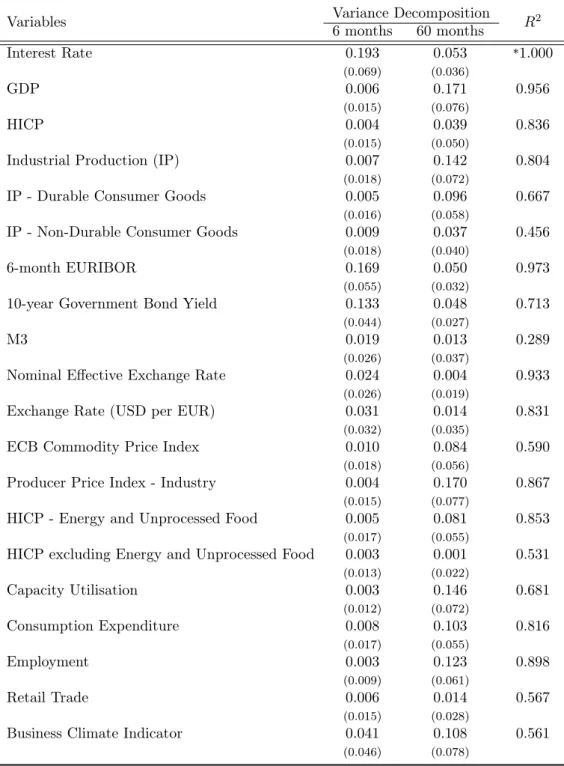
Forecast error variance decomposition is another exercise frequently performed when assessing the VAR results. It consists of determining the portion of the variance of the forecasting error of a variable, at anyt, that is attributable to a given shock and it follows immediately from the coefficients in the moving average representation of the VAR system and the variance of the policy shocks (Bernanke et al., 2005). It must be noticed that the FAVAR approach potentially provides a more accurate variance decomposition than the VAR approach because the relative importance of the policy shock is assessed only to the portion of the variable explained after removing the idiosyncratic component.
LetXbt+h|t be the optimal h-period ahead forecast of Xt+h on date t information
and Xt+h −Xbt+h|t the forecast error. The fraction of the variance of the forecast
error that is due to the monetary policy shock,εM P
t , may be expressed as:
V ar(Xt+h−Xbt+h|t|εM Pt )
V ar(Xt+h−Xbt+h|t)
(12) Table 2 reports the results for the same 20 macroeconomic variables analysed previously for our preferred FAVAR specification. The first two columns of Table 2 report the contribution of the monetary policy shock for the variance of the forecast error of each of the variables, at the 6-month horizon and the 60-month horizon, res-pectively. In order to access the goodness-of-fit properties of the estimated factors, the last column of Table 2 reports theR2 of the regression of each of the 20 variables on the common factorsCb(Ft, Yt), i.e. the fraction of each variable’s variance that is
explained by both Fbt and Yt. A high R2 indicates that the common factors nicely
summarise the information contained in the variable, whereas a lowR2 means that
the variable cannot be adequately explained by the common factors and implies that we must have less confidence in the impulse responses and forecast error variance decomposition computed.
There is an agreement in the literature that monetary policy shocks account for only a very modest percentage of the volatility of output and for even less of the movements in the price level (e.g. Christiano et al., 1999), so monetary policy affects the economy mostly through its systematic behaviour, rather than by surprising economic agents. In fact, looking at Table 2, we conclude that at the 6-month horizon, apart from interest rates, the contribution of the policy shock is lower than 5 per cent. In particular, less than 1 per cent of the variance of both GDP and HICP is accounted for by the shock. After 60 months, the monetary policy shock explains around 17 per cent and 14 per cent of the volatility of GDP and industrial
Table 2: Forecast error variance explained by the monetary policy shock
Variables Variance Decomposition R2
6 months 60 months Interest Rate 0.193 0.053 *1.000 (0.069) (0.036) GDP 0.006 0.171 0.956 (0.015) (0.076) HICP 0.004 0.039 0.836 (0.015) (0.050)
Industrial Production (IP) 0.007 0.142 0.804
(0.018) (0.072)
IP - Durable Consumer Goods 0.005 0.096 0.667
(0.016) (0.058)
IP - Non-Durable Consumer Goods 0.009 0.037 0.456
(0.018) (0.040)
6-month EURIBOR 0.169 0.050 0.973
(0.055) (0.032)
10-year Government Bond Yield 0.133 0.048 0.713
(0.044) (0.027)
M3 0.019 0.013 0.289
(0.026) (0.037)
Nominal Effective Exchange Rate 0.024 0.004 0.933
(0.026) (0.019)
Exchange Rate (USD per EUR) 0.031 0.014 0.831
(0.032) (0.035)
ECB Commodity Price Index 0.010 0.084 0.590
(0.018) (0.056)
Producer Price Index - Industry 0.004 0.170 0.867
(0.015) (0.077)
HICP - Energy and Unprocessed Food 0.005 0.081 0.853
(0.017) (0.055)
HICP excluding Energy and Unprocessed Food 0.003 0.001 0.531 (0.013) (0.022) Capacity Utilisation 0.003 0.146 0.681 (0.012) (0.072) Consumption Expenditure 0.008 0.103 0.816 (0.017) (0.055) Employment 0.003 0.123 0.898 (0.009) (0.061) Retail Trade 0.006 0.014 0.567 (0.015) (0.028)
Business Climate Indicator 0.041 0.108 0.561
(0.046) (0.078)
Notes: The figures in the column under “6 months” (“60 months”) report the fraction of the variance of the forecast error, at the 6(60)-month horizon, explained by the monetary policy shock. The last column reports the fraction of the variance of each variable explained by bothFbtandYt. Standard errors are shown in parenthesis. *This is by construction, since the interest rate is assumed to be the only variable observed.
production, respectively, and about 4 per cent of price volatility. In addition, the shock accounts for 10 per cent and 12 per cent of the variance of the prediction error of consumption expenditure and employment, respectively. Overall, these results surprisingly suggest a non-negligible role for the unsystematic component of monetary policy in affecting the dynamics of both real and nominal variables. Bernanke et al. (2005), in turn, find a more modest role for the policy innovations, since they conclude that apart from interest rates, the contribution of the monetary policy shock, at the 60-month horizon, ranges betwen 0 and 10 per cent.
On the other hand, an analysis of the last column of Table 2 reveals that the common component explains an important portion of the variance of some variables. Specifically, we obtain anR2 of 95.6 per cent, 80.4 per cent, 83.6 per cent, 89.8 per
cent, 93.3 per cent and 97.3 per cent for the GDP, industrial production, HICP, employment, nominal effective exchange rate and 6-month Euribor, respectively. However, there are also some variables for which the R2 is small, in particular the money aggregate M3 (28.9 per cent).
3.2.4 Robustness check
We have performed two types of robustness tests for the results of our preferred FAVAR specification. As a first step, the results were checked for robustness to changes in the number of factors (the number of factors was reduced to three, the number used in Bernanke et al. (2005), for the US). As a second step, we have treated the fed funds rate as an exogenous variable in order to work out if the responses change in a noteworthy way when we assume that there is no feedback from euro area variables to US monetary policy stance. The results for the the two robustness exercises are depicted in Appendix C and Appendix D.
In both cases, we still obtain considerable R2 for the majority of the variables,
and a lowR2 for the money aggregate. In the first robustness check, the shape and
magnitude of the responses does not change in a very significant way, although the return to baseline is more slow for most of the variables. However, the exception worth mentioning is the behaviour of the HICP, as when we reduce the number of factors, the price puzzle starts to be visible. This is not very surprising if we take into account that according to the tentative interpretation of the factors performed in Appendix B both the second and the fourth latent factors seem to capture cyclical variations in inflation and we are not considering the latter in this exercise. In the second robustness test, although the magnitude of the responses does not change in a very relevant way, the effects are even more long-lasting than in the first test.