Global Production with Export Platforms
Felix Tintelnot
∗University of Chicago and NBER
November 21, 2015
Abstract
Most international commerce is carried out by multinational firms, which use their foreign affiliates both to serve the market of the host country and to export to other markets outside the host country. In this paper, I examine the determinants of multinational firms’ location and production decisions and the welfare implications of multinational production. The few existing quantitative general equilibrium models that incorporate multinational firms achieve tractability by assuming away export platforms – i.e. they do not allow foreign affiliates of multinationals to export – or by ignoring fixed costs associated with foreign investment. I develop a quantifiable multi-country general equilibrium model, which tractably handles multinational firms that engage in export platform sales and that face fixed costs of foreign investment. I first estimate the model using German firm-level data to uncover the size and nature of costs of multinational enterprise and show that the fixed costs of foreign investment are large. Second, I calibrate the model to data on trade and multinational production for twelve European and North American countries. Counterfactual analysis reveals that multinationals play an important role in transmitting technological improvements to foreign countries and that the pending Canada-EU trade and investment agreement could divert a sizable fraction of the production of EU multinationals from the US to Canada.
JEL Codes: F12, F23, L23
Keywords: multinational enterprise, production location decisions, export platform, constrained maximum likelihood estimation
∗I am grateful to my advisors Jonathan Eaton and Stephen Yeaple for their guidance, encouragement, and support. I am also
grateful to Andr´es Rodr´ıguez-Clare and Paul Grieco for encouragement and various discussions on the topic. I wish to thank the editor, Elhanan Helpman, and three anonymous referees for their comments and suggestions. I thank Pol Antras, Costas Arkolakis, Kerem Cosar, Anca Cristea, Teresa Fort, Anna Gumpert, Christian Gourieroux, Oleg Itskhoki, David Jinkins, Corinne Jones, Sung Jae Jun, Konstantin Kucheryavyy, Matthias Lux, Kalina Manova, Eduardo Morales, Andreas Moxnes, Joris Pinkse, Natalia Ramondo and seminar participants at Arizona State University, Boston University, University of Chicago, University of British Columbia, MIT, University of Michigan, NBER Summer Institute, Pennsylvania State University, Stanford University, University of Wisconsin, and Yale University for helpful comments and suggestions. I thank the German Bundesbank for the hospitality and access to its Microdatabase Direct investment (MiDi). This paper is part of my PhD dissertation at Penn State. I continued working on this project while visiting the International Economics Section at Princeton University, whom I thank for their hospitality. Ken Kikkawa and Zhida Gui provided outstanding research assistance. This work was completed in part with resources provided by the University of Chicago Research Computing Center. All errors are my own. Correspondence:[email protected].
1
Introduction
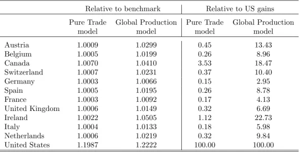
Multinational firms account for a large share of global output and employment.1 In structuring their global operations, these firms confront various costs of multinational production and trade. For instance, whether a firm should pursue a strategy of maintaining many plants to avoid shipping costs or a strategy of consolidating production in a few locations turns on the size of the fixed costs of establishing foreign plants relative to the costs of shipping goods. Further, given a set of production locations, the choice of which product to produce where depends on the interaction of comparative advantage and the cost of shipping goods. In the data, firms tend to concentrate their production in only a few locations, which is intuitive under increasing returns at the plant level, and to use export platform sales in order to serve markets outside the host country. For US multinationals’ affiliates in Europe, Figure 1 documents the proportion of output exported to other countries from the host country. Across all countries (including countries outside Europe), export platform sales account for an average of 43 percent of multinationals’ foreign output, a share that is systematically higher for smaller countries.
In this paper, I develop a framework that is designed to answer several key questions. First, what are the costs associated with multinational production? How important are the fixed costs of establishing foreign operations relative to possible efficiency losses due to remote management? Second, how does the process of globalization, measured as a fall in these costs, affect the structure of global production? Will globalization result in firms’ consolidating production in a few favored locations, or will firms expand their global production networks? Third, how does allowing for multinational production affect our understanding of the welfare effects in a general equilibrium trade model?
Export platform sales, together with the presence of fixed cost of establishing foreign plants, imply a hard permutation problem for deciding on how to structure a firm’s global operations. A firm simultaneously needs to decide the set of countries in which to establish a production plant, which markets to serve from each plant, and how much to sell to each market. Perhaps for this reason, the literature on multinational firms in multi-country settings has made extreme assumptions. Existing work either does not allow for export platform sales or ignores the fixed costs of establishing foreign plants. The key idea for tractability in the framework presented in this paper is to consider a firm as consisting of a continuum of products and to treat a firm’s product-location-specific productivities as random variables, similarly to how Eaton and Kortum (2002) treat a country’s productivities. By allowing each firm to produce a continuum of products, I smooth out the firm’s 1A multinational firm is a company with enterprises in more than one country. I define its home country as the country in
which the parent company of the enterprises is registered. Usually, this coincides with the country of the multinational firm’s headquarters. According to Bernard, Jensen, and Schott (2009), in the year 2000 multinational firms accounted for nearly 80 percent of US imports and exports, and employed 18 percent of the entire US civilian workforce. Publicly available BEA data shows that, in the manufacturing sector, the sales by US MNEs’ majority-owned foreign affiliates are more than twice as large as aggregate US exports.
Figure 1: Export platform shares for US multinationals in Europe
Notes: This figure displays the share of output that is exported to countries outside the host country by US multinationals’ majority-owned foreign affiliates in the manufacturing sector. For the European countries displayed in the figure, typically only about 5 percent of the output is sold back to the US. An exception is Ireland, for which 17 percent of the output is sold to the US. Across all countries (including countries outside Europe), US-owned foreign affiliates in the manufacturing sector sell 43 percent of their output to countries outside the host country – 13 percent of the output is sold to the US and 30 percent to other foreign countries. The statistics are for the year 2004. Source: BEA.
response to changes in aggregate variables and obtain intuitive, closed-form expressions for the output at each of the firm’s plants. A firm’s output is a function of the locations of its plants, the productivity of each plant, the input costs in the plants’ host countries, and the market potential of the plants’ host countries. Furthermore, the model delivers a probability with which a firm chooses a set of plants, as the fixed cost to establish a plant in a foreign country is stochastic and firm-country-specific.
With this framework, I conduct a two-tiered empirical analysis. Using German firm-level data on output at the parent and affiliate levels, I estimate both the variable production costs in foreign countries as well as the distribution of fixed costs to establish a foreign plant. I find that German multinational firms face between 5 percent (Austria) and 35 percent (United States) larger variable production costs abroad than at home and face substantial fixed costs of establishing foreign affiliates. I also document that multinational firms tend to produce
a large share of their output domestically and that this pattern is robust across size cohorts and industries. In the second tier of my empirical inquiry, I focus on general equilibrium welfare analysis. I calibrate the general equilibrium outcomes of the model to match data on bilateral trade flows, bilateral shares of foreign production, and the country-specific production cost estimates from German multinational firms. The cost estimates of German multinationals enable me to include both variable foreign production frictions and fixed costs in the analysis that otherwise includes only aggregate data. I solve for the endogenous relative wages and price indices in every country. With the calibrated model, I explore how globalization changes the structure of global production. For example, currently, Canada and the EU are in the ratification process of a trade and investment agreement: CETA. If one supposes that the agreement is signed and yields a 20 percent reduction of variable and fixed production costs between the signatories, then – according to my calibrated model – EU multinationals would divert around five percent of their production from the US to Canada. These findings hinge on the possibility of export platform sales from Canada to the US. Without this possibility, the location and output decisions of European firms are independent between Canada and the United States. Instead, I find that a Canada-EU trade and investment agreement could induce a strong third-party effect on the United States.
Furthermore, I demonstrate that a more complete model of multinational production and trade can revise answers to classic questions in the trade literature. Specifically, I investigate how technology shocks in one country affect production and welfare outcomes in all countries, a question often studied in trade models without multinational production. Multinational production provides an additional channel through which technology can flow across countries. Suppose all US firms improve their technology by 20 percent. I find that the welfare gains in foreign countries from such a technology improvement are an order of magnitude larger when multinational production is taken into account. The magnitude of the gains in foreign countries depends crucially on the cost of foreign production, which I carefully estimate in this paper. In models without multinational production, the cost of foreign production is infinite by assumption.
The model presented in this paper combines elements of Helpman, Melitz, and Yeaple (2004) and Eaton and Kortum (2002). As in Helpman, Melitz, and Yeaple (2004), firms produce differentiated goods and can establish foreign plants at the expense of fixed costs.2 I extend their framework by incorporating export-platform sales and multi-product firms. As in Eaton and Kortum (2002), countries differ in their comparative advantage in production. In my model, however, each product can be produced only by a single firm, which can also produce in foreign countries, while Eaton and Kortum (2002) instead assume that each firm operates only domestically and that firms from different countries can produce the same product. If multinational production is prohibitively costly, my model collapses with respect to its aggregate predictions to Anderson and 2Helpman, Melitz, and Yeaple (2004) combine key elements that appeared in Melitz (2003) and Horstmann and Markusen
van Wincoop (2003), and the product-location-specific productivity draws have no impact.
I also build on and contribute to a vibrant area of ongoing research that centers on the gains from multinational production and trade. Ramondo and Rodriguez-Clare (2013) develop a quantitative framework for multinational production and trade. Their paper extends the Ricardian trade model by Eaton and Kortum (2002) insofar as it allows the technologies that originated in a country to be used for production abroad. Their paper provides a tractable framework to analyze trade and multinational production in a Ricardian world. They investigate the gains from trade, multinational production, and openness and find the gains from trade can be twice as large if multinational production is taken into account. Arkolakis, Ramondo, Rodriguez-Clare, and Yeaple (2013) take the insights of Ramondo and Rodriguez-Clare (2013) to a parameterized version of the Melitz model. Their framework endogenizes firms’ initial entry decisions in a setting featuring comparative advantage and increasing returns to scale, allowing them to analyze the allocation of innovation and production across countries. They show that endogenizing entry is important, as shocks that induce a relocation of innovation abroad can reduce a country’s welfare. Neither of these papers allows for fixed costs of foreign production, and both have difficulty generating export platform sales that are of the right order of magnitude.3 While my model fits the export platform sales of US multinationals well (without having aimed to fit those in the calibration), a restricted version of my model without fixed costs generates lower export platform sales. Both fixed and variable costs discourage foreign production, but it is the fixed costs that induce firms to concentrate their production in a few locations.4
My findings that multinational firms face significantly larger variable production costs abroad and significant fixed costs of establishing foreign plants are in line with the findings of Irarrazabal, Moxnes, and Opromolla (2009). They use data from Norwegian firms and develop a structural model that extends Helpman, Melitz, and Yeaple (2004) by incorporating firm trade, and they find that a very large share of intra-firm trade is necessary to rationalize the observed output data.5 Their paper ignores export platform sales, however, which makes the set of production strategies among which a firm can choose much smaller. Without 3In Ramondo and Rodriguez-Clare (2013), only when the productivity draws for ideas that originated in one country are
uncor-related across countries can the calibrated model come close to matching the data on export platform sales for US multinationals. The calibrated model in Arkolakis, Ramondo, Rodriguez-Clare, and Yeaple (2013) generates much lower export platform sales for US firms than in the data.
4Fixed costs and export platforms have been analyzed together only in very restrictive settings. Neary (2002) shows in a
theoretical analysis that with export platform sales and fixed costs of establishing foreign plants, the European single-market policy increases foreign direct investment into the EU from outside countries. Ekholm, Forslid, and Markusen (2007) develop a three-country model that incorporates both fixed costs and export platform sales. Other three-country models with fixed costs and complex relationships between domestic and foreign plants have been developed by Yeaple (2003) and Grossman, Helpman, and Szeidl (2006). These last two papers allow for more complex integration strategies of firms than my model. However, it is impractical to apply their model to the data of many countries. Head and Mayer (2004) apply a model with multiple countries, fixed costs, and sales to surrounding markets to data on Japanese affiliates under the restriction that each firm can only have a single production location. The interdependence between firms’ location and production decisions has been reflected in empirical work by Baltagi, Egger, and Pfaffermayr (2008) and Blonigen, Davies, Waddell, and Naughton (2007), who apply spatial econometric methods to data on bilateral FDI and multinational firms’ sales and point out significant third-country effects in their estimation results.
5Instead of assuming intra-firm trade, I allow the production efficiency of foreign affiliates to differ from the production efficiency
the possibility of export platform sales, the decision of a European firm to set up an affiliate in the United States is independent of the decision to set up an affiliate in Canada, for example.6
Since in my model firms choose a set of production locations instead of making independent decisions about whether to establish a plant for each country, this paper also joins a literature that studies large discrete choice problems at the firm level.7 Morales, Sheu, and Zahler (2015) estimate a dynamic trade model in which the costs of serving a foreign market depend on the set of foreign markets the firm had served in the past. This creates an interdependency between the destination markets. Interdependent location choices within the firm also arise in Holmes (2011), who estimates the determinants of the expansion of Walmart stores within the United States. Both papers use moment inequalities to conduct their estimations. By contrast, the parameters in my model are point-identified, enabling me to conduct general equilibrium and counterfactual analysis.
The rest of the paper proceeds as follows. Section 2 outlines the model. Section 3 estimates country-specific fixed and variable production costs for German multinational firms via constrained maximum likelihood. Section 4 calibrates the general equilibrium, and Section 5 conducts the counterfactual exercises described above. Section 6 concludes.
2
A model of global production with export platforms
I develop a model that explains in which countries firms locate their plants, how much they produce in each country, and how much they ship from one country to another. Geography is reflected in three kinds of barriers between countries: variable iceberg trade costs, variable efficiency losses in foreign production, and fixed costs to establish foreign plants. Countries differ in endowments of labor and the mass and distribution of firms. While the technology of local firms is part of the endowments, the set of firms that produce in a country is determined endogenously. I assume a market structure characterized by monopolistic competition.
The model describes a novel view of the firm in the global economy. In a nutshell, I put the structure developed by Eaton and Kortum (2002) inside a single firm. This involves thinking of the firm as consisting of a continuum of products, with product-location-specific productivity shocks. However, a firm can produce in a country only after paying a fixed cost of establishing production operations in that country, which are also firm-country-specific. The advantage of this novel view of the firm is particularly visible when it comes to empirical applications, which are described in more detail later on. However, it will be useful to give a quick preview here. Firm-level data on multinational firms commonly comes with information on the set of countries 6Existing work on structural estimation with data on multinational firms is sparse. Exceptions are Feinberg and Keane (2006)
who structurally estimate US multinationals’ decisions to invest and produce in Canada, and Rodrigue (2014) who structurally estimates a model of trade and FDI with data on Indonesian manufacturing plants.
7The decision as to where to establish facilities and which market to serve from which facility is known as the ‘Facility Location
Problem’ in operations research. See Klose and Drexl (2005) for a survey of the literature on the ‘Facility Location Problem,’ which is primarily concerned with developing solution algorithms to the single firm’s problem.
in which the firm produces and information on total output of the firm in each location conditional on the set of production locations. The model delivers smooth and intuitive expressions for these economic terms while they would be intractable step functions for a single product firm. In particular, I derive profit and sales functions for a firm when selecting a particular set of production locations that are smooth in all parameters (trade costs, fixed costs, etc.) and a probability with which a firm selects a particular set of production locations. These expressions are imbedded in a general equilibrium framework, and my model contains the standard gravity trade model without multinational production as a special case.
I start with the description of demand and then turn to the problem of the firm.
2.1
Demand
I assume standard CES preferences, with the distinction that here each firm has a continuum of products instead of a single product.8 A good is indexed by a firm ω and a variety υ. I assume a measure 1 of varieties per firm and a fixed measure of firms.9 If the representative consumer of countryj consumesq
j(ω, υ) units of each
variety υof each firmω∈Ω, she gets the following utility:
Uj≡ Z Ω 1 Z 0 qj(ω, υ)(σ−1)/σdυdω σ/(σ−1) . (1)
The elasticity of substitutionσ >1 is identical between varieties inside and outside the firm. Assuming the same elasticity of substitution between varieties within the firm and between varieties from different firms simplifies the pricing decision by the firm. Consumers maximize their utility by choosing their consumption of goods subject to their budget constraint. I denote the aggregate income in countryjbyYj.Utility maximization
implies that the quantity demanded in countryj of variety υ supplied by firmω at pricepj(ω, υ) is
qj(ω, υ) =pj(ω, υ)−σ
Yj
Pj1−σ, (2)
wherePj is the ideal price index in countryj:
Pj≡ Z Ωj pj(ω)(1−σ)dω 1/(1−σ) , (3)
8A modification of my model in which each firm produces a single final good – which is a CES aggregate of a continuum of
intermediates – and assuming that the firm sets intra-firm prices with a constant mark-up over marginal cost, yields isomorphic firm-level and aggregate predictions. Since I can determine the optimal pricing rule in the final goods interpretation endogenously, I focus on the continuum of final goods interpretation in the text below.
9Antr`as, Fort, and Tintelnot (2014), who build on the framework presented in this paper, show how to endogenize the number
of varieties per firm and derive the prediction that more productive firms have more varieties. Additional data would be necessary to identify the cost of adding varieties.
which is simply the standard CES price index over the firm-level price indices. The price index of firm ω to countryj is pj(ω)≡ 1 Z 0 pj(ω, υ)1−σdυ 1/(1−σ) , (4)
and the expenditure on goods produced by firmω in countryj is
sj(ω) =pj(ω)1−σ
Yj
Pj1−σ. (5)
Next, I proceed to describe the problem of a single firm.
2.2
The firm’s problem
Each firm behaves like a monopolist and faces a CES demand function for each of its products. Every firm is infinitesimal and takes aggregate price indices, income, and wages as given. The problem of the firm consists of two stages: first, the firm selects the set of countries in which to establish a plant in order to maximize expected profits; it then learns about the exact quality of each plant and decides which market to serve from which location for each product.10 For simplicity, I assume there are no fixed costs associated with exporting and, consequently, every product is sold to every market.11
A firm is characterized by its country of origin,i, its core productivity parameter,φ, a vector of fixed cost levels in every country,η, and a vector of location-specific productivity shifters, . All these variables are firm-specific. There areN countries.
2.2.1 Production decisions after the plants are selected
Denote by Z the set of locations the firm has selected for production plants. I assume that a firm always has a plant in its home country. In those countries in which the firm has established a plant, the firm draws a location-specific productivity for each of its products from a Fr´echet distribution.12 Letν
jbe a random variable
that denotes the productivity level in countryj for a particular product. The cumulative distribution function 10Without firm-plant-specific shocks the model would have zero likelihood as the ratio of output of two firms with the same set
of production location would be identical across countries, which is not the case in the data. The timing assumption - the firm learns about the quality of each plant after the set of production locations is selected - simplifies the analysis of firm-level data for reasons that I will discuss in Section 3.
11Fixed costs of exporting (at the firm level) could be incorporated, similarly to Eaton, Kortum, and Kramarz (2011) and
Arkolakis, Ramondo, Rodriguez-Clare, and Yeaple (2013), but they are omitted for simplicity and would require additional data to be identified. After laying out the firm’s problem in the following pages, I describe below in footnote 16 how fixed costs of exporting could be incorporated specifically and perform sensitivity analysis to the empirical results in Section 3.4.
of a product’s productivity in country j is: Pr(νj ≤x) = exp −(φj) θ (γijx)− θ .
The product of the core productivity level,φ, and the plant-specific productivity shifter,j, determines
the level of the productivity draws in the plant in country j. Larger values of φj imply better productivity
distributions.13 The dispersion of the productivity draws is decreasing inθ. All firms from countryimay have lower productivity in countryl, which is captured by an iceberg loss in production, γil. These losses may for
example occur because of higher costs due to communication challenges, information frictions, or shipments of intermediate products. For technical reasons I imposeθ >max(σ−1,1).
At each location, the firm transforms units of labor into goods at a constant marginal cost inversely proportional to productivity. The wage in country j is denoted bywj. Trade costs to ship goods from country
l tomare of the iceberg type and are denoted byτlm. Given these assumptions about production and shipping
technology, it is easy to derive that the costs to serve marketmfrom countryl∈Z are distributed as
Pr w lτlm νl ≤c = 1−exp − γ ilwlτlm φl −θ cθ ! .
Having its production plants in place, the firm selects, for each product and market, the production location that can supply that market at the minimum cost. Using the known properties of the Fr´echet dis-tribution, one can derive that the product-level costs with which the firm will serve marketm are distributed according to Gm(c|i, φ, Z, ) = 1−exp − X k∈Z γ ikwkτkm φk −θ cθ ! . (6)
With CES preferences and monopolistic competition, the firm charges a constant mark-up, σ−σ1, for each good over the unit cost of delivering the good to each market. Using the optimal pricing rule, and the distribution of product-level costs, (6), we can write the firm-level price index – defined in (4) – which aggregates the product-level prices that the firm (i, φ, Z, ) charges in marketm, as
pm(i, φ, Z, ) =κ 1 1−σφ−1 X k∈Z (γikwkτkm)−θθk !−1/θ , (7) whereκ= Γ θ+1θ−σ σ σ−1 1−σ
is a constant.14 The total sales of firm (i, φ, Z, ) in marketmare
13The reader familiar with Eaton and Kortum (2002) may recognize the similarity between the country-specific parameterT
jin
their paper and the firm-country-specific parameterφjin this paper.
14This step is analogous to the calculation of theoverallprice index in Eaton and Kortum (2002) and uses the moment generating
sm(i, φ, Z, ) =pm(i, φ, Z, )1−σ
Ym
Pm1−σ
. (8)
The expressions for the firm’s price index, (7), and total sales, (8), in marketmhave intuitive properties: the sales rise in the core productivity level of the firm; furthermore, the firm benefits particularly from having a plant in a countrykin which the variable costs to supply marketmare low (lowγikwkτkm), and in which the
firm has a large plant-wide productivity shifter (largek).
Due to constant returns to scale in the variable production costs, the firm will simply choose for each variety the location with the lowest unit cost to serve a market. We can write the share of products for which the plant in countryl is selected to serve countrymas
µlm(i, φ, Z, ) = Pr argmin j∈Z γijwjτjm νj =l = (γilwlτlm)−θθl P k∈Z (γikwkτkm)−θθk ifl∈Z 0 otherwise. (9)
The share of goods that a firm ships from countryl to country mis large if the plant in countryl has low costs to serve market m relative to the firm’s other plants. If the firm has a plant in country l (l ∈ Z), the product-level cost at which a firm actually supplies market m from location l also has the distribution Gm(c|i, φ, Z, ). Consequently,µlm(i, φ, Z, ) equals not only the share of products that a firm with location set
Z ships from locationlto marketm, but also the corresponding value share. Therefore, the sales from location l∈Z to marketm for such a firm are
slm(i, φ, Z, ) = Ym Pm1−σ | {z } market demand inm × (γilwlτlm) −θ θl P k∈Z (γikwkτkm)−θθk | {z }
% products sourced froml
× κ X
k∈Z
(γikwkτkm)−θ(φk)θ
!σ−θ1
| {z }
price index of firm inmto the power of 1−σ
. (10)
My model implies a gravity equation for the firm-level sales. As in Melitz (2003), a firm’s sales from country l to country m are rising in the firm’s core productivity level, φ, and the market demand of the destination country, Ym
Pm1−σ
, and decreasing in the trade barriers between the countries, τlm, and production
wages,wl. Interestingly, here the production barriers for firms from countryito produce in countryl,γil, also
product are alternative source countries in serving the destination country,m.15 16
The total revenue of the plant in country l ∈ Z arises from sales to all countries from this plant and can be written as rl(i, φ, Z, ) =κφσ−1 X m Ym Pm1−σ (γilwlτlm) −θ θ l P k∈Z (γikwkτkm)− θ θ k (θ+1θ−σ) . (11)
I summarize the relationship between a firm’s plants in Proposition 1, whose proof is in the appendix. Proposition 1. The firm-level sales to each market increase as additional production locations are added to the set of existing locations. However, there is a cannibalization effect across production locations. That is, a firm that adds a production location decreases the sales from the other locations.
The revenue expression in (11) provides a generalization of the market potential concept considered by Redding and Venables (2004), Head and Mayer (2004), and Hanson (2005). As in their papers, a plant’s market potential depends on the local and surrounding countries’ market demand weighted by the trade costs. In addition, here the set of other plants the firm owns and the other plants’ proximity to the markets matter for the sales volume. The market potential collapses to their measure for firms with plants in only a single country. Interestingly, the cannibalization effect across production locations becomes weaker as the Fr´echet parameter of the productivity draws, θ, falls. In the limit, as θ → σ−1, the dispersion of the draws across production locations is so large that all of the plants obtain their revenues from distinct products, and the cannibalization effect disappears. To see this formally, note that the denominator in (11) approaches unity if θ → σ−1. Therefore, my model nests another, simpler model of global production in which each plant of a firm produces a distinct product.
Next, I proceed to examine the optimal choice of the set of locations,Z.
2.2.2 Choice of production locations
There are various motivations for setting up foreign plants: a foreign plant yields proximity to the local and surrounding markets, may have lower factor costs, and, finally, has a comparative advantage in the production
15In Melitz (2003), firms produce only in their country of origin, i.e.γ
il=∞ifi6=l. In this case, (10) simplifies toslm(i, φ, Z, ) =
0 ifi6=landslm(i, φ, Z, ) =κ Ym Pm1−σ wlτlm φl 1−σ ifi=l.
16One may want to consider a richer version of the model in which firms face a fixed cost of market access,ι
mwi. Consequently, a
firm would serve marketmonly if 1σsm(i, φ, Z, )≥ιmwi. LetsMAClm (i, φ, Z, ) denote the firm-level sales from locationlto market
mimplied by the model augmented with a fixed market access cost. Then,
sMAC lm (i, φ, Z, ) = ( slm(i, φ, Z, ) 0 if σ1sm(i, φ, Z, )≥ιmwi otherwise .
Importantly, such fixed costs of market access are independent of the set of production locations used to serve the particular market. If the fixed costs of market access were a function of the set production locations used to serve a market, a firm would no longer always choose for each product the minimum cost location to serve a particular market, and the model would loose tractability.
of some of the firm’s products. On the other hand, the firm incurs a fixed cost for establishing a foreign plant, which motivates the firm to concentrate its production in as few locations as possible. The firm selects a set of production locations based on its core productivity level,φ, its fixed cost draws,η, and its country of origin, i. As it is assumed that a firm always has a plant in its home country, in total, there are 2N−1feasible combinations of locations. I denote the set that contains all sets of locations for a firm from country i byZi. Fixed costs
have to be paid in units of labor from the host country. If the firm chooses the set of locationsZ∈ Zi, the firm
incurs fixed costs equal toP
l∈Zηlwl.
The firm chooses the set of locations that maximizes its expected profits. The expected variable profits from Z are simply the sum of the expected sales to all markets multiplied by the proportion of sales that represents variable profits:
E(π(i, φ, Z, )) = 1 σ X m E(sm(i, φ, Z, )). (12)
The total expected profits of set Z are the expected variable profits minus the fixed cost payments associated with the locations contained in the set. I assume that no fixed costs have to be paid for the domestic plant (or that they have been paid in the firm’s entry stage that I do not include in this model). The expected total profits from choosing a set of locationsZ are thus:
E(Π(i, φ, Z, , η)) =E(π(i, φ, Z, ))−
X
k∈Z,k6=i
ηkwk. (13)
I write the set of locations that maximizes the expected profits as
Z(i, φ, η)∈arg max
Z∈ZiE(Π(i, φ, Z, , η)). (14)
While, in general, multiple sets of locations could be optimal for the firm, as long as the fixed cost vectorηis drawn from a continuous distribution (where the draws are independent across countries), the set of fixed cost shock vectors for which the firm is indifferent across two or more location sets has measure zero.
In the following subsection, I turn to describing the endowments of each country, the aggregation of the firms’ choices, and the global production equilibrium.
2.3
Equilibrium
Countryjis endowed with a populationLj and a continuum of heterogeneous firms of massMj. I assume that
byFi(η) that can differ by the country of origin,i, is continuous, and has the positive orthant as its support.17 The core productivity level,φ, and the vector of location-specific productivity shifters,, can be realizations of arbitrary (potentially degenerate) distributions, which are denoted byG(φ) andH(), respectively.
Now I proceed to aggregate over the individual firms’ choices to establish expressions that I use in the definition of the global production equilibrium below. The share of firms from countryiwith core productivity φthat choose location setZ is
ρi,φZ = Z
η
1[Z(i, φ, η) =Z]dFi(η). (15)
This formulation is used in the derivation of the total sales of firms that originated in country ifrom country l to country m, Xilm. We can simply integrate over the core productivity levels of the firms from
countryi, and write their sales as the weighted sum of the sales a firm would make from countryl to country m conditional on a location set, where the weights are the probabilities with which the firm actually chooses this location set:
Xilm=Mi Z φ X Z0∈Zi ρi,φZ0E(slm(i, φ, Z0, ))dG(φ). (16)
Aggregate trade flows from country l to m are then simply the sum of the termXilm across all countries of
origin:
Xlm=
X
i
Xilm. (17)
Following (3), the consumer price index in market m, Pm, consists of the firm-level price indices for
marketm of firms from all countries. Again, the expression is the integral over the core productivity levels of the firms and a weighted sum of the firms’ price indices conditional on their location choice:
Pm= X i Mi Z φ X Z0∈Zi ρi,φZ0E(pm(i, φ, Z0, )1−σ)dG(φ) 1/(1−σ) . (18)
In order to establish the labor market clearing condition for country k, I define the set of feasible location sets for firms from country i that include a location in country k as ∆i
k ={Z ∈ Zi | k∈ Z}. Total
labor income in country k is equal to the sum of the wages paid in production in countryk by firms from all countries and of the wages paid in plant construction by foreign companies:
wkLk= σ−1 σ X m Xkm+ X i6=k Mi Z φ Z η X Z∈∆i k 1[Z(i, φ, η) =Z]ηkwkdFi(η)dG(φ). (19)
17For instance, the fixed costs to produce domestically are assumed to be zero, which generates differences among the fixed cost
I assume that a representative household owns the domestic firms.18 The aggregate income in country iis then the sum of the labor payments and the profits by firms that originated in countryi:
Yi=wiLi+Mi Z φ Z η X Z∈Zi 1[Z(i, φ, η) =Z]E(Π(i, φ, Z, , η)dFi(η)dG(φ). (20)
Now that I have defined the expressions above, I can define the global production equilibrium.
Definition 1. Given τij, γij, Fi(η), G(φ), H(), Mi,Zi,∀i, j = 1, ..., N, aglobal production equilibrium is a set of wages, wi, price indices, Pi, incomes, Yi, allocations for the representative consumer, q(ω, υ), prices,
pm(i, φ, Z, ), and location choices,Z(i, φ, η), for the firm, such that
(i) equation (2) is the solution of the consumer’s optimization problem. (ii) pm(i, φ, Z, )andZ(i, φ, η)solve the firm’s profit maximization problem.
(iii) Pi satisfies equation (18).
(iv) The labor market clearing condition, (19), holds. (v) Yi satisfies equation (20).
Since the model is static, utility maximization implies current account balance. However, it is possible that a country runs a trade deficit, which is financed by the profits that this country’s multinational firms generate abroad.
In the following section I apply this model to data from German multinational firms to identify the determinants of firms’ production and location choices. In this first tier of my empirical analysis, I take wages, aggregate income, and price indices in countries as given.
3
Estimation of fixed and variable production costs
In the first tier of the empirical analysis, I use firm-level data on German multinational firms in the manufacturing sector to measure the fixed and variable production costs by German firms in various countries. When using only aggregate data, previous work by Ramondo and Rodriguez-Clare (2013) estimated very large differences between firms’ productivities at home and outside the country in which a firm’s headquarters is located. Their estimates imply that the same product can be produced abroad with costs on average about 3.5 times as high as at home. The idea here is that using firm-level data and a within-firm comparison of production activities 18This seems to be a reasonable assumption: according to Cummings, Manyika, Mendonca, Greenberg, Aronowitz, Chopra,
Elkin, Ramaswamy, Soni, and Watson (2010), in 2007, US residents held 86 percent of the total market value of all US companies’ equities either directly as individual investors or indirectly through pension funds and retirement and insurance accounts.
across countries to measure these frictions likely leads to estimates that are more plausible. Also, the micro data enables me to measure both variable and fixed barriers to foreign production, which would be impossible with aggregate data on multinational production (MP) only.
This Section proceeds as follows. Subsection 3.1 describes the data sources, and Subsection 3.2 doc-uments that German firms tend to concentrate their production in only a few countries, and – conditional on being active in a foreign country – produce less in that foreign country than the relative size of the foreign econ-omy (measured in GDP or gross production) would suggest if multinationals were free to move their production abroad without any frictions. Subsection 3.3 describes the estimation of fixed and variable costs of foreign production with constrained maximum likelihood, whose parameter estimates are presented in Subsection 3.4. Finally, Subsection 3.5 conducts a counterfactual analysis to document the quantitative importance of each of these barriers.
3.1
Data description
My analysis in this section is based on firm-level data on German multinational firms in the manufacturing sector. By law, German resident investors are required to report on the activities of foreign affiliates if the affiliate has a balance sheet total above 3 million Euro and the investor has a share of voting rights of 10 percent or more. The information about the foreign affiliates is contained in the Microdatabase Direct Investment (MiDi) which is maintained by the German Bundesbank.19 I use data for the year 2005 for affiliates that belong to the manufacturing sector and that are majority-owned by a parent firm in the manufacturing sector. I focus on German multinationals’ activities in twelve Western European and North American countries.20 I take the set of countries in which a multinational owns an affiliate (including the home country) as the corresponding data analogue to the set of production plants in the model. I observe the total sales for each affiliate as well as the total sales for the parent company.21 In addition, I use data on all domestic, non-foreign-owned German manufacturing firms from the Amadeus database. I add these firms to the empricial analysis, since producing only domestic is an endogenous choice in the model, and ignoring such outcomes would lead to biased estimates in the likelihood estimation below.22 Aside from firm-level data, I use several variables calculated from aggregate data. I use data on gross production and bilateral trade flows from the OECD STAN database to calculate 19Other research uses of the database include Muendler and Becker (2010), who study the margins of multinational labor
substitution for multinational firms, and Buch, Kleinert, Lipponer, and Toubal (2005), who characterize the patterns of German firms’ multinational activities.
20These countries are Austria, Belgium, Canada, Switzerland, Germany, Spain, France, the United Kingdom, Ireland, Italy,
Netherlands, and the United States.
21I consolidate multiple affiliates in the same country by the same parent company into one entity, since my model is silent on
how firms fragement their production within a country into plants and affiliates. See Fort (2014) for a very interesting paper on production fragmentation.
22I keep only domestic manufacturing firms with a balance sheet total above 3 million Euro, which is consistent with the size
threshold for foreign affiliates. To include as many domestic firms as possible into the analysis, if data on sales was available for a domestic firm in Amadeus, but not its balance sheet total, I extrapolated the value of its balance sheet from a regression of balance sheet on sales, and applied the cutoff to the extrapolated value.
country-specific manufacturing absorption, Ym. The calculation of this absorption measure is described in
Appendix B. I use estimates from a standard gravity pure trade model as proxies for bilateral trade costs,τlm,
and price indices,Pm. The estimation of the pure trade model is described more in section 4.2.23
3.2
Preliminary evidence on barriers of foreign production
The data contains 8,623 domestic manufacturing firms and 665 multinational firms with 1,711 positive firm-country output observations in the selected host countries. The United States and France are the most popular destination countries for German multinational firms. Table 8 in Appendix B describes the activities at the country level. The data on multinational firms display three striking patterns: First, despite being active in at least one foreign country, they keep most of their production in the domestic country. On average, across all German multinationals, the share of foreign production in total output is 0.29. Table 9 in Appendix B shows that the share of foreign production in total output rises as the number of foreign affiliates increases. However, even for firms with more than six production locations, the average share of total output that is produced abroad is only around 50 percent. Second, most multinationals concentrate their production in very few countries: The average number of production locations (including the home country) is 2.57. This is consistent with the presence of substantial fixed costs in order to establish a foreign affiliate. Third, conditional on firms’ establishing an affiliate in a foreign country, the share of multinationals’ production that occurs abroad is small relative to the share of foreign production potential. Suppose a firm’s output in country k were proportional to the value of gross production in countryk, as we would expect if there were no frictions to producing abroad conditional on having established an affiliate. Specifically, I calculate for each firm with location setZ the foreign production potential, P k6=i,k∈Z yk P k∈Z
yk , whereyk denotes gross production in manufacturing in countrykandidenotes the country of origin of the firm (here Germany). The average of this measure across firms is 0.44 as opposed to 0.29 for the actual average foreign output share of the firms. This finding suggests that, beyond fixed costs, differences in variable production costs affect firms’ production decisions.24
3.3
Estimation
Next, I complete the empirical specification of the model, and then I show how fixed and variable production costs can be estimated from location set and output data from German multinationals via constrained maximum likelihood.
23A natural question is whether the proxies for price indices and trade costs align reasonably well with the estimates for those
terms in the full global production model later. The answer is yes. The R-squared between the price index from the gravity trade model and the price index in the full global production model with foreign production is 0.99 (the price index is systematically lower with multinational production, but here only relative differences between countries matter). Similarly, the estimate of trade costs is very similar across the two models; the R-squared again is 0.99.
24This pattern is robust across various sub-sectors of the manufacturing sector (see Table 10 in Appendix B), with the exception
being ‘other non-metallic mineral products’ in which the mean share of foreign production potential exceeds the mean share of foreign production by German firms from this sector.
3.3.1 Parameterization
As all firms in this section originate in a single country (G = Germany), I replace the i subscript with a G subscript in this section. Let ˜ηt,Gk=wkηt,Gk denote the value of the fixed costs that firmtmust pay to erect a
production facility in countryk. Let ˜wGk=wkγGk denote the unit input costs in country kof German firms.
I add a subscriptt to the variables that are firm-specific. I assume that the fixed cost that a firm has to pay to start production in country k, ˜ηt,Gk, is drawn independently across countries and firms from a log-normal
distribution with meanµη˜Gkand standard deviationση˜. I set the fixed costs in Germany to zero and normalize the unit input costs in Germany to one. Further, I assume that the location-specific productivity shifter is drawn from a log-normal distribution, logN(0, σ), independently across countries and firms, and that the core
productivity levels of the German multinationals are drawn from a Pareto distribution with scale parameterµφ
and shape parameterσφ.25 All these distributional assumptions are maintained for the rest of the paper.
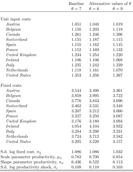
There are two parameters that cannot be estimated directly with the data at hand. I set the value of the elasticity of substitution between products,σ, to six. This implies a reasonable mark-up of 20 percent above marginal costs. The model requires the assumption thatθ > σ−1. Ifθ→σ−1 = 5, firms’ foreign production locations do not cannibalize each other at all, which is as if they were all producing distinct products. This knife-edge case clearly would be implausible empirically, as it is known for example from the car industry that the same car model is often produced in various production locations. For the baseline parameterization of the model, I set the dispersion parameter of the productivity draws, θ, to seven, which is close to the median estimate for the productivity dispersion parameter by Eaton and Kortum (2002). I show the robustness of the estimates and counterfactual results to θ= 6 and θ = 9 in the Appendix. In general θ could be estimated if a full matrix of affiliate-destination-specific sales for firms as well as a measure of source-destination-specific trade cost was available. Equation (9) would provide structure for such an estimation. In a recent paper, which builds on the model structure of this paper, Head and Mayer (2015), estimate θ = 9.2 using data on source-destination-specific car model trade flows.
3.3.2 Empirical Strategy
Before formally specifying the likelihood function, I discuss the intuition for the identification of the parameters. The econometrician observes firms’ production locations and their output at each location, as well as aggregate trade costs between countries and the market demand, Ym/Pm1−σ, in every country. Fixed costs provide an
incentive for a firm to concentrate its production in a few locations, while larger variable costs abroad reduce the output in all foreign locations in which the firm established a plant. A firm’s production volume in a country 25All these distributions have only positive support. The log-normal distribution provides a flexible functional form with
pa-rameters governing both mean and variance of the distribution. Similarly to recent models of exporting [e.g. Chaney (2008)], the assumption of Pareto distributed core productivities implies that firm sizes are Pareto distributed in the closed economy version of the model.
depends on the firm’s productivity, trade costs, the local and surrounding market potential of the country, and the set of other countries in which the firm has a plant and their characteristics. It is the comparison between foreign production and home production that identifies the variable cost via a ‘within firm’ comparison (as the core productivity of the firm is held constant). All else equal, larger unit input cost imply lower production volume in a foreign country. Given knowledge about variable costs, firm-country-specific productivity levels can be recovered from the firm-country-specific output observations (this statement is formalized in Proposition 2 below). Given other parameters and the variable costs, the identity of firms that operate a plant in a country and their productivity identify the fixed costs. Roughly, the mean of fixed costs comes from the number of plants established in a country and the dispersion parameter of the fixed cost distribution from the correlation between a firm’s number of plants and a firm’s productivity (when the variance is large, this relationship is weaker).
I continue to formally describe the estimation procedure below.
3.3.3 Constrained Maximum Likelihood Estimation
Following equation (15) from the model, we can write the probability that a firm with core productivity level φtselects location setZt as
Pr(Z=Zt|φt; ˜w, σ, µη˜, σ˜η) = Z ˜ η 1{E(Π(φt, Z, ,η˜;σ,w˜))≥E(Π(φt, Z0, ,η˜;σ,w˜)) ∀Z0∈ ZG}dF(˜η;µη˜, ση˜), (21) where the expected profits from selecting location setZ for firmtwith core productivityφtand fixed
cost draws ˜ηt are:
E(Π(φt, Z, ,η˜t;σ,w˜)) = 1 σκφ σ−1 t X m Z Ym Pm1−σ X k∈Z ( ˜wkτkm)−θθk !(σ−1)/θ dH(;σ)− X k∈Z,k6=G ˜ ηt,k. (22)
The first term in equation (22) represents expected variable profits from having production facilities in the countries contained in the location set, and the second term represents the fixed costs that the firm would have to pay. Recall that the level of fixed costs is known at the time the firm makes its decision, but the firm only learns how productive these facilities are after selecting its plants. The model attends to the possibility that, after the plants are established, the operations in every country are hit by productivity shocks whose realizations were not known to the firm when the production locations were established.26 The timing assumption simplifies the computation: the firm chooses its optimal location only conditional on its core productivity level,φt, the vector
26A supporting piece of evidence from time series data on German and Norwegian multinational firms is that the exit probability
of an affiliate is highest in the first year after it was established, which suggests that the firm learns something about the affiliate only after it was created (Gumpert, Moxnes, Ramondo, and Tintelnot (work in progress)).
of fixed cost draws, ˜ηt, and other parameters that are common across firms, ( ˜w, σ), but not also conditional on
the firm-country-specific productivity levels. As the firm has rational expectations, the dispersion parameter of the productivity shocks,σ, enters the probability of the location choice specified in (21).
Aside from the information about a firm’s chosen locations, we observe its total output in each country in which it is active. Given a parameter guess of the unit input costs across countries, we can learn about the country-specific productivities of the multinational from the country-specific output levels. Note that the productivity of firmtin countrylis the product of the core productivity level,φt, and the firm-country specific
productivity shifter, t,l. I denote this expression by ψt,l = φtt,l. Let rt,l( ˜w, Zt, ψt) = P m
slm(it, φt, Zt, t)
denote the total revenue from sales to all countries of firmtin countryl.
Rewriting equation (11) from the model using the new notation, we get the following expression for the output of firmtin countryl:
rt,l( ˜w, Zt, ψt) =κ X m Ym Pm1−σ ( ˜wlτlm)−θψθt,l P k∈Zt ( ˜wkτkm) −θ ψθ t,k !(θ+1θ−σ) . (23)
We have such an equation for every location in which firmt has a production location. Letrt denote
the vector of outputs of firmtin its production locations. Importantly, knowing the output of a firm in each of its locations and all other parameters allows us to pin down exactly its productivity level,ψt,l=φtt,l, in each
of its locationsl. Proposition 2 states that given all other parameters, the solution to this system of equations is unique (the proof is in the appendix).
Proposition 2. Let r : RK
++ × ZG ×Ψ → RK++ be the stacked vector of revenues as defined in equation (23), where K denotes the number of countries in which firm t has a plant and Ψ = [ψmin, ψmax]K with
0< ψmin< ψmax<∞. Then for any triple {rt,w, Z˜ }, the vectorψ that solvesrt−r( ˜w, Z, ψ) = 0is unique.
The likelihood function for each firm consists of the probability of its chosen location set and the density of the plant-specific revenues of the firm conditional on its location set and its core productivity level. I integrate out the core productivity level of each firm, which is observed by the firm but unobserved by the researcher. The likelihood function of the parameters Θ ={w, σ˜ , µη˜, ση˜, µφ, σφ}given the observed data on location choice
and revenues {Zt, rt}Tt=1 can be written as:
L(Θ;{Zt, rt}Tt=1) = T Y t=1 Z Pr(Z=Zt|φ; ˜w, σ, µη˜, ση˜)g(rt|Zt, φ; ˜w)dG(φ;µφ, σφ), (24)
The first factor under the integral – the probability of the location choice – is specified directly in (21). The second factor – the density of the revenues – can be expressed in terms of the density of the plant-specific
productivity shifters, t,l = ψt,l
φt . It follows from Proposition 2 that the vector of revenues, rt, can be inverted to get the vector of plant-specific productivity levels, ψt. The firm-location-specific productivity shifter t,l is
i.i.d. across firms and locations. I rewrite the likelihood function in (24) as
L(Θ;{Zt, ψt}Tt=1) = T Y t=1 Z Pr(Z =Zt|φ; ˜w, σ, µη˜, ση˜)|Jt(φ,w˜)| Y l∈Zt h ψ t,l( ˜w) φ |σ dG(φ;µφ, σφ). (25)
where h(· | σ) denotes the univariate density of the firm-location-specific productivity shifter. The term
|Jt(φ; ˜w)|is the determinant of the Jacobian, which is included in the likelihood function because of the change
of variables from the firm’s revenues to the firm’s productivity shifters.
Note that the firm-specific productivity shifter is not directly observed; we learn about the firm’s productivity level in country k – given the current parameter guess and the observed country-specific output levels of the firm – from a system of equations that contains the output of the firm in each of its locations specified in (23). Therefore, I solve the following constrained optimization problem to estimate the parameters in which the objective function is the logarithm of the likelihood function specified in (25):
max Θ,ψ logL(Θ;{Zt, ψt} T t=1) subject to: rt,l( ˜w, Zt, ψt) =κ X m Ym Pm1−σ ( ˜wlτlm)−θψt,lθ P k∈Zt ( ˜wkτkm) −θ ψθ t,k !(θ+1θ−σ) ∀t∈ {1, ...T},l∈ {1, ...N} such thatl∈Zt. (26)
In summary, I use data on the chosen set of countries,Zt, for each firmt(the probability of the location
choice is the first term of the likelihood function) and the observed output in every countryrt,l in which firmt
is active (which is the left hand side of the constraints) to estimate the following parameters: the vector of unit input costs, ˜w, the vectors that characterize the destination-country-specific distributions of fixed costs,µη˜and
ση˜, the parameters for the core productivity distribution,µφ andσφ, and the parameter that characterizes the
dispersion of the firm-country-specific productivity shocks, σ. Given the structural parameters and the vector
of location-specific outputs, the vector of the firm-country-specific productivity levels, ψ, solves the system of constraints. I control for unobserved heterogeneity in the core productivity levels of the firms and in the country-specific fixed cost draws.
3.4
Parameter Estimates
Table 1 displays the parameter estimates. I find that for German multinationals the variable costs of production (unit input costs) are systematically smaller in Germany than in foreign countries, which is not surprising given the low foreign output share abroad discussed in Section 3.2. The unit input costs in Germany are normalized to one. The smallest difference in unit input costs is found in Austria, in which German multinationals face only around five percent larger variable production costs than at home. Within Western European countries, the production costs for German multinationals are largest in Italy and the United Kingdom (23 percent higher than in Germany). The production costs in the United States are around 35 percent higher than at home. The differences in production costs reflect both wage-level differences and efficiency losses that occur by producing outside the home country. One would expect the efficiency losses to be affected by the standard gravity variables (distance, contiguity, and language) and, accordingly, the unit input costs show a tendency to rise with distance, and fall with contiguity and common language.
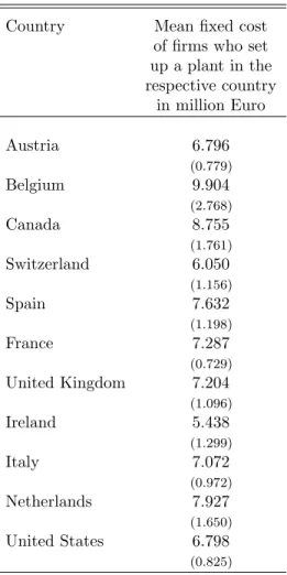
We can give the fixed costs a value interpretation as we observe the firms’ output in Euro and, with CES preferences and monopolistic competition, we can easily determine that variable profits are proportional to output. Fixed costs are identified by observing the actual choice of production locations and variable profits together with the counterfactual scenarios of how variable profits would change if the firm altered its set of production locations. Note that my model does not distinguish between fixed costs to maintain a plant and sunk costs to establish a foreign plant. I use the estimates in Table 1 together with the structure of the model to calculate the mean fixed costs paid by firms that set up a production location in the respective countries. The calculation of the mean fixed cost conditional on having established a plant in the country is described in Appendix F, and the results are displayed in Table 2. For most countries the estimated mean fixed cost of plants that were actually established is 6-8 million Euro. The paid fixed cost is estimated to be larger in Canada (8.8 million) and Belgium (9.9 million). The larger fixed cost estimates for these countries are in accordance with the data in Table 8 in Appendix B. Belgium has almost the same geographic location as the Netherlands and a similar local and surrounding market potential. While the number of German firms that have production locations in these countries is about the same, the output of affiliates in Belgium is much larger. These differences result in lower estimated variable production costs in Belgium, but larger fixed costs. The lower variable costs ensure larger firms in Belgium, while the larger fixed costs ensure that the number of predicted entrants are comparable across countries. Similarly, only a small number of firms has a plant in Canada, but they tend to have very large outputs. Unlike the unit input costs, the fixed cost estimates do not show a tendency to rise with distance from the host countries.
As discussed in the model section, the analysis in this paper abstracts away from fixed costs of market access. To conduct sensitivity analysis how the lack of fixed cost of market access may affect the estimation
Table 1: Maximum Likelihood Estimates
Unit input costs Fixed costs ˜ w µη˜ Country Austria 1.051 3.544 (0.022) (0.235) Belgium 1.150 3.859 (0.054) (0.278) Canada 1.261 3.776 (0.043) (0.222) Switzerland 1.155 3.462 (0.023) (0.243) Spain 1.155 3.207 (0.019) (0.229) France 1.152 3.227 (0.015) (0.179) United Kingdom 1.234 3.176 (0.016) (0.234) Ireland 1.106 4.054 (0.045) (0.323) Italy 1.235 3.284 (0.023) (0.221) Netherlands 1.118 3.724 (0.024) (0.246) United States 1.353 3.205 (0.023) (0.175)
S.d. log fixed cost,ση˜ 1.086
(0.107)
Scale parameter productivity,µφ 0.783
(0.003)
Shape parameter productivity,σφ 6.436
(0.313)
S.d. log productivity shock,σ 0.108
(0.005)
Log-Likelihood -9.86E+03
Number of firms,T 9288
Notes: Unit costs in Germany are normalized to one. Standard errors in parentheses.
results, I carry out the following experiment: Suppose the estimated parameters in Table 1 are the true parame-ters of the data generating process. However, in addition there would be fixed costs of market access,ιmwi = ¯ι.
I simulate data from this extended model with fixed costs of market access (see footnote 16 on how to include fixed costs of market access), and then estimate the regular model without such fixed costs of market access. If the estimated parameters are very close to the true parameters, the bias from a lack of fixed costs of market access does not seem to be severe. An obvious question is how large the fixed costs of market access should be. Bernard, Jensen, and Schott (2009) report that on average the export volume by US firms that serve only a single market was about 250k USD in year 2000. Assuming that operating profits are 20 percent of sales, it
seems unlikely that the fixed costs of market access for those firms exceeded 50k USD (which was about 52.5k Euro in year 2000), otherwise they would incur losses from exporting. I estimate the sensitivity of my parameter estimates to fixed costs of market access of 50k, 100k, 200k and 300k Euro. Table 11 in Appendix C presents the results. I find that for reasonable fixed costs of market access (50k - 100k Euro), the estimated parameters are very close to the true parameters. However for very large fixed cost of market access, the estimated parameters overstate the the cost of the foreign input bundle – making firms appear less efficient abroad than they actually are. Overall, these results suggest that for empirically plausible values of fixed marketing costs, ignoring such costs is not likely to severely affect the other parameter estimates.
I also evaluate the robustness of the parameter estimates for German multinational firms to alternative values of the parameterθ. Table 12 in Appendix C presents the results. The estimates are largely unchanged forθ= 6 andθ= 9.
Table 2: Fixed cost by country
Country Mean fixed cost
of firms who set up a plant in the respective country in million Euro Austria 6.796 (0.779) Belgium 9.904 (2.768) Canada 8.755 (1.761) Switzerland 6.050 (1.156) Spain 7.632 (1.198) France 7.287 (0.729) United Kingdom 7.204 (1.096) Ireland 5.438 (1.299) Italy 7.072 (0.972) Netherlands 7.927 (1.650) United States 6.798 (0.825)
3.5
Decomposing the sources of home bias in production
Multinational firms have been characterized as footloose and free to reorganize their global operations as the global economic environment changes [Caves (1996)].27 However, the evidence presented in Section 3.2 suggests that this view of footloose multinationals is inaccurate, and, rather, firms show ‘home bias in production.’ Fur-ther, while the copious literature on the proximity-concentration trade-off has provided evidence for the presence of fixed costs, little is known about their quantitative importance. The parameter estimates above demonstrate both significant fixed costs to starting production in a foreign country and higher variable production costs abroad. In order to learn more about the quantitative importance of each of those barriers, in this section, I let firms re-optimize their location decisions as well as their decisions about which market to serve from which location, under different fixed and variable costs. I hold general equilibrium variables such as income and price indices fixed as I change the cost parameters.
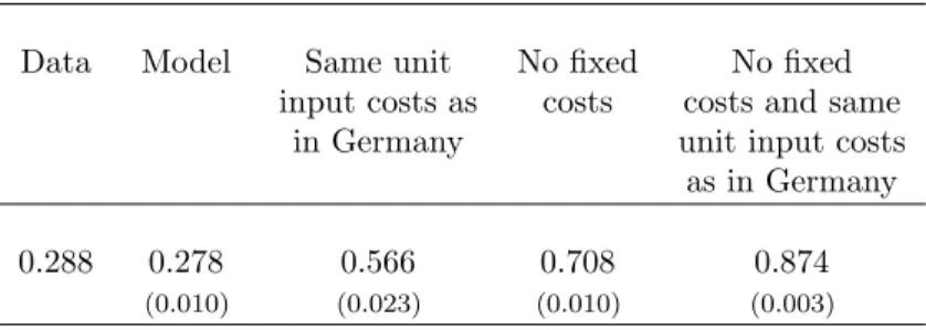
Table 3 contains the results. The model effectively fits the average share of foreign output across firms. While in the data the average foreign output share is 0.29, in the estimated model the average foreign output share is 0.28 percent. If the unit input costs in the foreign countries were the same as in Germany, and there were no fixed costs for setting up foreign plants, then every firm would have a plant in each country, and the average foreign output share across firms would be 0.87. The question arises as to whether fixed costs or larger variable production costs abroad are the more important barrier to foreign production. If unit input costs were equalized across countries, and fixed costs were kept at their estimated level, then firms would re-optimize their production locations and output decisions such that the foreign output share would be 0.57. If, instead, fixed costs were eliminated (and unit input costs held at their estimated level), the average foreign output share would rise even further to 0.71. Overall, I find that both fixed costs and differences in unit input costs significantly contribute to home bias in production. While both factors have a large quantitative effect, fixed costs are slightly more important.
Table 3: Average share of foreign production in the
output of German multinationals
Data Model Same unit No fixed No fixed
input costs as costs costs and same
in Germany unit input costs
as in Germany
0.288 0.278 0.566 0.708 0.874
(0.010) (0.023) (0.010) (0.003)
Notes: Trade costs and price indices are held fixed. Standard errors in parentheses.
4
Calibration
In the second tier of my empirical inquiry, I focus on general equilibrium welfare analysis. In this section, I calibrate the key parameters to the general equilibrium outcomes of the model using data for many countries. Specifically, I calibrate trade costs, variable foreign production costs, and fixed costs of setting up foreign affiliates, to data on bilateral trade flows, the values of output of firms from country i in country l, and the estimates of the country-specific variable production costs of German multinationals from the previous section. The estimates of fixed and variable production costs for German multinationals from the previous section enable me to include both variable foreign production frictions and fixed costs in the analysis. On the aggregate level, both fixed costs of establishing foreign locations and higher variable production costs abroad discourage foreign production, so separating the two barriers would be infeasible with information only about aggregate flows. I solve for the endogenous relative wages and price indices in every country.
4.1
Additional Data
The analysis incorporates the same twelve Western European and North American countries as the previous sec-tion. Data on multinational production comes from Ramondo, Rodr´ıguez-Clare, and Tintelnot (2015).28 Gross manufacturing production and bilateral trade data comes from OECD STAN, and figures on labor endowments are drawn from the Penn World Tables. Data on trade and multinational production (MP) are averages across the years 1996 to 2001, and the figures on population are for the year 2000.
4.2
Calibration procedure
The model delivers predictions for MP and trade shares, which I use as moments to calibrate the parameters.29 The share of expenditures by consumers from country mthat is spent on goods produced in country l (‘trade share’) is
ξlm=
Xlm
Ym
, (27)
and the share of output produced by firms from countryiin countryl (‘MP share’) is
κil= P m Xilm P m Xlm . (28)
28Unlike bilateral trade flow data, data on production activities of multinationals in foreign countries is documented only
sporad-ically. Ramondo, Rodr´ıguez-Clare, and Tintelnot (2015) construct a data set using data from UNCTAD on non-financial affiliate sales by firms from countryiproducing in countryl. Since many of the country-pairs’ observations are missing, they interpolate missing values using a regression of affiliate sales on the stock of M&A between these countries (which is available for a wider set of country-pairs). For the selected set of countries used in this paper, only 17 out of 132 country-pairs’ MP values in Ramondo, Rodr´ıguez-Clare, and Tintelnot (2015) were obtained via interpolation.
The share of purchases of domestically produced goods and the share of production carried out by local firms are included in these moments above. As an additional set of moments, I include the relative unit input costs of German firms in various countries that were estimated in Section 3. These are driven both by the foreign efficiency losses, γ, and endogenous relative wages, w. Relative variable production costs for German (G) firms in country l are wlγGl
wG . Let ˜wG denote the vector of such relative production costs for German firms and ˆw˜G denote their estimates based on the German micro data in the previous section. The calibration
procedure (formally described below in (29)) aims to bring these expressions – as well as the MP share and trade shares in the model and data– close to each other while simultaneously solving for endogenous wages by solving the equilibrium constraints. Note that I do not impose the restriction that multinational firms from other countries have the same variable production costs as German firms in the foreign host countries. Rather, as specificed below, the variable effiency losses of multinational firms producing abroad are imposed to follow a gravity pattern.30
I estimate the parameters that characterize the trade costs between countriesl andm, τlm; efficiency
losses of foreign production,γil; and the distribution of fixed costs to set up plants in foreign countries as a firm
from countryi,Fi(η). I make the following restrictions on the functional form for trade and foreign production
iceberg costs: τlm = βconstτ (distlm)β τ dist(βτ contig) contiglm(βτ lang) languagelm forl6=m γil = β γ const(distil)β γ dist(βγ contig) contigil(βγ lang) languageil fori6=