UPCommons
Portal del coneixement obert de la UPC
http://upcommons.upc.edu/e-prints
Aquesta és una còpia de la versió
author’s final draft
d'un article
publicat a la revista
Energy Policy
.
URL d'aquest document a UPCommons E-prints:
https://upcommons.upc.edu/handle/2117/119594
Article publicat / Published paper:
Sala, E., Delgado Prieto, M., Kampouropoulos, K., Romeral, L.
Activity-aware HVAC power demand forecasting. "Energy and
buildings", 1 Juliol 2018, vol. 170, p. 15-24. DOI:
10.1016/j.enbuild.2018.03.087
© 2016. Aquesta versió està disponible sota la llicència CC-BY-NCND
3.0
http://creativecommons.org/licenses/by-nc-nd/3.0/es/
Activity-Aware HVAC Power Demand Forecasting
1Abstract – The forecasting of the thermal power demand is essential to support the development of advanced strategies
2
for the management of local resources on the consumer side, such as heating ventilation and air conditioning (HVAC)
3
equipment in buildings. In this paper, a novel hybrid methodology is presented for the short-term load forecasting of
4
HVAC thermal power demand in smart buildings based on a data-driven approach. The methodology implements an
5
estimation of the building’s activity in order to improve the dynamics responsiveness and context awareness of the
6
demand prediction system, thus improving its accuracy by taking into account the usage pattern of the building. A
7
dedicated activity prediction model supported by a recurrent neural network is built considering this specific indicator,
8
which is then integrated with a power demand model built with an adaptive neuro-fuzzy inference system. Since the
9
power demand is not directly available, an estimation method is proposed, which permits the indirect monitoring of the
10
aggregated power consumption of the terminal units. The presented methodology is validated experimentally in terms of
11
accuracy and performance using real data from a research building, showing that the accuracy of the power prediction
12
can be improved when using a specialized modeling structure to estimate the building’s activity.
13
Keywords – energy management systems, load prediction, machine learning, neural networks, smart buildings.
14
Nomenclature:
15
ABM Agent-Based Modeling
AHU Air Handling Unit
ANFIS Adaptive Neuro-Fuzzy Inference System
BEMS Building Energy Management System
DSM Demand-Side Management
HMM Hidden Markov Model
HVAC Heating Ventilating and Air Conditioning
MAE Mean Average Error
MAPE Mean Absolute Percentage Error
MAX Maximum Error
OPC Open Platform Communications
R2 Coefficient of Determination
RMSE Root Mean Squared Error
RNN Recurrent Neural Network
SCADA Supervisory Control and Data Acquisition
1.
Introduction
16
1.1
Background and motivation
17
Recent advances in the functionalities of modern Building Energy Management Systems (BEMS) in terms of 18
monitoring and supervision [1, 2] have paved the way in the framework of smart buildings for the introduction of Demand-19
Side Management (DSM) practices [3], which are one of the most important methods for achieving energy savings [4]. The 20
increased insight derived from this progress has been instrumental in the further study of context-aware solutions that are 21
capable of improving the energy efficiency of technical services in BEMS by building on the expanded knowledge 22
available [5]. By accounting for up to 40% of the power consumed in buildings, heating ventilating and air conditioning 23
(HVAC) systems, in particular, have attracted a substantial share of current research efforts [6, 7]. 24
In modern buildings, load modeling and forecasting methodologies able to predict the future power demand of HVAC 25
systems are an important concern of installation managers due to the useful knowledge that they provide [8], since real-26
time demand information plays a role in mitigating energy waste [9]. Several types of methodologies exist, being data-27
driven approaches the most prevalent. However, when applied to HVAC systems, these methodologies are mostly aimed at 28
forecasting the consumption load [10]. Instead, focusing on the thermal power demand may help abstract from 29
performance differences caused by regulation systems and to better reflect the power needs of the facility. Automation 30
systems can benefit from this information in order to make decisions autonomously by following energy-saving 31
optimization strategies. This is especially true for the control of HVAC equipment, where the predicted load could be used 32
for implementing model-predictive control strategies. Multiple control approaches applied to HVAC systems that could 33
benefit from this information can be found in the literature, such as the planning of energy storage during off-peak periods 34
using cooling storage systems [11]. Others also include the planning of adequate startup and shutdown times for heating 35
and cooling equipment in order to save energy by meeting the right amount of power demands, and for the orchestration of 36
machine actuations in installations where multiple machines are available [12]. Furthermore, the combination of HVAC 37
load forecasting with machinery efficiency maps, represents an underexploited avenue of improvement with a high 38
potential for the optimization of the operation of the system. That is, the demand anticipation and the utilization of the most 39
suitable machine for each situation would provide a positive affectation to the overall equipment’s performance, which is a 40
significant present-day problem in building management and maintenance. Indeed, the overall efficiency of the installation 41
could be improved, since the current most common method for allocation HVAC capacity is based on setting the same 42
water temperature thresholds on all the available machines [13]. 43
Even though this framework represents one of the main current research interests stated by the related scientific 44
community, the obstacles for its implementation are double-sided. First, the efficiency maps are difficult to obtain when 45
precision beyond the manufacturer’s sparse figures is desired, as they would require extensive testing of the unit in each 46
installation, and would likely drift over time as the equipment deteriorates with aging. Secondly, the methodologies for 47
obtaining load predictions in HVAC systems are not mature enough and their implementation can be quite challenging due 48
to the potential complexity of energy systems [14]. 49
1.2
Literature review
50
In the recent literature, considerable scientific effort has been committed to the research of load forecasting algorithms 51
and methodologies, as seen in the latest review papers [15]. A comprehensive review of more than one hundred papers on 52
electrical load forecasting defined a general taxonomy for selecting modeling algorithms from the point of view of their 53
popularity in different applications, indicating that data-driven approaches are mainly used in short-term forecasting 54
applications due to their complex dynamics [16]. In contrast, a comparative analysis studied eleven modeling algorithms 55
from the point of view of their performance when applied to the same dataset, revealing their applicability in different 56
scenarios including cases with limited data or high variability [17]. However, even though numerous general-purpose 57
approaches exist for the implementation of load forecasting, their limitations are revealed when applied to real HVAC 58
systems, which are mainly related to the difficulty of adapting the predictions to the power demand changes caused by 59
fluctuations of influencing parameters, such as the weather and the occupant’s behavior during the day [8]. 60
In this regard, recent studies as the one presented by M. Peña et al. in [18], confirm the significant correlation between
61
the occupancy of the building’s spaces and the HVAC equipment’s actuations and consequent operational regime changes. 62
This, as promoted by different authors, as T. Hong et al. in [19], indicates that the occupancy should be a key aspect in the
63
research of energy usage in buildings, because of its potential contributions to efficiency improvements. Actually, a recent 64
review of energy efficient ventilation strategies concluded that large amounts of energy are being wasted because of 65
conditioning building areas that have effectively empty periods of time, and that accounting for these may help to greatly 66
increase efficiency [20]. Indeed, most of the current load simulation and forecasting methodologies show a lack of 67
occupancy awareness, while the available studies dealing with the integration of occupancy data into load forecasting 68
systems to enhance the accuracy of power demand predictions present critical limitations and insufficient proficiency [21]. 69
Similarly, a recent review of artificial intelligence methods for load forecasting in buildings suggested that the 70
integration of occupancy data has the potential for improving energy predictions [22]. Moreover, it was stated by J. 71
Massana et al. in a study of the application of neural networks for building energy forecasting, that occupancy-based inputs
72
should be taken into consideration in future studies because of the impact that the occupancy can have on the building’s 73
thermal energy usage. This is shown in [23] and further developed in [24], where several attributes were studied, 74
concluding that it would be useful to create occupancy indicators for improving the prediction capabilities. 75
On this subject, some methodologies for the modelling and forecasting of occupancy in buildings exist, being Agent-76
Based Modelling (ABM), and Hidden Markov Models (HHMs) the most common. ABM approaches try to mimic the 77
behavior of occupants within a building in order to simulate either occupancy patterns or their effects at the occupant level 78
[25], hence being too fine-grained for full building applications. Alternately, HMMs are stochastic processes that naturally 79
fit the problem of modelling occupancy patterns, because they treat occupancy as a series of transitions between states and 80
attempt to estimate and simulate the probabilities of transitions among such states [26]. HMMs are useful at low 81
aggregation levels, for example for assessing the probability of a given space becoming occupied, but are not a good fit for 82
big scenarios, as the complexity grows exponentially with the number of zones [27]. Another disadvantage of HMMs at 83
high aggregation levels is that their future state is a function of their current state, not taking into consideration past states. 84
This property could neglect important features of the aggregated occupancy, such as the ratio of change. Indeed, complete 85
and viable solutions are yet to be investigated, and the proper way to monitor the occupancy, to define the indicators and to 86
integrate them into a load forecasting system remain to be established. 87
1.3
Innovative contribution
88
In this paper, an HVAC thermal power demand forecasting methodology composed by the integration of a power 89
demand model and an activity indicator model is studied. The methodology aims to extract the occupancy patterns in order 90
to determine the level of activity in the building and thus to improve the accuracy of the power demand forecasting. With 91
this objective, the building’s historical database is divided into occupancy and load data for separate preprocessing. Then, 92
an activity indicator is built and a model is implemented using Recurrent Neural Networks (RNN) to enhance the 93
consideration of dynamic temporal patterns, while the power demand characterization is carried out by means of a state-of-94
the-art Adaptive Neuro-Fuzzy Inference System (ANFIS) structure. Finally, a reliable and robust power demand 95
forecasting model is obtained by the serialized fusion of both inference systems. 96
The main contribution of this study lies in a new data-driven short-term load forecasting methodology for the prediction 97
of the thermal power demand of HVAC systems in buildings, and the introduction and verification of an activity indicator 98
estimation procedure to support the prediction of the power demand. 99
Aligned with the current research challenges in the field, the methodology takes advantage of real-time occupancy data 100
in order to predict an activity indicator, providing accurate insight regarding the thermal needs of the building in terms of 101
the volume of consumption endpoints in operation. Furthermore, due to the difficulty in directly measuring the thermal 102
power demand signal, which would involve the use of extensive instrumentation installed in consumption endpoints 103
throughout the building, an estimation method is proposed in order to calculate the actual power draw, derived from the 104
measurement of the thermal power output of the HVAC energy production equipment in the building. The novelty of this 105
work includes the implementation of a new hybrid solution that offers major advantages over traditional approaches. In 106
particular, the collaborative model structure, comprehending the separate modeling of the activity indicator’s dynamics and 107
the thermal power demand characterization, differs from classical single model approaches in that it allows the selection, 108
tuning and fitting of each structure independently, increasing its adaptability to the dynamics of each signal and improving 109
the resulting accuracy through the specialization of its modeling process. It should be noted that this is the first time that 110
this methodology as well as this activity indicator modelling is used in building automation and energy management for 111
providing accurate insight regarding the thermal needs of the building, with the objective of supporting the enhancement of 112
resource management and the optimization of the operation of local equipment. 113
This paper is organized as follows. Section II presents the proposed methodology, focusing on the occupancy 114
monitoring to create an activity indicator, the thermal demand estimation of the HVAC system and the load forecasting that 115
merges this information in order to calculate predictions. Section III describes the test environment. Section IV shows the 116
experimental results obtained from the implementation and validation in a real building. Finally, the conclusions of this 117
work are drawn in Section V. 118
2.
Proposed Methodology
119
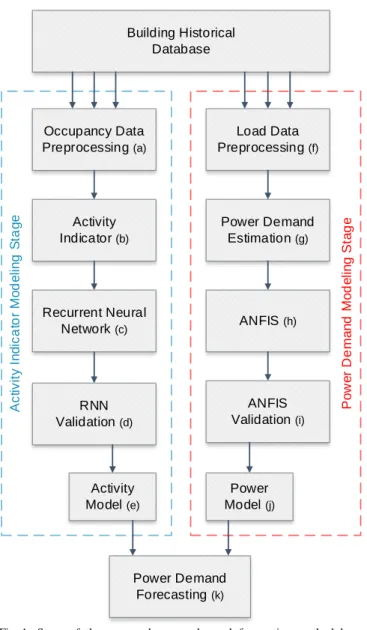
A step-by-step diagram of the complete methodology is shown in Fig. 1, which is divided into three stages: the activity 120
indicator modeling stage, where an artificial activity indicator is defined and modelled, the power demand modeling stage, 121
where the power demand of the HVAC system is estimated and modelled separately and finally the demand forecasting 122
stage, where predictions are obtained by means of the evaluation of the models. 123
124
Initially, on the activity indicator modeling stage, the occupancy data is extracted from the building’s historical 125
database and is preprocessed in order to remove gaps due to acquisition interruptions, outliers and erroneous readings (a). 126
The activity indicator is then defined as the aggregation of the binary occupancy signals (b) and the obtained indicator is 127
modeled by means of a recurrent neural network with global feedback (c). The trained network’s performance is evaluated 128
over a test dataset in order to validate that it has properly learned the indicator’s behavior (d). 129
Afterwards, during the power demand modeling stage, power data plus auxiliary signals are loaded and preprocessed in 130
a similar manner (f). Then, a power demand estimation method (g) allows the calculation of the total power demand 131
corresponding to the consumption endpoints in the building, decoupling the effect of the distribution bus capacity and the 132
control strategy. Next, an ANFIS model is built for the forecasting of the obtained thermal power consumption signal by 133
selecting the most suitable set of input variables and training the inference structure (h). After the model is trained, it is 134
validated (i) in a similar manner as the activity indicator model in order to ensure its accuracy. 135
Finally, the activity indicator model (e) is combined with the obtained power demand model (j) to support the 136
calculation of power demand predictions (k). The combination is performed in series, where the output of the activity 137
model is used as an input of the power model. 138
The following subsections describe the main stages of the methodology in detail. 139
2.1
Activity indicator modeling
140
In the literature, some studies use timetables as a rough estimation of occupancy, exploring the potential energy savings 141
that could be achieved by implementing management strategies that take advantage of personalized occupancy schedules 142
[28], schedules of the temperature settings of the building [29], or occupancy patterns derived by mining the energy 143
consumption of appliances [30]. However, a recent review of occupancy modeling approaches concluded that schedule-144
based methodologies are not suitable for applications aimed at improving energy efficiency in buildings, in favor of more 145 P ow er D e m and M od el ing S tag e Occupancy Data Preprocessing (a) Activity Indicator (b) Recurrent Neural Network (c) RNN Validation (d) A c tiv it y I ndi c a to r M od el ing S ta ge Load Data Preprocessing (f) Power Demand Estimation (g) ANFIS (h) ANFIS Validation (i) Activity Model (e) Power Model (j) Building Historical Database Power Demand Forecasting (k)
Fig 1. Steps of the proposed power demand forecasting methodology divided into activity modeling stage and power demand modeling stage.
sophisticated methods that are able to learn and predict the behavior of occupants [21]. Accordingly, the implementation of 146
a new model of the occupancy pattern of a building is introduced in this methodology. 147
Thus, in the proposed methodology the concept of an activity indicator is introduced with the aim of incorporating the 148
information relating to the occupancy of the building into the load forecasting system. The proposed activity indicator is 149
defined as the percentage of active spaces in a building, given that the spaces are monitored with presence detectors, which 150
are common in modern buildings for climate and lighting control purposes. The percentage of active spaces is not intended 151
to be a direct measurement of the occupation as the number of present occupants, instead it is used as a measurement of the 152
amount of activity in the building in terms of spaces where the HVAC system is in operation. The integration of this 153
indicator into the load forecasting system may lead to more accurate predictions, because the amount of rooms with an 154
operating local air handling unit (AHU) is likely to significantly affect the load of the HVAC equipment (chillers, heat 155
pumps, etc.) at the energy production stage. However, information regarding this or any other artificial activity indicator is 156
unknown beforehand, as opposed to variables such as weather conditions, which can be pulled from a local weather service 157
with reasonable accuracy. In consequence, a dedicated activity modeling system is integrated into the methodology in order 158
to independently obtain a model of the dynamics of this signal so it can be used for improving the accuracy of the 159
subsequent power demand forecasting. 160
The modeling of the activity indicator is based on a RNN, which is a data-driven technique that is well suited for cases 161
where the target signal does not present a direct correlation with other signals that could have been used as model inputs, 162
and instead depends on learning the target signal’s own dynamics. This is possible because RNNs introduce the time 163
element through their internal states, which allow the network to remember information about the past and to use it for the 164
calculation of predictions, facilitating the learning of the temporal dynamics of the target, instead of relying solely on the 165
current inputs [31]. This feature of RNNs makes them suitable for modelling the activity indicator, which is not strongly 166
correlated with other signals, thus the modeling relies on accumulated state for learning its temporal dynamics, in this case 167
complemented with the time of the day and the day of the week for increased robustness. Additionally, memory units have 168
been incorporated into the network in order to provide auto-regressive behavior; this allows the network to not only take 169
into account the previous recurrent state, but past states as well. 170
The RNN is trained in open-loop form by means of backpropagation, where its coefficients are tuned with the objective 171
function corresponding to the minimization of the mean-squared error of the prediction of the state of the next iteration. 172
After the modeling process is carried out using the open-loop network, the feedback loop is closed to allow the calculation 173
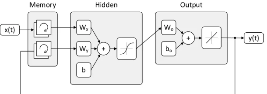
of predictions taking advantage of the recurrent nature of the network. Using the closed-loop form, prediction iterations are 174
calculated based on the value of the previous state, the inputs and past states provided by the memory units,. The structure 175
of the complete closed-loop RNN is shown in Fig 2. The trained network is then validated in terms of accuracy using 176
several error metrics, evaluating its performance as more iterations are calculated. The results of the validation ascertain 177
whether the performance is sufficient at the desired prediction horizon. 178
179
2.2
Power demand modeling
180
The implementation of the power demand model begins with the initial step of preprocessing the signals to interpolate 181
possible gaps and filter noisy signals acquired by sensors. In addition, a final step is considered for the validation of the 182
trained model structure. However, the core of the proposed power demand modelling is composed of the following two 183
main steps: the power demand estimation, and the fitting of the ANFIS model. 184
2.2.1
Power demand estimation
185
The power consumption of HVAC systems is a form of instrumentation that is frequently found in buildings, especially 186
in modern smart buildings that incorporate BEMS, which are the main target environment of novel methodology proposals. 187
Thermal power demand, however, is not a variable that is commonly monitored directly due to the high cost of installing 188
sensors in consumption endpoints, even though it is the most useful signal to support the optimization of local resources. 189
The reasoning is based on the fact that when load forecasting systems are implemented for demand response programs or 190
other applications in the context of the smart grid, it makes sense to provide the power consumption of the complete 191
system, because these applications are focused on the optimization and planning of upstream resources. Instead, the 192
proposed method is aimed at providing a forecasting model of the thermal power demand, which can be used to optimize 193
the operation of on-site resources such as HVAC machines. 194 Wo bo + Output Hidden Memory Wx Wy + b x(t) y(t)
Fig 2. Structure of the closed-loop recurrent neural network, composed by an input layer with memory units, a hidden layer, and an output layer with a feedback loop.
Since directly measuring the thermal power consumption of the building in real-time is not a commonly affordable 195
option, which would limit the applicability and impact of the methodology, an indirect solution is proposed. The method 196
follows a grey-box approach to allow the estimation of the power demand observed in the thermal distribution bus of the 197
building, implemented as described next. 198
The energy balance of the bus (1) is calculated for each time sample, where 𝑄𝑄𝑖𝑖𝑖𝑖 is the thermal power produced by the
199
HVAC equipment, measured using an ultrasonic flow meter plus a differential temperature sensor, and Qout is the power
200
drawn from the bus, which is not known. The energy accumulated in the bus Qbus during each cycle is described by (2)
201
where Cp is the specific heat of the fluid in the bus, ∆Tbus is the increment of the temperature of the bus, and m is the total
202
mass of the fluid. 203
204 205 206 207
Once the energy balance is defined by the input energy flow 𝑄𝑄𝑖𝑖𝑖𝑖 and the energy accumulated in the bus Qbus, the
208
resulting power flow being drawn by the consumption endpoints Qout can be calculated by subtraction.
209
2.2.2
Power demand model fitting
210
After the thermal power demand is obtained, a forecasting model is built for this new signal. The method used in this 211
study for the implementation of the load forecasting is the Adaptive Neuro-Fuzzy Inference System (ANFIS). Even though 212
neural networks are the most popular data-driven methods, mainly due to their accuracy and non-linear mapping 213
capabilities [32], they present drawbacks such as falling on local minima and requiring large datasets [33]. Instead, ANFIS 214
combines the advantages of neural networks with fuzzy systems to better handle complex and adaptive systems, having 215
been validated in multiple load forecasting studies [34]. 216
For the implementation of the ANFIS model, several input signal candidates are considered besides the previously built 217
activity indicator, including weather parameters and other variables commonly available in BEMS, as described in the test 218
environment section. In order to select the a set of signals that allows the proper characterization of the power demand, an 219
input selection process is carried out, which is based on the cross-correlation analysis between each of the input candidates 220
and the target signal to rule out uncorrelated signals, and the study of their dynamics by means of the frequency analysis of 221
each variable. Having considered the candidate inputs and obtained the final selection, an ANFIS model is trained and then 222
evaluated using common performance indicators: the Root Mean Squared Error (RMSE), the Mean Absolute Percentage 223
Error (MAPE), the Mean Absolute Error (MAE), the Determination Coefficient (R2) and the Maximum Error (MAX).
224
2.3
Power demand forecasting
225
Finally, the power demand of the HVAC system of the building can be predicted using the combination of the trained 226
models obtained following the previous steps. The activity indicator model provides a measure of the future occupancy 227
level, which drives the HVAC power. Then, the expected power demand is calculated to obtain the final prediction, 228
corresponding to this activity and the other influencing variables. In summary, the obtained models are combined in series, 229
with the activity indicator forecast being fed to the power demand model to calculate the final prediction. 230
Besides the activity indicator estimation procedure, the hybrid solution adopted in this study offers several advantages 231
over traditional approaches. Namely, instead of fitting a single model using a general-purpose tool, a collaborative and 232
modular structure is proposed based on specialized models built for the activity and for the power demand. Such solution 233
allows to fit and tune each method independently, adapting it to the dynamics of each signal and allowing to separately 234
train the models with the use of different datasets. 235
3.
Test Environment
236
For the validation of the proposed methodology, the complete system has been implemented in a real building in Spain. 237
The building is a research ecosystem of the Universitat Politècnica de Catalunya – BarcelonaTech, which consists of 238
offices and laboratories with a surface of 2.400m2. The environment accommodates several research groups that specialize
239
in the fields of energy efficiency, electronics, automatics, and biotechnology, among others. In this regard, the nature of the 240
tasks carried out by the staff adds a degree of additional variability to the usage patterns of the building, thus increasing the 241
complexity of the forecasting. 242
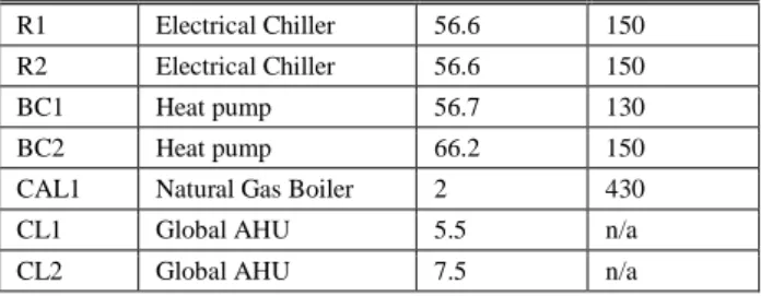
The building has several HVAC machines to be able to maintain appropriate comfort levels, including energy 243
production equipment such as chillers and heat pumps, and distribution AHUs for pre-conditioning and air renewal. 244
Additionally, the installation includes terminal AHUs that service each of the spaces in the building, with spaces having 245
multiple AHUs depending on their surface. The characteristics of these machines are shown in Table I. 246
TABLE I SUMMARY OF HVACMACHINES IN THE TEST BUILDING.
247
Id Type Pelec [kW] Pthermal [kW]
∆𝑄𝑄𝑏𝑏𝑏𝑏𝑏𝑏 =𝑄𝑄𝑖𝑖𝑖𝑖(𝑡𝑡)− 𝑄𝑄𝑜𝑜𝑏𝑏𝑜𝑜(𝑡𝑡) (1) 𝑄𝑄𝑏𝑏𝑏𝑏𝑏𝑏 =𝐶𝐶𝑝𝑝·𝑚𝑚·∆𝑇𝑇𝑏𝑏𝑏𝑏𝑏𝑏 (2)
R1 Electrical Chiller 56.6 150
R2 Electrical Chiller 56.6 150
BC1 Heat pump 56.7 130
BC2 Heat pump 66.2 150
CAL1 Natural Gas Boiler 2 430
CL1 Global AHU 5.5 n/a
CL2 Global AHU 7.5 n/a
248
In order to operate the equipment, a Modbus communication bus reads status variables such as temperatures and 249
operation modes and delivers control signals to the HVAC installation, including the production and distribution 250
equipment. Additionally, the building has an OPC server with a SCADA that centralized other sensors, including a local 251
weather station and sensors from each of the rooms and spaces in the building. The control of the HVAC system is 252
performed through the SCADA, which supports manually setting up priorities and schedules for the machines as well as 253
supervising their state in real time. 254
The test building includes a total of 130 terminal AHUs, 60 of those installed in offices, meeting rooms and 255
laboratories, and the rest in common areas. These units are wired to passive infrared presence detectors and use their 256
feedback for the regulation of the temperature in each space, which allows the fine-grained control of the internal 257
temperatures in the building. Each space is allowed to define its own comfort range, within global constraints. 258
Two separate datasets are used for the experimental validation of the proposed methodology. For the activity indicator 259
model, the available dataset comprises 8 months of data, sampled with an acquisition period of 4 minutes, from March to 260
October of 2016, including the individual occupancy signal of each of the spaces of the building. Separately, the dataset for 261
the power demand model comprises 11 weeks of data, sampled with an acquisition period of 4 minutes, from late June to 262
early September of 2016, as the dataset corresponds to the cooling power demand, which is only relevant during summer. 263
The power demand dataset contains the power output of the energy production equipment, the bus impulsion and return 264
temperatures, and the external temperature and solar irradiation, measured by the weather station. The comprehensive list 265
of available signals is shown in the following table. 266
TABLE II SUMMARY OF SIGNALS AVAILABLE IN THIS STUDY.
267
Name Description
Pth Aggregate thermal power from the energy meter.
Timp Bus impulsion temperature.
Tret Bus return temperature.
Text Outdoor temperature.
Sol Solar irradiation.
Occx Presence detector signals (x: 1, 2, 3, etc).
Act Artificial activity indicator.
268
The forecasting horizon is set to one hour in this case, as a shorter horizon would limit the applicability of the load 269
forecasting methodology, and would not allow optimization systems to plan actions with sufficient foresight. Furthermore, 270
a one-hour forecast horizon is sufficient to adapt the predictions to the significant dynamics observed in the building’s 271
datasets, which are in the range of two to three hours. 272
4.
Experimental Results
273
This section shows the implementation of the proposed methodology and discusses the obtained experimental results in 274
the described test environment. 275
4.1
Activity indicator modeling
276
After the preprocessing of the dataset’s signals to remove gaps and to filter out erroneous out-of-range samples, the 277
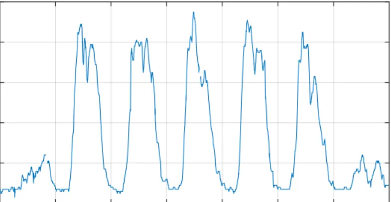
activity indicator is built using the sum of the individual occupancy signals obtained from the presence detector associated 278
to each space. The resulting activity indicator is shown in Fig 3. The pattern presented by the resulting signal follows an 279
expected trend, the indicator rises in the morning as more spaces in the building become occupied and their presence 280
detector is triggered, some drops are observed at midday as people leave for lunch, and finally most people leave during the 281
evening. However, being a research facility, some remnant occupation can routinely be observed in the building, even 282
during nighttime. 283
284
Next, the activity indicator model is built using a RNN, which must be configured before the training. The parameters 285
to be configured are the time step between the recurrent iterations, the number of memory units on the inputs and on the 286
output feedback loop, and finally the number of neurons in the hidden layer. 287
Considering the temporal aspect of RNNs, it is necessary to properly configure the iteration time step according to the 288
dynamics present in the signal and the desired prediction horizon. Thus, a small time step value in the range of minutes is 289
required in order to capture the dynamics for the next hour horizon. Further experimentation was performed in order to 290
characterize the effect of increasing the iteration time step value. This improves the performance of the network when 291
predicting the activity indicator several hours ahead. In fact, it was possible to predict the activity of the next 8 hours with 292
slightly over 10% RMSE. However, even though increasing the time step lead to expanding the forecasting horizon where 293
the model was still usable, the performance decreased in the short-term, which is precisely when maximum performance is 294
required in order to feed the power demand model. Thus, the value of the iteration time step of the RNN was configured at 295
4 minutes, which is the minimum acquisition-step available in this case. 296
Regarding the number of memory units, this amount is set to zero for the inputs, since the dynamics of the input signals 297
of the activity indicator model, which are the day of the week and the time of the day, are not relevant. Instead, the number 298
of memory units in the output feedback loop is set to 15, which at 4 minutes per iteration step matches the one hour 299
forecasting horizon desired. Therefore, the past states in the last hour are used when forecasting the next hour. Additional 300
experiments were conducted, confirming that including too few units resulted in poor performance, while including too 301
many units did not improve the prediction accuracy, but severely increased the training time due to the added parameters. 302
Concerning the amount of neurons in the hidden layer, related studies recommend using a number of neurons bigger 303
than the number of inputs in order to contribute to an information expansion prior to the output convergence. Subsequently, 304
further empirical experiments were carried out in order to select an optimal configuration. An amount of 16 neurons is 305
finally selected for the hidden layer, as fewer neurons were not able to fully estimate the dynamics of the signal, and more 306
neurons increased the training time while actually decreasing performance. 307
After the training of the network with the selected configuration, the performance of the resulting model was evaluated 308
over a reserved validation dataset, which accounted for 30% of the available data. The selected performance indicators are 309
the defined for the power demand model: the root-mean-square error (RMSE), the mean absolute percentage error 310
(MAPE), the mean average error (MAE), the maximum error (MAX) and the coefficient of determination (R2). Because of
311
the iterative nature of the evaluation of the recurrent network, where each prediction is fed back into the model to generate 312
the next state, it is not enough to evaluate the forecasting performance of a single step, as the error is accumulated at each 313
iteration. Thus, the multi-iteration performance must be evaluated to find out if the model is suitable. Fig. 4 shows the 314
progression of the selected performance indicators as the prediction horizon is expanded. As it can be observed, all of the 315
considered error indicators exhibit a performance decrease as more iterations are applied to the RNN. At 1-hour prediction 316
horizon the mean absolute error is 2.3%, which is a very accurate response taking into account the apparent random 317
behavior of the occupancy in buildings, therefore the model is deemed acceptable for the further implementation of the 318
methodology. It is also observed that the evaluation time increases in a linear trend as more feedback loops are applied in 319
order to increase the prediction horizon. 320
Fig 3. Activity indicator estimated from the aggregate of the individual occupancy signals during a week in March of 2016.
Mar 07 Mar 08 Mar 09 Mar 10 Mar 11 Mar 12
0 0.2 0.4 0.6 0.8 1 Activity Indicator
321
4.2
Power demand modeling
322
Having accomplished the activity indicator modeling stage and having obtained an activity model suitable for use, the 323
next step is to carry out the power demand modeling stage, where the activity forecasting is integrated with ANFIS in order 324
to model the power demand of the HVAC system. 325
A dataset was extracted from the building’s historical database, comprising the variables defined in the test 326
environment section. After the preprocessing of these signals, the first step was to calculate the power demand signal from 327
the measured power output of the machines and the bus temperatures by means of the estimation of the bus dynamic 328
behavior. The bus temperature signals and the estimated power demand compared to the measured power production are 329
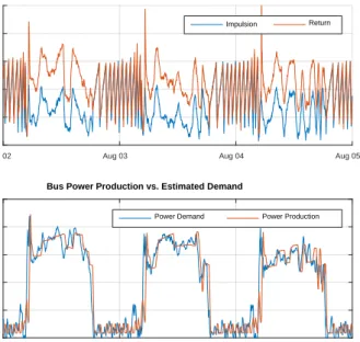
shown in Fig 5 for a period of three days in August. 330
331
Fig 4. Performance of the activity indicator model when used for multi-iteration predictions using the validation set. Root mean squared error, RMSE. Mean absolute percentage error, MAPE. Mean absolute error,
MAE. Maximum error, MAX. Determination coefficient, R2. Evaluation
time. 0 1 2 3 4 0 5 10 RMSE [%] 0 1 2 3 4 0 50 100 MAPE [%] 0 1 2 3 4 0 5 10 MAE [%] 0 1 2 3 4 0 50 100 MAX [%] 0 1 2 3 4 Time [hours] 0.9 0.95 1 R2 0 1 2 3 4 Time [hours] 46 48 50 52 Time [ms]
Fig 5. Normalized power demand signal drivers. a) Bus impulsion and return temperatures. b) Bus power production and estimated demand.
Aug 02 Aug 03 Aug 04 Aug 05 0 0.2 0.4 0.6 0.8 1
Bus Differential Temperature
Impulsion Return
Aug 02 Aug 03 Aug 04 Aug 05 0 0.2 0.4 0.6 0.8 1
Bus Power Production vs. Estimated Demand
As it can be observed in Fig. 5(b), the power demand signal, corresponding to the aggregated power drawn by the 332
consumption endpoints in the building, presents higher dynamics than the power production, corresponding to the 333
aggregated power generated by the production equipment, while having the same integral value, as the consumed energy 334
must be equal to the production. It is worth mentioning that there is a delay between the risings and fallings of the power 335
demand compared to the power production. This is due to the control scheme implemented in this HVAC system, which 336
does not take into account power demand, and instead focuses on maintaining the bus temperature between thresholds. The 337
difference between the power production and the power demand at the end of each workday is energy that is wasted and 338
will not be consumed by the HVAC system. This energy remains in the distribution bus until it is dissipated because of 339
insulation losses. Having a power demand forecast, this could be improved by producing the minimal energy that is 340
required to match the power demand. 341
In order to build the power demand model, a set of variables are selected as the inputs for the model from the available 342
signals in order to facilitate the work of the training algorithm. The following signals were considered as inputs: external 343
temperature, solar irradiation, bus impulsion temperature, bus return temperature, bus differential temperature and finally 344
the estimated activity indicator. To select the model’s inputs, the cross-correlation between the target signal and each of the 345
input candidates is calculated in order to rule out uncorrelated signals. 346
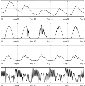
347
The different cross-correlation pairs are shown in Fig. 6, where each series shows the correlation between an input 348
candidate and the thermal power demand as a time shift is applied between the two signals. It is desirable that the selected 349
inputs show a high correlation with the target signal at the forecasting horizon, which is set to 1 hour in this case. As it can 350
be observed, the most strongly correlated input candidates when the offset between each pair is 1 hour are the external 351
temperature, the solar irradiance, the activity indicator and the bus return temperature. On the other hand, the bus impulsion 352
temperature and the bus temperature differential present low correlation with the target. Finally, it is noticeable that the 353
target shows a strong correlation with itself when a 1 hour offset is applied, therefore the current power demand value was 354
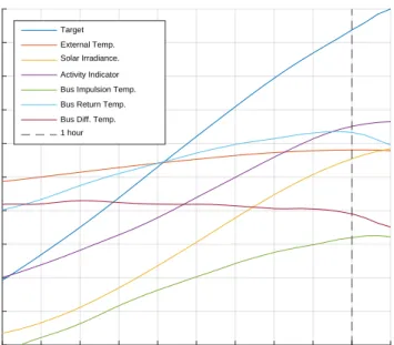
also considered as an input for the model. A sample of the preselected input variables is shown in Fig. 7. 355
Fig 6. Cross-correlation between each model input candidate and the forecasting target. -10 -9 -8 -7 -6 -5 -4 -3 -2 -1 0 Time [hours] 0 10 20 30 40 50 60 70 80 90 100 Cross-Correlation [%] Target External Temp. Solar Irradiance. Activity Indicator Bus Impulsion Temp. Bus Return Temp. Bus Diff. Temp. 1 hour
356
The study of the signal’s frequency components, shown in Fig. 8 as the frequency spectrum analysis, revealed the 357
magnitude of the signal’s dynamics. As it can be observed, the solar irradiation and the external temperature present rather 358
slower dynamics than the power demand, which is expected as they mostly follow a daily pattern. Instead, the activity 359
indicator presents significant dynamics up to sub-hour period frequencies, which is more aligned with those observed in the 360
power demand, as is the case of the bus return temperature, which presents even higher frequency components. Thus, the 361
inclusion of the activity indicator and the bus return temperature may help the model to better adapt to the power demand’s 362
dynamics, as these signals present more similar frequency components. 363
364
Additional empirical analyses carried out with the available signals, reveal that the use of both the external temperature 365
and the solar irradiance do not improve the modeling performance, as these two signals present correlation between them 366
and introduce redundant information into the model. As the external temperature presents a smoother behavior than the 367
solar irradiance, which has very steep peaks due to passing clouds, and a forecast of the external temperature is readily 368
available through a local weather service provider, but not for the case of the irradiance, the latter was discarded and only 369
the former was used. Regarding the current value of the target, it was noticed that it improved the forecasting accuracy 370
when included, as it provided a reference point to calculate the next values. Concerning the bus temperature signals, only 371
the return temperature was used, as it provides feedback about the state of the production/demand match. The bus 372
differential temperature was considered, even though it presented low correlation with the target, in an attempt to increase 373
Fig 7. Selected input variables during a period of 5 days in August.
Aug 08 Aug 09 Aug 10 Aug 11 Aug 12 Aug 13 0
0.5 1
External Temp.
Aug 08 Aug 09 Aug 10 Aug 11 Aug 12 Aug 13 0
0.5 1
Solar Irrad.
Aug 08 Aug 09 Aug 10 Aug 11 Aug 12 Aug 13 0
0.5 1
Activity Ind.
Aug 08 Aug 09 Aug 10 Aug 11 Aug 12 Aug 13 0
0.5 1
Bus Ret. Temp.
Fig 8. Frequency spectrum comparison between the power demand model input candidates and the power demand target signal.
0 0.5 1 1.5 2 2.5 3 Frequency [hours - 1] 0 0.01 0.02 Power 0 1 2 3 0 0.01 0.02 External Temp. 0 1 2 3 0 0.01 0.02 Activity Ind. 0 1 2 3 0 0.01 0.02 Solar Irrad. 0 1 2 3 0 0.01 0.02
the accuracy of the model during rapid changes, as the bus differential presents high dynamics. This helps the model 374
perform better in some cases, but overall introduces noise and is finally discarded. Finally, another considered variable is 375
the day of the week, which was included as it helps the ANFIS rule inference step to properly characterize the behavior of 376
the power demand during weekends. In summary, the study revealed that the most appropriate set of signals to characterize 377
the power demand of the building is: the external temperature, the activity indicator, the bus return temperature, the current 378
power demand value and the day of the week. 379
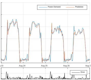
The result of the model training is shown in Fig. 9, where it can be observed that the model closely matches the target 380
on most of the signal, presenting low average error. However, there are also error peaks that occur when the target signal 381
presents the fastest dynamics, causing error spikes due to steep changes, but having very short duration. 382
383
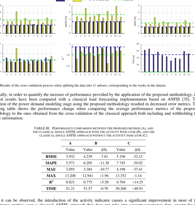
In order to validate the methodology and to evaluate its performance and generalization capabilities, a cross-validation 384
strategy was followed. The cross-validation implementation removes one week of data at a time from the dataset, builds a 385
model using the remaining data and validates the model against the removed subset. Thus an 11-fold cross-validation is 386
considered. The results of the cross-validation are shown in Fig. 10, where several performance indicators were calculated 387
when the model is applied over the training set and separately over the validation set. As it can be observed, the error 388
indicators are quite low, with the mean absolute error being the most compelling at an average value of 2% during training 389
and 3% during validation. The maximum error shows an average of 13%, which is acceptable due to the occasional rapid 390
changes observed in the signal, but reaches a value of 26% when week 3 is not present in the training set. In fact, the other 391
error indicators are also noticeably higher when week 3 is used as validation and is excluded from the training. This 392
observation indicates that week 3 presents a behavior that differs from the rest of the data, as the resulting model achieves 393
worse prediction performance when learning from the other cases. 394
Fig 9. Comparison between the power demand signal and a prediction obtained using the trained power demand model.
Aug 23 Aug 24 Aug 25 Aug 26 Aug 27 0 0.2 0.4 0.6 0.8 1
Power Demand Prediction
Aug 23 Aug 24 Aug 25 Aug 26 Aug 27 0
0.1 0.2
395
Finally, in order to quantify the increase of performance provided by the application of the proposed methodology, the 396
obtained results have been compared with a classical load forecasting implementation based on ANFIS [35]. The 397
evaluation of the power demand modeling stage using the proposed methodology resulted in decreased error metrics. The 398
following table shows the performance change when comparing the average performance metrics of the proposed 399
methodology to the ones obtained from the cross-validation of the classical approach both including and withholding the 400
activity information. 401
402
As it can be observed, the introduction of the activity indicator causes a significant improvement in most of the 403
performance metrics over a classical ANFIS approach that does not take into account occupancy data, except for the 404
training time, which is almost halved. This reduction in the duration of the training time is likely due to the reduction in the 405
size of the data and the loss of one dimension in the input space by not considering the activity indicator, which allowed the 406
modeling to speed up convergence at the cost of increased error. Additionally, the integration of the occupancy forecasting 407
in the proposed methodology in order to provide more updated activity values helped to further increase the performance 408
metrics over a classical approach that used the activity indicator. 409
5.
Conclusions
410
A short-term activity-aware thermal power demand forecasting methodology is studied in this paper, aligned with the 411
state of the art on load forecasting in buildings for energy management applications. The proposed methodology consists in 412
a hybrid modeling process where a dedicated recurrent neural network learns the dynamics present in an activity indicator 413
developed for this study, and an adaptive neuro-fuzzy inference system correlates activity predictions obtained in this 414
manner with the outdoor temperature and the bus return temperature in order to characterize the thermal power demand of 415
the building’s HVAC system. 416
The integration of the activity assessment into the modeling process, through the definition of an indicator that reflects 417
the occupancy state of the whole building, has been shown to increase the accuracy of the power demand forecasting. The 418
error metrics are significantly decreased when the activity is used as an additional input for the power demand forecasting, 419
but they are further diminished when the neural network is included as a dedicated means to learn the activity’s dynamics, 420
providing an estimation of the use that the building shall receive in the following hour. To this end, the implementation of 421
Fig 10. Results of the cross-validation process when splitting the data into 11 subsets, corresponding to the weeks in the dataset.
1 2 3 4 5 6 7 8 9 10 11 0 2 4 6 8 RMSE [%] 1 2 3 4 5 6 7 8 9 10 11 0 2 4 6 8 MAPE [%] 1 2 3 4 5 6 7 8 9 10 11 0 2 4 6 8 MAE [%] 1 2 3 4 5 6 7 8 9 10 11 0 10 20 30 MAX [%] 1 2 3 4 5 6 7 8 9 10 11 0.6 0.8 1 R 2 1 2 3 4 5 6 7 8 9 10 11 0 20 40 60 80 Time [s]
Train Test mean(Train) mean(Test)
TABLEIII. PERFORMANCE COMPARISON BETWEEN THE PROPOSED METHOD (A), AND
THE CLASSICAL SINGLE ANFIS APPROACH WITH THE ACTIVITY INDICATOR (B), AND THE
CLASSICAL SINGLE ANFIS APPROACH WITHOUT THE ACTIVITY INDICATOR (C).
A B C
Value Value ∆% Value ∆%
RMSE 3.932 4.239 -7.81 5.196 -32.15 MAPE 5.571 6.205 -11.38 7.745 -39.02 MAE 3.055 3.384 -10.77 4.198 -37.41 MAX 13.200 12.941 +1.96 13.352 -1.14 R2 0.821 0.775 +5.58 0.704 +14.25 TIME 51.21 51.57 -0.70 30.260 +40.91
the activity modeling with a recurrent neural network is validated as suitable approach in order to consider the temporal 422
patterns of the building’s activity, as the proposed activity modeling process exhibits an important performance increase 423
compared with state-of-the-art approaches, achieving a mean absolute error below 10%. 424
The proposed thermal power demand estimation procedure allows the modelling of the total power being drawn by the 425
consumption endpoints in the building, instead of modelling the consumption of the entire installation as is done in most 426
related studies. The estimation is achieved by means of an energy meter that monitors the aggregate output of the 427
production stage equipment and the simulation of the bus capacity in order to calculate the difference. The main benefit of 428
this change is to allow the decoupling of the effect of the capacity of the distribution bus and the effect of the management 429
strategy followed by the HVAC energy production equipment. Therefore, future studies may build on this methodology for 430
implementing production management strategies that optimize the operation of the equipment according to the forecasted 431
power demand in order to increase the energy efficiency. 432
A study of the available input candidates for implementing the power demand model was carried out in order to obtain 433
a set of variables that allows the accurate modelling of the target signal. This study helped identify the set that achieves the 434
best results: the current power demand, the activity indicator, the external temperature, the bus return temperature and the 435
day of the week. The developed methodology can be generalized to other cases, extending its applicability. 436
Besides increased accuracy, the proposed methodology presents other advantages, such as the possibility of using 437
separate datasets of potentially different sizes for the activity indicator model and for the power demand model, which 438
allowed the selection of representative datasets for each case. Additionally, this decoupling allowed the separation of 439
concerns, promoting the specialization during the selection of the best modeling algorithm for each signal and the 440
independent tuning of the configuration of each model, including the use of different inputs and dynamics to match each 441
target signal’s behavior. The proposed structure also decouples the model tuning process, allowing to update a model 442
independently of the other when necessary, since the activity model may need to be updated more often due to the 443
changing behavior of the activity of the building. 444
References
445[1] D. Wijayasekara, O. Linda, M. Manic, and C. Rieger, "Mining Building Energy Management System Data Using Fuzzy Anomaly Detection
446
and Linguistic Descriptions," Industrial Informatics, IEEE Transactions on, vol. 10, no. 3, pp. 1829-1840, 2014.
447
[2] I. Lampropoulos, W. L. Kling, P. F. Ribeiro, and J. van den Berg, "History of demand side management and classification of demand
448
response control schemes," in Power and Energy Society General Meeting (PES), 2013 IEEE, 2013, pp. 1-5.
449
[3] K. O. Aduda, T. Labeodan, W. Zeiler, G. Boxem, and Y. Zhao, "Demand side flexibility: Potentials and building performance implications,"
450
Sustainable Cities and Society, vol. 22, pp. 146-163, 4// 2016.
451
[4] G. Graditi et al., "Innovative control logics for a rational utilization of electric loads and air-conditioning systems in a residential building,"
452
Energy and Buildings, vol. 102, pp. 1-17, 2015/09/01/ 2015.
453
[5] I. Sartori, A. Napolitano, and K. Voss, "Net zero energy buildings: A consistent definition framework," Energy and Buildings, vol. 48, pp.
454
220-232, 5// 2012.
455
[6] S. Biao, P. B. Luh, J. Qing-Shan, J. Ziyan, W. Fulin, and S. Chen, "Building Energy Management: Integrated Control of Active and Passive
456
Heating, Cooling, Lighting, Shading, and Ventilation Systems," Automation Science and Engineering, IEEE Transactions on, vol. 10, no. 3,
457
pp. 588-602, 2013.
458
[7] A. Costa, M. M. Keane, J. I. Torrens, and E. Corry, "Building operation and energy performance: Monitoring, analysis and optimization
459
toolkit," Applied Energy, vol. 101, no. 0, pp. 310-316, 2013.
460
[8] A. H. Neto and F. A. S. Fiorelli, "Comparison between detailed model simulation and artificial neural network for forecasting building
461
energy consumption," Energy and Buildings, vol. 40, no. 12, pp. 2169-2176, // 2008.
462
[9] J. Grant, M. Eltoukhy, and S. Asfour, "Short-Term Electrical Peak Demand Forecasting in a Large Government Building Using Artificial
463
Neural Networks," Energies, vol. 7, no. 4, p. 1935, 2014.
464
[10] G. Qiang, T. Zhe, D. Yan, and Z. Neng, "An improved office building cooling load prediction model based on multivariable linear
465
regression," Energy and Buildings, vol. 107, pp. 445-455, 11/15/ 2015.
466
[11] Q. Zhou, S. Wang, X. Xu, and F. Xiao, "A grey-box model of next-day building thermal load prediction for energy-efficient control,"
467
International Journal of Energy Research, vol. 32, no. 15, pp. 1418-1431, 2008.
468
[12] Z. Liu, H. Tan, D. Luo, G. Yu, J. Li, and Z. Li, "Optimal chiller sequencing control in an office building considering the variation of chiller
469
maximum cooling capacity," Energy and Buildings, vol. 140, pp. 430-442, 2017/04/01/ 2017.
470
[13] Y.-C. Chang, "Application of Hopfield Neural Network to the optimal chilled water supply temperature calculation of air-conditioning
471
systems for saving energy," International Journal of Thermal Sciences, vol. 48, no. 8, pp. 1649-1657, 2009/08/01/ 2009.
472
[14] B. Yildiz, J. I. Bilbao, and A. B. Sproul, "A review and analysis of regression and machine learning models on commercial building
473
electricity load forecasting," Renewable and Sustainable Energy Reviews, vol. 73, pp. 1104-1122, 6// 2017.
474
[15] T. Hong and S. Fan, "Probabilistic electric load forecasting: A tutorial review," International Journal of Forecasting, vol. 32, no. 3, pp.
914-475
938, 7// 2016.
476
[16] C. Kuster, Y. Rezgui, and M. Mourshed, "Electrical load forecasting models: A critical systematic review," Sustainable Cities and Society,
477
vol. 35, pp. 257-270, 2017/11/01/ 2017.
478
[17] S. Ferlito, G. Adinolfi, and G. Graditi, "Comparative analysis of data-driven methods online and offline trained to the forecasting of
grid-479
connected photovoltaic plant production," Applied Energy, vol. 205, pp. 116-129, 2017/11/01/ 2017.
480
[18] M. Peña, F. Biscarri, J. I. Guerrero, I. Monedero, and C. León, "Rule-based system to detect energy efficiency anomalies in smart buildings,
481
a data mining approach," Expert Systems with Applications, vol. 56, pp. 242-255, 9/1/ 2016.
482
[19] T. Hong, S. C. Taylor-Lange, S. D’Oca, D. Yan, and S. P. Corgnati, "Advances in research and applications of energy-related occupant
483
behavior in buildings," Energy and Buildings, vol. 116, pp. 694-702, 3/15/ 2016.
484
[20] B. Chenari, J. Dias Carrilho, and M. Gameiro da Silva, "Towards sustainable, energy-efficient and healthy ventilation strategies in buildings:
485
A review," Renewable and Sustainable Energy Reviews, vol. 59, pp. 1426-1447, 6// 2016.
486
[21] M. Jia, R. S. Srinivasan, and A. A. Raheem, "From occupancy to occupant behavior: An analytical survey of data acquisition technologies,
487
modeling methodologies and simulation coupling mechanisms for building energy efficiency," Renewable and Sustainable Energy Reviews,
488
vol. 68, Part 1, pp. 525-540, 2// 2017.
[22] W. Zeyu and R. S. Srinivasan, "A review of artificial intelligence based building energy prediction with a focus on ensemble prediction
490
models," in 2015 Winter Simulation Conference (WSC), 2015, pp. 3438-3448.
491
[23] J. Massana, C. Pous, L. Burgas, J. Melendez, and J. Colomer, "Short-term load forecasting in a non-residential building contrasting models
492
and attributes," Energy and Buildings, vol. 92, pp. 322-330, 4/1/ 2015.
493
[24] J. Massana, C. Pous, L. Burgas, J. Melendez, and J. Colomer, "Short-term load forecasting for non-residential buildings contrasting artificial
494
occupancy attributes," Energy and Buildings, vol. 130, pp. 519-531, 10/15/ 2016.
495
[25] Y. S. Lee and A. M. Malkawi, "Simulating multiple occupant behaviors in buildings: An agent-based modeling approach," Energy and
496
Buildings, vol. 69, pp. 407-416, 2014/02/01/ 2014.
497
[26] J. Virote and R. Neves-Silva, "Stochastic models for building energy prediction based on occupant behavior assessment," Energy and
498
Buildings, vol. 53, pp. 183-193, 2012/10/01/ 2012.
499
[27] Z. Chen, J. Xu, and Y. C. Soh, "Modeling regular occupancy in commercial buildings using stochastic models," Energy and Buildings, vol.
500
103, pp. 216-223, 9/15/ 2015.
501
[28] Z. Yang and B. Becerik-Gerber, "The coupled effects of personalized occupancy profile based HVAC schedules and room reassignment on
502
building energy use," Energy and Buildings, vol. 78, pp. 113-122, 8// 2014.
503
[29] Y. T. Chae, R. Horesh, Y. Hwang, and Y. M. Lee, "Artificial neural network model for forecasting sub-hourly electricity usage in
504
commercial buildings," Energy and Buildings, vol. 111, pp. 184-194, 1/1/ 2016.
505
[30] J. Zhao, B. Lasternas, K. P. Lam, R. Yun, and V. Loftness, "Occupant behavior and schedule modeling for building energy simulation
506
through office appliance power consumption data mining," Energy and Buildings, vol. 82, pp. 341-355, 10// 2014.
507
[31] Ö. F. Ertugrul, "Forecasting electricity load by a novel recurrent extreme learning machines approach," International Journal of Electrical
508
Power & Energy Systems, vol. 78, pp. 429-435, 2016/06/01/ 2016.
509
[32] A. Laouafi, M. Mordjaoui, S. Haddad, T. E. Boukelia, and A. Ganouche, "Online electricity demand forecasting based on an effective
510
forecast combination methodology," Electric Power Systems Research, vol. 148, pp. 35-47, 7// 2017.
511
[33] S. Barak and S. S. Sadegh, "Forecasting energy consumption using ensemble ARIMA–ANFIS hybrid algorithm," International Journal of
512
Electrical Power & Energy Systems, vol. 82, pp. 92-104, 2016/11/01/ 2016.
513
[34] C. Deb, F. Zhang, J. Yang, S. E. Lee, and K. W. Shah, "A review on time series forecasting techniques for building energy consumption,"
514
Renewable and Sustainable Energy Reviews, vol. 74, pp. 902-924, 7// 2017.
515
[35] E. Sala, K. Kampouropoulos, F. Giacometto, and L. Romeral, "Smart multi-model approach based on adaptive Neuro-Fuzzy Inference
516
Systems and Genetic Algorithms," in Industrial Electronics Society, IECON 2014 - 40th Annual Conference of the IEEE, 2014, pp. 288-294.
517 518