Hierarchical Bayes variable selection and microarray experiments

(1)

www.elsevier.com/locate/jmva

Hierarchical Bayes variable selection and microarray

experiments

David J. Nott

a,b,∗

_{, Zeming Yu}

a

_{, Eva Chan}

b

_{, Chris Cotsapas}

b

_,

Mark J. Cowley

b

, Jeremy Pulvers

b

, Rohan Williams

b

, Peter Little

b

a_{Department of Statistics, University of New South Wales, Sydney 2052, Australia}

b_{School of Biotechnology and Biomolecular Sciences, University of New South Wales, Sydney 2052, Australia} Received 12 July 2005

Available online 21 November 2006

Abstract

Hierarchical and empirical Bayes approaches to inference are attractive for data arising from microarray gene expression studies because of their ability to borrow strength across genes in making inferences. Here we focus on the simplest case where we have data from replicated two colour arrays which compare two samples and where we wish to decide which genes are differentially expressed and obtain estimates of operating char-acteristics such as false discovery rates. The purpose of this paper is to examine the frequentist performance of Bayesian variable selection approaches to this problem for different prior specifications and to examine the effect on inference of commonly used empirical Bayes approximations to hierarchical Bayes procedures. The paper makes three main contributions. First, we describe how the log odds of differential expression can usually be computed analytically in the case where a double tailed exponential prior is used for gene effects rather than a normal prior, which gives an alternative to the commonly usedB-statistic for ranking genes in simple comparative experiments. The second contribution of the paper is to compare empirical Bayes pro-cedures for detecting differential expression with hierarchical Bayes methods which account for uncertainty in prior hyperparameters to examine how much is lost in using the commonly employed empirical Bayes approximations. Third, we describe an efficient MCMC scheme for carrying out the computations required for the hierarchical Bayes procedures. Comparisons are made via simulation studies where the simulated data are obtained by fitting models to some real microarray data sets. The results have implications for analysis of microarray data using parametric hierarchical and empirical Bayes methods for more complex experimental designs: generally we find that the empirical Bayes methods work well, which supports their use in the

∗_{Corresponding author. Department of Statistics, University of New South Wales, Sydney 2052, Australia.} Fax: +61 2 9385 7123.

E-mail address:[email protected](D.J. Nott).

(2)

analysis of more complex experiments when a full hierarchical Bayes analysis would impose heavy compu-tational demands.

Keywords:Bayesian model selection; Hierarchical Bayes; Microarrays

1. Introduction

Empirical Bayes methods are attractive for inference for microarray experiments because of their ability to borrow strength across genes for making inferences. In this paper we consider the simple case where we have replicated data from two colour microarrays for a comparison of two samples and where our interest lies in detecting differentially expressed genes and estimating operating characteristics such as false discovery rates. The problem here can be approached by variable selection methods for linear models, and in this paper we consider empirical and hierarchical Bayes approaches. For the case of a constant known variance parameter an insightful discussion of empirical Bayes variable selection methods for linear models was given by George and Foster[9]. They consider a binomial prior for the number of active terms and a normal prior for the coefﬁcients of active terms and showed that for certain choices of the hyperparameters in their priors the ranking of models according to posterior probability agrees with ranking via various classical model selection criteria such as AIC [1], BIC [20] and RIC [8]. Estimating the hyperparameters results in a procedure able to adaptively approximate the best of these criteria. If prior hyperparameters are estimated conditional on the model, an explicit expression can be given for the empirical Bayes criterion which is somewhat reminiscent of false discovery rate controlling procedures [3] in that the penalty for an additional term added decreases with the number of effects already discovered.

These observations suggest that empirical Bayes variable selection procedures represent a promising approach for the analysis of data from microarray experiments. For microarray data, parametric empirical Bayes model selection approaches have been considered by Baldi and Long [2], Kendziorski et al. [13], Lönnstedt and Speed [16], Newton and Kendziorski [18], Newton et al. [19] and Smyth [21]. See also Broët et al. [4], Ibrahim et al. [11], Kauermann and Eilers [12] and Lönnstedt et al. [16]. Our approach is closest to that of Lönnstedt and Speed [17] who also considered replicated microarrays for simple comparative experiments. They consider a normal prior for effects of genes which are differentially expressed and an inverse gamma prior for gene variances. These priors allow an explicit expression for the log odds of differential expression to be derived (the so-calledB-statistic) after suitable values for the prior hyperparameters have been obtained.

The present paper makes three main contributions. First, we consider an exponential power prior for the effects of genes which are differentially expressed and in the special case of a double tailed exponential prior are able to obtain an expression for the log odds of differential expres-sion similar to theB-statistic of Lönnstedt and Speed [17]. The double tailed exponential prior is more heavy tailed than the normal, which may be appropriate for many real data sets, and is related to the lasso of Tibshirani [22]. The second contribution of our paper is to compare empirical Bayes approaches to detection of differential expression with hierarchical Bayes ap-proaches which account for uncertainty in prior hyperparameters. One practical advantage of the

(3)

hierarchical Bayes approach over empirical Bayes approaches is that in the empirical Bayes meth-ods point estimates of hyperparameters such as the prior probability of differential expression may be on the boundary of the parameter space, resulting in all genes having posterior probability of differential expression of zero or one. Accounting for hyperparameter uncertainty in the hier-archical Bayes approach may result in more realistic inferences both in this situation and quite generally. Examining hierarchical Bayes procedures enables us to examine how much is lost via the commonly used empirical Bayes approximations, which has lessons for the analysis of data from more complex experimental designs: it is interesting to know whether the computational overhead of a full hierarchical Bayes analysis is worth the effort. In general, we ﬁnd that the empirical Bayes methods work well which supports their use in statistical practice. In addition, the comparison of results for different priors allows us to investigate questions of whether the results of parametric empirical Bayes analyses are sensitive to the form of the prior. This also has implications for the analysis of data from more complex experiments. Our third contribution is to describe an efﬁcient MCMC algorithm for implementing the computations required for the hierarchical Bayes approaches.

We do not consider in this paper the problem of normalization of microarray data, where sys-tematic sources of variation unrelated to genetic effects of interest are removed. For instance, it is well known as the raw log expression ratios in microarray experiments vary with the spot intensity. Usually normalization is done prior to and independent of any assessment of significance of gene effects which is what we do in the examples considered later. This ignores the uncertainty about the normalization step in subsequent inference for gene effects. Recently there have been efforts to integrate normalization and assessments of significance: for a discussion of these approaches and of the problem of array specific intensity location and scale effects see Lewin et al.[14], Fan et al. [7] and Huang et al. [10].

The structure of the paper is as follows. In the next section we discuss empirical Bayes variable selection for microarrays and the prior speciﬁcations we consider. We also describe how to calcu-late the log odds of differential expression for a double tailed exponential prior on gene effects. In Section 3 we consider hierarchical Bayes approaches to the problem and describe our MCMC scheme for carrying out the computations required for inference in this case. In Section 4 we compare the performance of different priors and the hierarchical and empirical Bayes procedures in some simulation studies. Finally, Section 5 gives some discussion and conclusions.

2. Empirical Bayes variable selection for microarrays

2.1. Model and prior distributions

LetMgj,g = 1, . . . , G,j = 1, . . . , n, be data from a replicated microarray experiment to compare gene expression under two experimental conditions, wheregindexes different genes andjindexes different arrays (replicates). For two colour microarrays the data come in the form of normalized log ratios of expression level measurements under the two conditions. We consider the model

Mgj =g+gj,

where_g is a gene speciﬁc mean andgj ∼ N (0,2g)where2g is a gene speciﬁc variance.

The errorsgj are independent and ifg =0 then genegis not differentially expressed under

the two experimental conditions. In what follows, instead of interpreting differential expression as meaning_g = 0 we consider that a gene is differentially expressed if|_g| > k and not

(4)

differentially expressed if|g|kwherekis some cutoff. In general,kmight be chosen depending

on the purpose of the experiment and possible confounding sources of variation. It is often found in microarray data that there are many small effects, and the genes most likely to be interesting for further examination and experimentation are those with large effects. Hence our framework considers differential expression deﬁned in this way, where of course we can setk=0 if the size of the effect is not considered informative about which genes are of greatest biological interest.

We consider various priors ongand2g for doing Bayesian inference and our main interest

lies in the meansg. We summarize information aboutgthrough the quantity

B(k)=logPr(|g|> k|M)

Pr(|_g|k|M), (1)

where we have writtenPr(A|M)for the posterior probability of eventAgiven the dataM and

kis the cutoff parameter described above. Lönnstedt and Speed[17] consideredk = 0 and a prior on_gwhich allows_gto be exactly zero. For their prior on_gand a certain prior on2_g they were able to calculateB(0)explicitly, which they called theB-statistic. TheB-statistic has been generalized by Smyth [21] to a linear models framework. Both Lönnstedt and Speed [16] and Smyth [21] suggest that theB-statistic is of more interest as a way of ranking genes rather than for formal inferences. The attractiveness of Bayesian methods for ranking or inference lies in the ability to borrow strength across genes through the use of hierarchical priors on gene level parameters.

The purpose of this paper is to compare the performance of hierarchical and empirical Bayes procedures for detecting differential expression for different prior speciﬁcations ong. We are also interested in model based estimates of false discovery rates or other operating character-istics following a so-called direct posterior probability approach to inference [19]. Suppose we have declared a certain setD ⊂ {1, . . . , G}of the genes as differentially expressed (by geneg

being differentially expressed we mean|g|k). The posterior expected number of genes not differentially expressed among those declared differentially expressed is

g∈D

Pr(|_g|k|M)

and dividing this by#D(where#Adenotes the size of setA) gives a model based estimate of the false discovery rate.

Following the prior speciﬁcation used in Smyth[21], we consider a prior speciﬁcation on the gene variances2_gwhich is inverse gamma,

2 g∼I G n0 2 , n0s₀2 2 ,

wheren0ands02are hyperparameters. The prior above can be thought of as information on2gof

a prior estimates₀2onn0degrees of freedom. It remains to specify a prior on the meansg. We

havep=Pr(g=0)and given thatg =0,ghas an exponential power prior

p(_g|2_g,_g=0)= 1 2(2c2 g) 1 b₁+1 b exp −|g|b 2c2 g ,

wherebandcare hyperparameters. Settingb =2 gives a normal prior (similar to[17,21]) and settingb = 1 gives a double tailed exponential prior. Note that there is a certain dependence

(5)

betweengand2gin the prior here. In some cases having the scale of the prior ongdependent

on2_gmay be natural (for instance, if prior information aboutgwere somehow based on a ﬁxed

number of past observations) but the form of prior adopted here is primarily chosen for analytical convenience.

2.2. Log odds of differential expression

To evaluate (1), observe that

Pr(|_g|> k|M)=Pr(|_g|> k, _g=0|M)

=Pr(_g=0|M)Pr(|_g|> k|M,_g =0) (2) and of coursePr(|g|k|M)=1−Pr(|g|> k|M). We ﬁnd an expression forPr(g=0|M)

and for the posterior distribution ofggiveng =0 which allows (2) to be calculated.

We writeMg=(Mg1, . . . , Mgng)

T_{for the data for gene}_g_{. We allow the number of observations} to vary for each gene to allow for missing data. Now,

Pr(_g=0|M)=Pr(_g=0|Mg)

= p p(Mg|g =0)

p p(Mg|g =0)+(1−p) p(Mg|g=0) ,

wherep(Mg|g =0)is the marginal likelihood ofMggiveng =0 andp(Mg|g =0)is the marginal likelihood ofMggiveng =0. For convenience we have suppressed dependence on the prior hyperparameters in our notation for the marginal likelihoods. We give expressions for the marginal likelihoods now, which are derived in the Appendix.

First, p(Mg|g=0)= −ng 2 (n₀s2 0) n₀ 2 n0+ng 2 n0 2 ⎛ ⎝n0s02+ j M_gj2 ⎞ ⎠ −n₀+ng 2 .

In the caseb=2 (a normal prior for gene effects) we obtain

p(Mg|g=0)= −ng2 _(n₀_s2 0) n0 2 n0+ng 2 (cng+1) 1 2n0 2 ⎛ ⎝n0s02+ j M_gj2 − cng 1+cng ngM¯g2 ⎞ ⎠ −n0+ng 2

which is the expression in Lönnstedt and Speed[17] and Smyth [21]. In the caseb=1 (a double tailed exponential prior for gene effects) we obtain

p(Mg|g=0)= G(_g,1, c, n0, s02) dg =K(1, c, n0, s02) ⎛ ⎝n0s20+ |g| c + j (Mgj −g)2 ⎞ ⎠ −n0+ng+2 2 d_g, where K(1, c, n0, s02)= −ng2 _(n₀_s2 0) n0 2 n0+ng+2 2 2cn0 2 .

(6)

We can write the integral asI1+I2where I1= _∞ 0 ⎛ ⎝n0s02+ g c + j (Mgj −g)2 ⎞ ⎠ −n0+ng+2 2 d_g and I2= 0 −∞ ⎛ ⎝n0s02− g c + j (Mgj −g)2 ⎞ ⎠ −n0+ng+2 2 d_g.

WriteM¯g+= ¯Mg+1/(2cng),M¯g−= ¯Mg−1/(2cng),T ∼t(,2)to denote that the random

variableThas at-distribution withdegrees of freedom, mean and scale parameter2, and

B(·,·)for the beta function. If

n0s02+ j M_gj2 −ngM¯g2−>0 and n0s02+ j M_gj2 −ngM¯g2+>0 (3)

we can show (see the Appendix)

I1=n− 1 2 g B 1 2, n0+ng+1 2 ⎛ ⎝n0s02+ j M_gj2 −ngM¯g2− ⎞ ⎠ −n₀+ng+1 2 Pr(T1>0), where T1∼tn0+ng+1 ¯ Mg−, n0s02+ jMgj2 −ngM¯ 2 g− (n0+ng+1)ng and I2=n− 1 2 g B 1 2, n0+ng+1 2 ⎛ ⎝n0s02+ j M_gj2 −ngM¯g2+ ⎞ ⎠ −n0+ng+1 2 Pr(T2<0), where T2∼tn0+ng+1 ¯ Mg+, n0s₀2+_jM_gj2 −ngM¯g2+ (n0+ng+1)ng .

So if (3) holds we can explicitly write the marginal likelihood in terms of the distribution function of certainTrandom variables. While condition (3) is usually satisﬁed, if it does not thenp(Mg|g= 0)cannot be written in terms of distribution functions ofTrandom variables as above, but the required integrations can be done using some numerical integration method. Note that for the double exponential prior if we were to ﬁxp=1 (no variable selection) and if we estimategas the posterior mode, then many of the estimates would still be exactly zero. In fact, the posterior mode for_gis sign(M¯g) | ¯Mg| − 1 2cng + ,

(7)

wherez₊ = max(0, z)is the positive part of z and sign(M¯g)is 1 if M¯g is positive and −1

otherwise. The use of the double tailed exponential prior is related to the lasso of Tibshirani[22]. So far we have described the evaluation ofPr(_g =0|M). We also need the posterior distri-bution ofggiveng=0 in order to calculate (2). Whenb=2 (a normal prior) the distribution ofg|g=0, Mis at-density (see the Appendix),

tn0+ng cng 1+cng ¯ Mg, cng 1+cng n0s20+ jMgj2 − cng 1+cngngM¯ 2 g ng(n0+ng) . (4)

So in this case we can easily calculate (2). In the case ofb =1 (the double tailed exponential prior) p(_g|Mg,g =0) ∝ −ng 2 (n₀s2 0) n₀ 2 n0+ng+2 2 2cn0 2 × ⎛ ⎝n0s02+ |g| c + j (Mgj−g) 2 ⎞ ⎠ −n0+ng+2 2 .

If (3) holds, this density is a mixture of two constrainedt-densities. WithI1,I2,T1andT2deﬁned as before, the density of_g|_g=0, Mis the density of a random variableTwhere

T =

Z1 with probabilityI1/(I1+I2),

Z2 otherwise,

whereZ1=T1|T1>0 andZ2=T2|T20. Hence the required probability in (2) can be written in terms of distribution functions of certaint random variables if (3) holds, and the required probability can be evaluated numerically from the above expression for the unnormalized density otherwise. It is interesting to examine the mean and scale parameters forT1,T2and those in the distribution ofg|g = 0, M in the normal case—this shows the different kinds of shrinkage induced by the two different priors.

2.3. Estimation of hyperparameters

In our prior distribution for the parameters(_g,2_g),g=1, . . . , G, there are hyperparameters

(n0, s02, p, c, b). Here we consider an empirical Bayes approach where we estimate these param-eters from the data, with the exception of the parameterbwhich we fix at eitherb=1 orb=2 (the double tailed exponential and normal priors, respectively, where some of the calculations can be performed analytically). We do not estimatebsince as noted by Smyth [21] estimating many parameters in the prior ong|g =0 may be difficult since only differentially expressed genes contribute (perhaps only a small number) and there is an uncertainty about which genes are differentially expressed. Also, it is only in the case ofb =1 and 2 that substantial analytic simplification is possible which allows convenient computations. For the estimation ofn0ands₀2 we use the procedure outlined by Smyth [21]. Smyth [21] observes thatn0ands₀2can be very precisely estimated because all genes contribute to the estimation of these parameters. The only remaining parameters to be estimated arepandc, which we estimate by maximum likelihood with

(8)

n0ands02as they appear in the prior ong for differentially expressed genes. The log marginal

likelihood here (where we suppress dependence onb,n0ands₀2in the notation) is

logp(M|p, c)=

g

logp(Mg|p, c),

where

p(Mg|p, c)=(1−p) p(Mg|g=0)+p p(Mg|g=0).

Calculation of the marginal likelihoods in this expression was discussed in Section 2.2. The choice betweenb=1 and 2 in applications can also be based on maximized marginal likelihoods (this is equivalent to the use of BIC applied with the marginal likelihood integrating out random effects, since the number of parameters is the same in the two models). It is often found that point estimates ofpcan be on the boundary (that is, 0 or 1) which can result in the posterior probabilities of differential expression for all genes being zero or one. In empirical Bayes variable selection for linear models George and Foster [9] observe a similar phenomenon and note that since mixture priors like the one considered here do both variable selection (through the parameter p) and shrinkage (through the parameter c) then when there are many small effects the model may effectively give up on doing model selection and attempt to obtain good estimates of the means

g purely by doing shrinkage instead. The instability of estimation ofpandccaused Lönnstedt and Speed [16] to abandon the idea of estimating both these parameters. Instead, they ﬁxpand observe that the value ofpdoes not change the ranking of genes according toB(0)for ﬁxed values of the other hyperparameters. In general, it is inadvisable to interpret the parameterpas being the proportion of genes differentially expressed. Rather, we should think of the prior on theg’s with a point mass at zero as being a convenient and parsimonious approximation to a more continuous mixture prior with a low variance and high variance component. The problems associated with obtaining point estimates and ignoring uncertainty about prior hyperparameters by “plugging in” are avoided in the hierarchical Bayes approaches discussed next, where we consider posterior probabilities of differential expression obtained by averaging over the posterior distribution onp

andc.

3. Hierarchical Bayesian procedures

In this section we extend the analysis of Section 2 to the consideration of hierarchical Bayes procedures which attempt to account for uncertainty in the hyperparameterspandc. We estimate or ﬁxn0,s₀2andbin the same way as in Section 2 (as noted there,n0ands02can be very precisely estimated so there is not too much loss in ignoring uncertainty about these parameters). In our hierarchical Bayes approach we specify priors onpandcas follows. Forp, we use a uniform prior on the range[0,1]. Forc, we use a uniform prior on the range[0.01,100]. To get some

intuition for this choice observe that for the case of a normal priorb=2, the prior ong|g=0 can be considered equivalent to the information obtained from observing 1/cobservations at 0 so that our hyperprior oncallows priors on_g varying from fairly noninformative to informative. It only remains to describe our computational approach for calculating (1) taking into account our uncertainty about p andc. We use Markov chain Monte Carlo (MCMC) methods for the calculation of the posterior probabilityPr(|_g|> k|M)and the odds (1). For an introduction to MCMC methods see Liu [15].

(9)

Our sampling scheme generates dependent samples from the joint posterior distribution forp

andcwith all other parameters integrated out. We construct a Markov chain

C=

(p(j ), c(j )), j1

which has the posterior distributionp(p, c|M)as its stationary distribution. Then after choosing some initial values(p(1), c(1))arbitrarily and simulating the chainC for a long time (B +S

iterations say) and discarding the ﬁrstB iterations as a “burn in” sequence not typical of the stationary distribution then we obtain an approximate dependent sample from the posterior. We can estimatePr(|_g|> k|M)by 1 S B+S j=B+1 Pr(|_g|> k|M, p(j ), c(j )).

Calculation ofPr(|_g| > k|M, p(j ), c(j ))proceeds as for the empirical Bayes approaches of Section 2 ﬁxing(p, c)at(p(j ), c(j )). Our MCMC sampling scheme is described below.

At stepjfor the chainCwe generate(p(j+1), c(j+1))from(p(j ), c(j ))as follows.

1. Generate a proposal value(p∗, c∗)for(p(j+1), c(j+1))from a proposal distributionq(p, c,| p(j ), c(j ))(discussed further below).

2. Accept(p(j+1), c(j+1))=(p∗, c∗)with probability min{1,}, where

= p(M|p∗, c∗) p(M|p(j )_{, c}(j )₎ q(p(j ), c(j )|p∗, c∗) q(p∗, c∗|p(j )_{, c}(j )₎I (p ∗_{∈ [}₀_,₁_]_{, c}∗_{∈ [}₀_.₀₁_,₁₀₀_]_). Otherwise,(p(j+1), c(j+1))=(p(j ), c(j )).

To complete the speciﬁcation of our sampling scheme we need to describe the proposal distribution in the above algorithm. Forq(p, c|p(j ), c(j ))we simply use a random walk proposal, a uniform distribution on a rectangle centered at(p(j ), c(j )),[p(j )−hp, p(j )+hp] × [c(j )−hc, c(j )+hc]

where in the examples later we sethp = hc = 0.05. In the simulation studies discussed next

it was observed that the posterior mean estimates of the parametersp andcobtained from the MCMC iterates were generally similar to the marginal maximum likelihood estimates employed in our empirical Bayes approach.

4. Simulation studies

We compare the performance of the procedures of Sections 2 and 3 in simulation studies. Four procedures are compared: the empirical Bayes procedures with normal or double tailed exponential priors and the hierarchical Bayes procedure with normal or double tailed exponential priors. We have taken two real data sets and estimated hyperparameters for both priors following the empirical Bayes methodology of Section 2. Then 50 simulated data sets were generated for each of the two sets of hyperparameters whereg and2g are simulated from the prior and all variable selection procedures are applied.

We consider the statisticB(k) fork = log 1.25,log 1.5,log 2. For each method and a given cutoffk, a gene is called differentially expressed ifB(k) >0 (that is, ifPr(|_g|> k|M) >0.5). The threshold on the posterior probability of 0.5 is appropriate if false positive and false negative results are equally serious, but a different threshold can be used if this is not the case. For each

(10)

method we calculate the false discovery rate (FDR) which is the proportion of genes wrongly declared differentially expressed, defined to be zero if no genes are declared differentially ex-pressed. We also calculate a model based estimate of the false discovery rate (FDR) as described in Section2.1 as the posterior expected proportion of genes not differentially expressed among those declared differentially expressed. Similarly, we calculate the false negative rate (FNR) which is the proportion of genes which are differentially expressed among those which are not declared differentially expressed, defined to be zero if all genes are declared differentially expressed. We can also calculate a model based estimate of the false negative rate (FNR) for each method as the posterior expected proportion of genes differentially expressed among those not declared dif-ferentially expressed. We also report the number actually difdif-ferentially expressed at each cutoff (NDE), the number wrongly declared differentially expressed or number of false positives (NFP) and the number wrongly declared not differentially expressed or false negatives (NFN). Values reported in the tables for FDR, FDR–FDR, FNR, FNR– FNR and NDE are average values, averaging over the replicates in the simulation study for each case. The values NFP and NFN are derived as NFP=NDE×FDR and NFN =(G-NDE)×FNR, respectively. We stress once more that our definitions of differential expression, of a false discovery and of a false negative depend onkso that it is very natural and expected that NDE, FDR and FNR will vary a lot between differentk. Also, when comparing FDRs for the different priors, it must also be kept in mind that the FDRs are for different numbers of genes declared differentially expressed. In the results for the hierarchical analyses below we took 1000 sampling iterations and 200 burn in iterations in the MCMC scheme (s=1000,b=200). A lengthy burn in and sampling period is not required here since we are samplingpandcwith all other parameters integrated out analytically and we can start the chains at the empirical Bayes estimates forpandc.

4.1. Swirl zebraﬁsh data

The first real data set we consider concerns an experiment carried out using zebrafish as a model organism to study the early development in vertebrates. See Smyth [21] for a brief description of the data, which is available in themarrayInputpackage in R [6]. Swirl is a point mutant in the BMP2 gene that affects the dorsal/ventral body axis. The experiment compared the swirl mutant to wild type zebrafish in a four array experiment with two dye swap pairs. There were 8448 spots on each array including 768 control spots. Normalization was done as described in Smyth [21]. Results are shown in Tables 1 and 2. Table 1 relates to simulations done from the normal prior (withc=0.49,p=0.81, the estimates obtained from the real data), and Table 2 to simulations done from the double exponential prior (withc=0.82,p =1.0, also obtained by fitting to the real data). We note here that the maximized log marginal likelihood values indicate strong support for the normal prior (b=2) as providing a better fit to the real data here. We obtain a maximized marginal log likelihood of−6982.7 for the normal prior and of−7154.7 for the double tailed exponential prior.

Looking first at Table 1, we note first that the empirical Bayes and hierarchical Bayes analyses are extremely similar. The FDR and FNR are similar for both priors at low thresholds. Also, model based estimates of false discovery rates perform well for both priors at the lowest threshold (k=log 1.25). The FDR rises askincreases which does not seem intuitive until one remembers that the definition of differential expression is|_g|knot_g = 0 here. At high thresholds, the model based estimate of the FDR performs well for the normal prior (which was the prior used in simulating the data) but not for the alternative prior. This is sensible since the priors will differ most in the way they do shrinkage for larger effects. We also note that when using the normal

(11)

Table 1

FDR, FDR–FDR, FNR, FNR– FNR, NFP, NFN and NDE for simulations based on ﬁtted model with normal prior to swirl zebraﬁsh data EBN EBD HBN HBD k=log 1.25 FDR 0.2832 0.2740 0.2826 0.2732 NDE=1648.6 (0.0026) (0.0027) (0.0026) (0.0027) FDR–FDR −0.0061 0.0108 −0.0084 0.0099 (0.0028) (0.0026) (0.0028) (0.0026) FNR 0.1076 0.1116 0.1077 0.1117 (0.0005) (0.0005) (0.0052) (0.0158) FNR–FNR 0.0008 0.0210 −0.0021 0.0212 (0.0005) (0.0005) (0.0007) (0.0005) NFP,NFN 466.9,453.0 453.0,758.8 465.9,732.3 450.4,759.5 k=log 1.5 FDR 0.3053 0.3877 0.3039 0.3887 NDE=369.2 (0.0061) (0.0041) (0.0063) (0.0042) FDR–FDR 0.0021 0.1245 −0.0001 0.1257 (0.0061) (0.0040) (0.0063) (0.0040) FNR 0.0277 0.0235 0.0278 0.0235 (0.0003) (0.0003) (0.0003) (0.0033) FNR–FNR 0.0002 −0.0072 −0.0005 −0.0072 (0.0003) (0.0002) (0.0003) (0.0003) NFP,NFN 112.7,223.8 143.1,189.9 112.2,224.6 143.5,189.9 k=log 2.0 FDR 0.3155 0.5028 0.3159 0.5024 NDE=63.5 (0.0132) (0.0099) (0.0133) (0.0099) FDR–FDR 0.0002 0.2445 −0.0008 0.2440 (0.0134) (0.0093) (0.0134) (0.0094) FNR 0.0046 0.0031 0.0046 0.0031 (0.0001) (0.0001) (0.0001) (0.0004) FNR–FNR 0.0000 −0.0042 0.0000 −0.0042 (0.0001) (0.0001) (0.0001) (0.0001) NFP,NFN 20.0,38.6 31.9,26.0 20.1,38.6 31.9,26.0

The methods compared for the simulated data sets are EBN (empirical Bayes, normal prior), EBD (empirical Bayes, double exponential prior), HBN (hierarchical Bayes, normal prior) and HBD (hierarchical Bayes, double exponential prior). Standard errors are shown in brackets.

prior more genes are declared differentially expressed at lower levels than for the double tailed exponential prior, whereas at high levels the situation is reversed. Again this is due to the different ways that the priors do shrinkage. Looking at Table2, the conclusions are substantially similar, with the prior used in simulating the data (in this case the double exponential prior) performing better with respect to model based estimates of false discovery rates at high levels.

4.2. Inbred mice data

Our second example concerns an experiment to detect differential expression in brain tissue between two inbred strains of mice (C57BL/6J and DBA/2J). In this experiment we have 10 arrays comparing expression in the two strains with 21764 spots on each array (after removal of control spots). The experiment was part of a series of experiments to investigate the genetic control of gene transcription [5]. We comment on an empirical Bayes analysis of the real data ﬁrst before

(12)

Table 2

FDR, FDR–FDR, FNR, FNR– FNR, NFP, NFN and NDE for simulations based on ﬁtted model with double tailed exponential prior to swirl zebraﬁsh data

EBN EBD HBN HBD k=log 1.25 FDR 0.2572 0.2056 0.2558 0.2054 NDE=1261.1 (0.0023) (0.0024) (0.0023) (0.0023) FDR–FDR 0.0499 0.0014 0.0476 0.0006 (0.0021) (0.0021) (0.0021) (0.0021) FNR 0.0795 0.0798 0.0796 0.0799 (0.0005) (0.0004) (0.0005) (0.0004) FNR–FNR 0.0069 0.0006 0.0058 0.0012 (0.0007) (0.0004) (0.0008) (0.0004) NFP,NFN 324.4,571.4 259.3,573.5 322.6,572.1 259.0,574.2 k=log 1.5 FDR 0.2404 0.1853 0.2400 0.1872 NDE=543.2 (0.0029) (0.0026) (0.0029) (0.0025) FDR–FDR 0.0537 0.0059 0.0522 0.0049 (0.0030) (0.0024) (0.0030) (0.0023) FNR 0.0251 0.0274 0.0251 0.0271 (0.0024) (0.0003) (0.0002) (0.0002) FNR–FNR −0.0015 0.0000 −0.0021 −0.0001 (0.0003) (0.0002) (0.0003) (0.0002) NFP,NFN 112.7,223.8 143.1,189.9 112.2,224.6 143.5,189.9 k=log 2.0 FDR 0.1698 0.1627 0.1688 0.1640 NDE=223.6 (0.0041) (0.0041) (0.0040) (0.0041) FDR–FDR 0.0048 0.0191 0.0035 0.0047 (0.0041) (0.0049) (0.0040) (0.0039) FNR 0.0086 0.0088 0.0086 0.0086 (0.0002) (0.0002) (0.0002) (0.0002) FNR–FNR 0.0009 0.0003 0.0007 0.0001 (0.0002) (0.0001) (0.0002) (0.0001) NFP,NFN 20.0,38.6 31.9,26.0 20.0,38.6 31.9,26.0

The methods compared for the simulated data sets are EBN (empirical Bayes, normal prior), EBD (empirical Bayes, double exponential prior), HBN (hierarchical Bayes, normal prior) and HBD (hierarchical Bayes, double exponential prior). Standard errors are given in brackets.

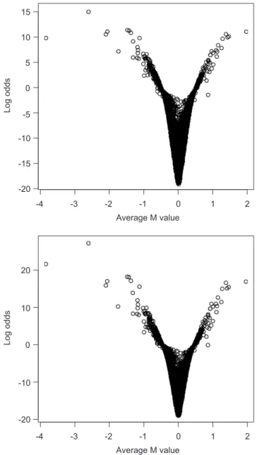
proceeding to simulations. Fig.1 shows a plot of log odds of differential expression versus average

Mvalue withk =log 1.5 for normal and double exponential priors. Again maximized marginal likelihoods strongly indicate that the normal prior (b=2) is more appropriate for the real data. The maximized marginal log likelihood for the normal prior is−246.6 and for the double tailed exponential prior is−375.4. In Fig. 1 for the normal prior there are 430 genes differentially expressed (log odds of differential expression greater than zero). Atk =log 1.25, on the other hand, 2266 genes are declared differentially expressed which is biologically implausible. For the double exponential prior, there are 2261 and 541 genes differentially expressed atkvalues of log 1.25 and log 1.5, respectively. The large number of genes differentially expressed atk=

log 1.25 occurs because of the estimated values ofpof 0.85 and 1.0, respectively for the normal and double exponential priors. Although the data here have been normalized to remove put down time, intensity and print tip effects, it is well known that array speciﬁc effects can interact with

(13)

-4 -3 -2 -1 0 1 2 -20 -15 -10 -5 0 5 10 15 Average M value Log odds -4 -3 -2 -1 0 1 2 -20 -10 0 10 20 Average M value Log odds

Fig. 1. Plot of log odds of differential expression versus averageMvalue for cutoffk=log 1.5 for normal prior (top) and double exponential prior (bottom).

gene effects and it is very difﬁcult to completely adjust for this in normalization. In this example, there is evidence of a large number of small effects so that concentrating on genes with large effects is sensible if the interesting variation of genetic origin is thought to be large compared to the variation of non-genetic origin remaining after normalization. The choice ofk =log 1.5 was based on prior expert opinion about the level of array speciﬁc variation of a non genetic origin.

(14)

Table 3

FDR, FDR–FDR, FNR, FNR– FNR, NFP, NFN and NDE for simulations based on ﬁtted model with normal prior to inbred mice data EBN EBD HBN HBD k=log 1.25 FDR 0.2209 0.2194 0.2210 0.2194 NDE=3407.4 (0.0012) (0.0012) (0.0013) (0.0012) FDR–FDR −0.0004 0.0077 −0.0003 0.0078 (0.0014) (0.0013) (0.0014) (0.0013) FNR 0.0573 0.0576 0.0573 0.0576 (0.0002) (0.0002) (0.0002) (0.0002) FNR–FNR 0.0001 0.0038 0.0000 0.0037 (0.0002) (0.0002) (0.0002) (0.0002) NFP,NFN 752.7,1051.9 747.6,1057.3 753.0,1051.9 747.6,1057.3 k=log 1.5 FDR 0.2560 0.3511 0.2561 0.3513 NDE=429.8 (0.0038) (0.0034) (0.0038) (0.0035) FDR–FDR 0.0033 0.1192 0.0034 0.1192 (0.0038) (0.0032) (0.0038) (0.0032) FNR 0.0089 0.0069 0.0089 0.0069 (0.0001) (0.0001) (0.0001) (0.0001) FNR–FNR 0.0000 −0.0038 0.0000 −0.0038 (0.0001) (0.0001) (0.0001) (0.0001) NFP,NFN 110.0,189.9 150.9,147.2 110.1,189.9 151.0,147.2 k=log 2.0 FDR 0.2683 0.4903 0.2683 0.4911 NDE=18.3 (0.0190) (0.0154) (0.0190) (0.0152) FDR–FDR −0.0162 0.2501 −0.0159 0.2489 (0.0191) (0.0132) (0.0191) (0.0131) FNR 0.0004 0.0003 0.0005 0.0003 (0.0000) (0.0000) (0.0000) (0.0000) FNR–FNR 0.0000 −0.0005 0.0000 −0.0005 (0.0000) (0.0000) (0.0000) (0.0000) NFP,NFN 4.9,8.7 9.0,6.5 4.9,10.9 9.0,6.5

Results of our simulations are shown in Tables3 and 4. Table 3 relates to the normal prior (withc=0.51,p=0.85, the estimates obtained from the real data), and Table 4 to the double exponential prior (withc=1.09,p=1.0, estimates also obtained from the real data). Looking at Table 3 ﬁrst, we see that the results for different priors are substantially similar at low levelsk. At higher levels, the double exponential prior gives a higher FDR and lower FNR and the model based estimate of the FDR performs poorly for the double exponential prior. Looking at the results when the data are simulated using the double exponential prior (Table 4) the conclusions are similar, with the prior used in simulating the data generally performing better. Once again there does not seem to be any great difference between the empirical and hierarchical Bayes analyses. It might be argued that in the two examples considered so far based on ﬁtting to real data sets there seems to be a large number of small effects so that withplarge we can estimate the parameterspand

cfairly well. Hence ignoring the uncertainty about these parameters does not result in any great difference between the empirical and hierarchical Bayes methods. With this in mind we consider

(15)

Table 4

FDR, FDR–FDR, FNR, FNR– FNR, NFP, NFN and NDE for simulations based on ﬁtted model with double tailed exponential prior to RI mice data

EBN EBD HBN HBD k=log 1.25 FDR 0.2026 0.1623 0.2025 0.1620 NDE=2923.8 (0.0012) (0.0011) (0.0012) (0.0011) FDR–FDR 0.0416 0.0020 0.0416 0.0017 (0.0011) (0.0009) (0.0011) (0.0010) FNR 0.0380 0.0442 0.0381 0.0442 (0.0002) (0.0002) (0.0002) (0.0002) FNR–FNR −0.0092 −0.0004 −0.0091 −0.0002 (0.0002) (0.0002) (0.0002) (0.0002) NFP,NFN 592.4,715.9 474.5,592.1 592.1,717.8 473.7,832.7 k=log 1.5 FDR 0.1432 0.1498 0.1430 0.1498 NDE=883.2 (0.0019) (0.0019) (0.0019) (0.0019) FDR–FDR −0.0075 0.0021 −0.0078 0.0019 (0.0018) (0.0017) (0.0018) (0.0017) FNR 0.0111 0.0108 0.0111 0.0108 (0.0001) (0.0001) (0.0001) (0.0001) FNR–FNR 0.0002 −0.0002 0.0003 −0.0002 (0.0001) (0.0001) (0.0001) (0.0001) NFP,NFN 126.5,231.8 1323.3,225.5 126.3,231.8 132.3,225.5 k=log 2.0 FDR 0.0800 0.1306 0.0800 0.1305 NDE=212.8 (0.0027) (0.0033) (0.0028) (0.0033) FDR–FDR −0.0605 −0.0015 −0.0605 −0.0018 (0.0027) (0.0030) (0.0027) (0.0030) FNR 0.0028 0.0021 0.0028 0.0021 (0.0001) (0.0000) (0.0001) (0.0000) FNR–FNR 0.0009 −0.0001 0.0009 −0.0001 (0.0000) (0.0000) (0.0000) (0.0000) NFP,NFN 17.0,60.3 27.8,45.3 17.0,60.3 27.8,45.3

a further example where we ﬁxp =0.02 and estimatecfor the swirl zebraﬁsh data set for the two different priors and then simulate using these parameter values.

4.3. Swirl zebraﬁsh data,p=0.02

Results of simulations for the swirl zebrafish data set where we have fixedp=0.02 are shown in Tables5 and 6. Table 5 relates to simulations done from the normal prior (withc=6.54, the estimate obtained from the real data), and Table 6 to simulations done from the double exponential prior (withc= 0.82, also obtained by fitting to the real data). Conclusions of the hierarchical and empirical Bayes analyses seem to be similar for the prior used in simulating the data for both the cases considered, but not for the alternative prior. When there are few genes differentially expressed and the prior not used in simulating the data is used then in general inference using the hierarchical approach seems to be more conservative.

(16)

Table 5

FDR, FDR–FDR, FNR, FNR– FNR, NFP, NFN and NDE for simulations based on ﬁtted model with normal prior to swirl zebraﬁsh data withp=0.02

EBN EBD HBN HBD k=log 1.25 FDR 0.1641 0.1385 0.1660 0.0958 NDE=108.6 (0.0068) (0.0102) (0.0067) (0.0054) FDR–FDR −0.0011 −0.0396 −0.0006 −0.0654 (0.0059) (0.0095) (0.0059) (0.0054) FNR 0.0066 0.0066 0.0066 0.0075 (0.0001) (0.0001) (0.0001) (0.0001) FNR–FNR 0.0000 −0.0019 0.0000 0.0029 (0.0002) (0.0002) (0.0002) (0.0002) NFP,NFN 17.8,55.0 15.0,55.0 18.0,55.0 10.4,62.5 k=log 1.5 FDR 0.1468 0.1128 0.1475 0.0935 NDE=77.4 (0.0062) (0.0092) (0.0063) (0.0055) FDR–FDR −0.0037 −0.0461 −0.0036 −0.0580 (0.0053) (0.0085) (0.0053) (0.0055) FNR 0.0031 0.0033 0.0031 0.0037 (0.0001) (0.0001) (0.0001) (0.0001) FNR–FNR 0.0000 −0.0002 0.0000 0.0014 (0.0001) (0.0001) (0.0001) (0.0001) NFP,NFN 11.4,25.9 8.7,27.6 11.4,25.9 7.2,31.0 k=log 2.0 FDR 0.1356 0.0921 0.1362 0.1165 NDE=42.7 (0.0079) (0.0092) (0.0081) (0.0078) FDR–FDR 0.0055 −0.0418 0.0051 −0.0500 (0.0067) (0.0088) (0.0063) (0.0067) FNR 0.0011 0.0012 0.0011 0.0013 (0.0000) (0.0001) (0.0000) (0.0000) FNR–FNR 0.0000 0.0001 0.0000 0.0004 (0.0000) (0.0000) (0.0000) (0.0000) NFP,NFN 5.8,9.2 3.9,10.1 5.8,9.2 5.0,10.9

5. Discussion and conclusions

In this paper we have examined frequentist performance of different prior speciﬁcations in empirical and hierarchical Bayes methods for detecting differential expression in simple compar-ative microarray experiments involving two experimental conditions. Empirical and hierarchical Bayes approaches to the analysis of microarray data generally give similar conclusions. Results were sensitive to the prior used when assessing differential expression with effect larger than a certain thresholdkfor largek, which is to be expected since it is for large effects that the shrinkage methods associated with the different priors give the most different results. Generally, however, there was good agreement between analyses for the different priors, and model based estimates of false discovery rates performed well. These conclusions have implications for the analysis of microarray data from experiments with a more complex design than the simple comparative ex-periments considered here. Generally if empirical Bayes methods perform as well as hierarchical

(17)

Table 6

FDR, FDR–FDR, FNR, FNR– FNR, NFP, NFN and NDE for simulations based on ﬁtted model with double tailed exponential prior to swirl zebraﬁsh data withp=0.02

EBN EBD HBN HBD k=log 1.25 FDR 0.1878 0.2963 0.0000 0.2770 NDE=24.3 (0.0368) (0.0408) (0.0000) (0.0405) FDR–FDR 0.0343 0.0671 −0.0178 0.0819 (0.0288) (0.0382) (0.0011) (0.0367) FNR 0.0029 0.0028 0.0032 0.0029 (0.0001) (0.0001) (0.0001) (0.0001) FNR–FNR 0.0007 −0.0010 0.0023 0.0000 (0.0003) (0.0012) (0.0001) (0.0002) NFP,NFN 4.6,24.4 7.2,23.6 0.0,27.0 6.7,24.4 k=log 1.5 FDR 0.1919 0.2807 0.0000 0.2858 NDE=10.4 (0.0369) (0.0396) (0.0000) (0.0418) FDR–FDR 0.0388 0.0827 0.0000 0.0865 (0.0286) (0.0351) (0.0000) (0.0384) FNR 0.0004 0.0011 0.0013 0.0011 (0.0001) (0.0001) (0.0001) (0.0001) FNR–FNR 0.0002 −0.0002 0.0013 0.0001 (0.0001) (0.0002) (0.0001) (0.0001) NFP,NFN 2.0,3.4 2.9,9.3 0.0,11.0 3.0,9.3 k=log 2.0 FDR 0.1970 0.2451 0.0000 0.2387 NDE=4.1 (0.0382) (0.0398) (0.0000) (0.0413) FDR–FDR 0.0566 0.0617 0.0000 0.0688 (0.0283) (0.0347) (0.0000) (0.0356) FNR 0.0004 0.0003 0.0005 0.0003 (0.0000) (0.0000) (0.0000) (0.0000) FNR–FNR 0.0002 0.0000 0.0005 0.0001 (0.0000) (0.0001) (0.0000) (0.0000) NFP,NFN 0.8,3.4 1.0,2.5 0.0,4.2 1.0,2.5

Bayes methods as they do here then it may not be worth the computational overhead to implement the more complex fully hierarchical method.

It would be possible to integrate the process of microarray normalization with as assessment of signiﬁcance as an extension of this work. Recent progress in this direction is described in Lewin et al.[14], Fan et al. [7] and Huang et al. [10]. However, such an approach demands a more complex modelling in which revealing analytical expressions for the log odds of differential expression such as those described in this paper are not available. The desirability of taking into account uncertainty in normalization in subsequent inference for gene effects is undeniable, however.

We have focussed in this paper on priors for the gene specific mean parameters. However, also of interest would be further examination of alternative more flexible prior specifications for the gene variances2_gas an alternative to the inverse gamma prior. One alternative prior would be an inverse gamma mixture, for which the kind of analytic calculations done in this paper could still be carried out. The estimation of prior hyperparameters is more complex, however. The priors

(18)

we have considered on the mean parameters could also be made more ﬂexible. Some interesting recent work in this direction is the semiparametric hierarchical mixture approach of Newton et al.

[19]. However, simple parametric priors of the kind considered here may perform well and allow for calculations to be done analytically.

Acknowledgments

This research was supported by an Australian Research Council grant. Chris Cotsapas was supported by a School of Biotechnology and Biomolecular Sciences Genome Information Schol-arship, Rohan Williams by a National Health and Medical Research Council of Australia Peter Doherty Fellowship, and Mark Cowley and Eva Chan by Australian Postgraduate Awards.

Appendix

We derive the expressions for the marginal likelihoods given in Section 2 and the posterior distribution for_g|_g=0, M. We have that

The integral in (6) is easily done analytically here since the integrand is an unnormalized inverse gamma density. A similar argument gives

p(Mg|g=0)= p(Mg|g =0, 2 g)p( 2 g) d 2 g = −ng 2 _(n₀_s2 0) n₀ 2 _n 0+ng 2 n0 2 ⎛ ⎝n0s20+ j M_gj2 ⎞ ⎠ −n0+ng 2 .

In general, the integral (5) can be done numerically in order to calculate Pr(_g = 0|M). However, in the case whereb =2 (a normal prior) orb=1 (a double tailed exponential prior)

(19)

some further analytic simpliﬁcation is possible. For the normal case, we have p(Mg|g=0)= G(_g,2, c, n0, s02) dg = K(2, c, n0, s02) ⎛ ⎝n0s02+ 2 g c + j (Mgj−g)2 ⎞ ⎠ −n0+ng+1 2 d_g, where K(2, c, n0, s02)= −ng2 _(n₀_s2 0) n0 2 n0+ng+1 2 √ cn0 2 .

To evaluate the integral here and a similar integral for the case of the double tailed exponential prior (b=1) we use the following lemma.

Lemma 1. For constantsf, gandh >0withf h > g2

A (f −2gt+ht2)−(+21) _dt= f −g 2 h − 2 h−12_B 1 2, 2 Pr(T ∈A),

whereB(·,·)is the beta function and T ∼t g h, 1 h f −g 2 h ,

wheret(,2)denotes the t-distribution withdegrees of freedom,meanand scale parame-ter2.

Proof. The proof is straightforward upon recognizing the integrand as an unnormalizedt-density,

t g h, 1 h f −g_h2 .

Applying this lemma here for theb=2 normal prior case gives

p(Mg|g=0)= −ng 2 (n₀s2 0) n₀ 2 n0+ng 2 (cng+1) 1 2n0 2 ⎛ ⎝n0s02+ j M_gj2− cng 1+cng ngM¯g2 ⎞ ⎠ −n₀+ng 2 ,

which is the expression in Lönnstedt and Speed[13] and Smyth [21]. We can use Lemma 1 to obtain an expression forp(Mg|g=0)also in the case whereb=1 (the double tailed exponential prior). Here p(Mg|g=0)= G(_g,1, c, n0, s02) dg =K(1, c, n0, s02) ⎛ ⎝n0s20+ |g| c + j (Mgj −g)2 ⎞ ⎠ −n0+ng+2 2 d_g,

(20)

where K(1, c, n0, s02)= −ng 2 _(n₀_s2 0) n₀ 2 _n 0+ng+2 2 2cn0 2 .

In the notation of Section 2 we write the integral as I1+I2 and obtain the expressions for

I1 andI2 given in Section 2 upon applying Lemma 1 if (3) holds. If (3) does not hold, then

p(Mg|g=0)cannot be written in terms of distribution functions ofTrandom variables, but the required integrations can be done using some standard numerical integration method.

We also need the posterior distribution ofggiveng=0 in order to calculate (2). Note that p(_g|Mg,g=0)= p(_g,2_g|Mg,g=0) d2g ∝ p(2_g)p(_g|2_g)p(Mg|g,2g) d 2 g = G(_g, b, c, n0, s02).

Whenb=2 (a normal prior) we have thatG(_g,2, c, n0, s02)is proportional to at-density,

tn0+ng cng 1+cng ¯ Mg, cng 1+cng n0s02+ jMgj2 − cng 1+cngngM¯ 2 g ng(n0+ng) . (7)

In the case ofb=1 (the double tailed exponential prior)

p(_g|Mg,g=0) ∝G(_g,1, c, n0, s02) = −ng2 _(n₀_s2 0) n0 2 n0+ng+2 2 2cn0 2 ⎛ ⎝n0s0+2 |g| c + j (Mgj−g)2 ⎞ ⎠ −n0+ng+2 2 .

If (3) holds, this density is a mixture of two constrainedt-densities as described in Section 2.

References

[1]H. Akaike, Information theory and an extension of the maximum likelihood principle, Second International Symposium on Information Theory, 1973, pp. 267–281.

[2]P. Baldi, A.D. Long, A Bayesian framework for the analysis of microarray data: regularized t-test and statistical inferences of gene changes, Bioinformatics 17 (2001) 509–519.

[3]Y. Benjamini,Y. Hochberg, Controlling the false discovery rate: a practical and powerful approach to multiple testing, J. Roy. Statist. Soc. B 57 (1995) 289–300.

[4]P. Broët, S. Richardson, F. Radvanyi, Bayesian hierarchical model for identifying changes in gene expression from microarray experiments, J. Comput. Biol. 9 (2002) 671–683.

[5]C. Cotsapas, E. Chan, M. Kirk, M. Tanaka, P. Little, Genetic variation in the control of transcription, Cold Spring Harbor Symposia on Quantitative Biology, vol. 68, 2003, pp. 109–114.

[6]S. Dudoit, Y.H. Yang, Bioconductor R packages for exploratory analysis and normalization of cDNA microarray experiments, in: G. Parmigiani, E.S. Garrett, R. Izirarry, S.L. Zeger (Eds.), The Analysis of Gene Expression Data: Methods and Software, Springer, New York, 2003, pp. 73–101.

[7]J. Fan, H. Peng, T. Huang, Semilinear high-dimensional model for normalization of microarray data: a theoretical analysis and partial consistency (with discussion), J. Amer. Statist. Assoc. 100 (2005) 781–813.

[8]D.P. Foster, E.I. George, The risk inﬂation criterion for multiple regression, Ann. Statist. 22 (1994) 1947–1975. [9]E.I. George, D.P. Foster, Calibration and empirical Bayes variable selection, Biometrika 87 (4) (2000) 731–747.

(21)

[10]J. Huang, D. Wang, C. Zhang, A two-way semilinear model for normalization and analysis of cDNA microarray data, J. Amer. Statist. Assoc. 100 (2005) 814–829.

[11]J.G. Ibrahim, M. Chen, R.J. Gray, Bayesian models for gene expression with DNA microarray data, J. Amer. Statist. Assoc. 97 (2002) 88–99.

[12]G. Kauermann, P. Eilers, Modelling microarray data using a threshold mixture model, Biometrics 60 (2004) 376–387.

[13]C.M. Kendziorski, M.A. Newton, H. Lan, M.N. Gould, On parametric empirical Bayes methods for comparing multiple groups using replicated gene expression proﬁles, Statist. Med. 22 (2003) 3899–3914.

[14]A. Lewin, S. Richardson, C. Marshall, A. Glazier, T. Aitman, Bayesian modelling of differential gene expression, Biometrics 62 (2006) 10–18.

[15]J.S. Liu, Monte Carlo Strategies in Scientiﬁc Computing, Springer, New York, 2001.

[16]I. Lönnstedt, S. Grant, G. Begley, T.P. Speed, Microarray analysis of two interacting treatments: a linear model and trends in expression over time, Technical Report, Department of Mathematics, University, 2003. Available at www.math.uu.se/staff/pages/?uname-ingrid.

[17]I. Lönnstedt, T.P. Speed, Replicated microarray data, Statist. Sinica 12 (2002) 31–46.

[18]M.A. Newton, C.M. Kendziorski, Parametric empirical Bayes methods for microarrays, in: G. Parmigiani, E.S. Garrett, R. Izirarry, S.L. Zeger (Eds.), The Analysis of Gene Expression Data: Methods and Software, Springer, New York, 2003.

[19]M.A. Newton, A. Noueiry, D. Sarkar, P. Ahlquist, Detecting differential gene expression with a semiparametric hierarchical mixture method, Biostatistics 5 (2004) 155–176.

[20]G. Schwartz, Estimating the dimension of a model, Ann. Statist. 6 (1979) 461–464.

[21]G.K. Smyth, Linear models and empirical Bayes methods for assessing differential expression in microarray experiments, Statist. Appl. Genetics Molecular Biol. 3 (2004) 1–25.