Geocoding Large Population-level Administrative Datasets
at Highly Resolved Spatial Scales
Sharon E. Edwards,* Benjamin Strauss
†and Marie Lynn Miranda*
,‡*Children’s Environmental Health Initiative, University of Michigan †Nicholas School of the Environment, Duke University
‡Department of Pediatrics, University of Michigan
Abstract
Using geographic information systems to link administrative databases with demographic, social, and environmental data allows researchers to use spatial approaches to explore relationships between expo-sures and health. Traditionally, spatial analysis in public health has focused on the county, ZIP code, or tract level because of limitations to geocoding at highly resolved scales. Using 2005 birth and death data from North Carolina, we examine our ability to geocode population-level datasets at three spatial resolu-tions – zip code, street, and parcel. We achieve high geocoding rates at all three resoluresolu-tions, with statewide street geocoding rates of 88.0% for births and 93.2% for deaths. We observe differences in geocoding rates across demographics and health outcomes, with lower geocoding rates in disadvantaged populations and the most dramatic differences occurring across the urban-rural spectrum. Our results suggest that highly resolved spatial data architectures for population-level datasets are viable through geocoding individual street addresses. We recommend routinely geocoding administrative datasets to the highest spatial resolution feasible, allowing public health researchers to choose the spatial resolution used in analysis based on an understanding of the spatial dimensions of the health outcomes and exposures being investigated. Such research, however, must acknowledge how disparate geocoding success across subpopulations may affect findings.
1 Introduction
Geographic Information Systems (GIS) and spatial analysis are of growing importance in public health research, outreach, and policy. The increasing availability and evolving method-ologies of GIS technology and spatial statistics enable researchers to explore the connections between public health endpoints and relevant demographic, social, and environmental condi-tions by integrating across previously disparate datasets (Krieger et al. 2005; Mindell and Barrowcliffe 2005; Bergquist and Rinaldi 2010; Robinson et al. 2010; Comer et al. 2011; Eisen and Eisen 2011; Miranda and Edwards 2011; Goldberg and Jacquez 2012).
Administrative datasets, such as birth certificates, immunizations, student enrollments, notifiable diseases, and death records, are an important resource for public health researchers, as these data often cover large populations and extended periods of time. Using GIS to display these data can reveal spatial patterns which may help generate hypotheses for future research,
Address for correspondence:Marie Lynn Miranda, Children’s Environmental Health Initiative, School of Natural Resources and Environ-ment, University of Michigan, 2046 Dana Building, 440 Church Street, Ann Arbor, MI 48109, USA. E-mail: [email protected] Acknowledgements: This work was supported by grants from the US Environmental Protection Agency (RD-83329301) and from the National Center for Research Resources (UL1RR024128), a component of the National Institutes of Health and the NIH Roadmap for Medical Research. Funding agencies were not involved in the decisions regarding this article or the analysis it presents. We are grateful for the data management provided by Claire Osgood and the geocoding efforts of Nancy Schneider.
provide information for targeting community outreach, or motivate policy efforts and prior-ities. Using GIS to link these administrative databases with relevant demographic, social, and environmental data via shared geography can allow for spatial statistical approaches to explore relationships between exposures and health endpoints. With key administrative datasets containing information covering many years, these data may be even more valuable in that they can enable spatio-temporal analysis of health outcomes as populations shift and exposures change over time.
Geocoding, the process of converting address information into latitude and longitude coordinates, is the key to leveraging the valuable information already collected in administra-tive datasets for use in spatial analyses. Four key measures of geocoding quality have been identified: completeness, resolution, matching algorithm criteria, and positional accuracy (Goldberg and Jacquez 2012). Much of the research on geocoding has focused on the posi-tional accuracy of different geocoding techniques (Krieger et al. 2001; Ratcliffe 2001; Bonner et al. 2003; Cayo and Talbot 2003; Bow et al. 2004; Ward et al. 2005; Duncan et al. 2011; Bell et al. 2012; Goldberg and Cockburn 2012; Healy and Gilliland 2012; Jacquez 2012). Errors in positional accuracy can lead to incorrect assignment of areal units such as Census tract or even county, leading to misclassification errors (Goldberg and Cockburn 2012; McLafferty et al. 2012). Completeness of geocoding and matching algorithm criteria are diffi-cult to compare across many studies due to a lack of detail describing the geocoding process in many papers (Robinson et al. 2010).
At least three important advances have occurred that can lead to improvements in geocoding of administrative datasets: (1) address information in administrative datasets has become more complete and standardized; (2) reference layers have been updated, standard-ized, and more completely populated (Rushton et al. 2006); and (3) geocoding processes and methodologies have improved (Zandbergen and Chakraborty 2006; Goldberg et al. 2007). Inevitably, however, there are records in any dataset that cannot be geocoded, and understand-ing systematic issues in geocodunderstand-ing completeness is important for understandunderstand-ing the types of research that can be undertaken with a particular dataset and the bias to which such research may be subject.
In this article, we focus on two of the key measures of geocoding affected by these advances: completeness and spatial resolution. Focusing on 2005 birth and death certificate data from the State of North Carolina, we explore our ability to construct complete spatial datasets for large population-level administrative datasets at highly resolved spatial scales. If we are able to geocode administrative datasets thoroughly and at refined spatial scales, this will have important implications for the spatial scale at which public health research can be undertaken. Using data for the entire state, we assess geocoding completeness, or match rates, at different spatial resolutions across various subpopulations and regions.
2 Methods
2.1 Data
We used two large administrative datasets from North Carolina (NC) – the detail birth record (DBR) and the detail death record (DDR). Through a data sharing agreement, the NC State Center for Health Statistics provided individually-identified birth and death record data with key demographic, health, and geographic variables for all births and deaths occurring in North Carolina in 2005. Each record provided geographic information that was collected at the time of the birth or death, including county of residence, ZIP code, and street address. Note that
the street address provided in the DBR is actually the mailing address, with a variable to indi-cate if this was also the residential address. Quality of the DBR data has been studied and reported elsewhere (Buescher et al. 1993; Vinikoor et al. 2010), with studies indicating demo-graphic and outcome data is fairly well recorded. No studies were available on the quality of the DDR data.
Race, age, education, marital status, and select health outcome variables provided in the DBR and DDR allowed us to examine trends in geocoding rates in the state overall, as well as within demographic subgroups. Births and deaths were subsetted by race into non-Hispanic white (NHW), non-Hispanic black (NHB), Hispanic (H), and Asian/Pacific Islander (A/PI); all records falling into other race categories were dropped from race-stratified analysis due to small sample size. Educational attainment of the decedent (DDR) and of the mother (DBR) was
classi-fied as less than 9th grade, some high school, high school degree, some college, and college
degree+. For the DBR, maternal age was classified into 5-year age groups for those women aged
15–44. For the DDR, the age of the decedents was classified as<20 years, 20–29 years, 30–39
years, 40–49 years, 50–59 years, 60–69 years, 70–79 years, 80–89 years, and≥90 years. Preterm
birth (<37 weeks gestational age at delivery) and diabetes-related death were selected as example
public health outcomes to which geospatial analysis might be applied.
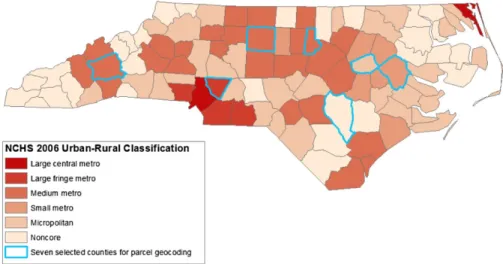
In addition, we used data from the National Center for Health Statistics (NCHS) to assign each birth and death an urbanization level based on the reported county of residence. The NCHS classifies all US counties into one of six levels of urbanization: large central metro, large fringe metro, medium metro, small metro, micropolitan (nonmetro), and noncore (nonmetro) (US Centers for Disease Control and Prevention et al. 2012). Figure 1 shows the distribution of these urbanization levels across NC.
2.2 Geocoding
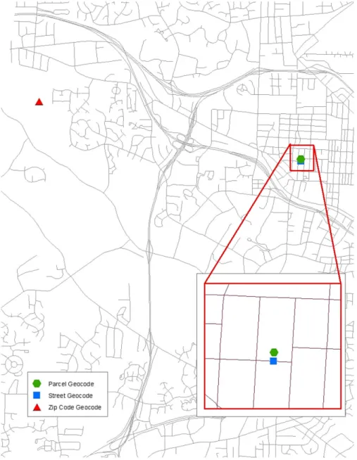
Residential addresses were geocoded using Esri ArcGIS 9.3 (Redlands, California) at three levels of spatial resolution – ZIP code, street, and parcel. Figure 2 displays how the same address would be spatially located using the three methods. Geocoding to an areal unit (e.g.
Figure 1 County urban-rural designations as classified by the National Center for Health Statistics (NCHS) and the seven counties selected for parcel geocoding
ZIP code or parcel) typically assigns an address the latitude and longitude of the centroid of the areal unit with the corresponding address information. Street geocoding places the obser-vation proportionally along a street segment, taking into account the address range of the street segment and the street number of the address. Rushton et al. (2006) provide a more in-depth description of how spatial location is assigned during the geocoding process.
The US Census Zip Code Tabulation Area 2000 geography (US Census Bureau 2012) was used as the reference layer for ZIP code level geocoding. Only records with a ZIP code that exactly matched a ZIP code in the reference layer were geocoded.
Street level geocoding located residential street addresses based on the 2006 Topologically Integrated Geographic Encoding and Referencing system (TIGER) street centerlines file (US Census Bureau and Geography Division 2007). Similar to the manual geocoding improvement approach (Goldberg et al. 2008), street level geocoding occurred in three batches. First, we geocoded addresses that exactly matched to the road reference layer’s street address compo-nents. Unmatched addresses from this first batch were standardized to be more compatible with the road reference layer by removing apartment, unit, suite, and lot numbers; formatting highways and routes numbers; and obtaining street addresses for common apartment com-plexes, housing developments, and mobile home parks. For the second batch, we geocoded those standardized addresses matching exactly to street address components in the reference layer. The final batch required a GIS technician to examine candidate matches for all remain-ing unmatched records and select candidate matches for geocodremain-ing when appropriate. An inexact match might be selected as the geocoded location for a DBR or DDR record due to, for example, spelling errors in an address; incorrect street type or direction; and units within housing developments, apartment complexes, or mobile home parks.
The parcel geocoding process referenced data provided by county tax assessor offices in order to assign records to individual tax parcels based on the physical address of each parcel (i.e. not the owner’s mailing address). Geocoding to the tax parcel level was done using the same three tiered batch process described above (exact matches with original address, exact matches with standardized address, and hand matching).
ZIP code and street level geocoding were performed statewide for both the DBR and DDR data; however, parcel geocoding could not be undertaken statewide as not all NC counties have developed GIS layers of their tax parcel data and reporting of physical address within parcel data varies by county. The seven most rural counties in NC did not have any parcel GIS data, and rural counties also included physical address in parcel data less frequently than more urban counties. Thus, parcel geocoding of births and deaths was undertaken in seven select North Carolina counties: Buncombe, Cabarrus, Durham, Guilford, Pitt, Sampson, and Wilson. These counties are highlighted in Figure 1. While additional counties have developed tax parcel GIS layers, these seven counties were chosen for their distribution across the state and as examples of geographic areas with different levels of urbanization. In order from most urban to most rural, these counties are classified as large fringe metro (Cabarrus), medium metro (Buncombe, Durham, Guilford), small metro (Pitt), micropolitan (Wilson), and noncore (Sampson).
While ZIP code geocoding was undertaken for all records, street and parcel level geocoding were only undertaken for those records for which a residential street address was reported. Records were considered to be missing residential street address if the address field was blank, only a mailing address was provided, a partial street name was provided, a post office box was reported, or rural route box was reported. Missing addresses were identified manually. The inclusion of a residential street address in a record does not guarantee the address can be geocoded. Records may not be able to be geocoded due to incomplete residen-tial address (e.g. missing street direction or type), incomplete reference layer data, or inability to determine the address of a multi-residence facility. The geocoding match rate is defined as the proportion of all records (both those reporting and those not reporting an address) that were able to be successfully assigned a spatial location at a specific spatial resolution.
2.3 Statistical Analysis
We tested for differences in reporting of residential street address and geocoding match rates across demographic (race, age, education, marital status, and urbanization) and outcome
(preterm birth for births and diabetes-related death for deaths) subgroups using Chi-squared tests. For both births and deaths, differences in address reporting and geocoding rates were assessed for each level of geocoding – ZIP code, street, and parcel (select counties only). Since this analytic approach required conducting a large number of tests, we would expect to find significant results purely by chance. To address this issue and be more confident that our results highlight true differences in reporting and geocoding rates, we calculated adjusted p-values using the false discovery rate (FDR) method of controlling error under multiple com-parisons. This method controls for the expected proportion of tests that are incorrectly identi-fied as significant, and attempts to balance the desire for power to identify true difference and the desire to be conservative in falsely identifying tests as significant. For the DBR and DDR analyses separately, the false discovery rate was controlled at 0.05, thus tests with adjusted p-values less than 0.05 were considered significant and we could expect that, on average, 5% of the differences found may not actually be significant.
3 Results
In 2005, there were 121,248 births and 73,016 deaths reported in North Carolina’s detailed birth and death records, respectively. Tables 1 and 2 present the distribution of births and deaths, respectively, across demographic subgroups, as well as residential street address report-ing rates within each group. Most births were to mothers who were NHW, less than 30 years old, married, and with at least a high school education. Most deaths were of individuals who were 60 years of age or older, not married, and with at least a high school education. Both births and deaths were most commonly among residents of medium metro and micropolitan counties.
3.1 Address Reporting
The proportion of records that included a residential street address represent an upper limit on geocoding match rates for street and parcel level geocoding efforts (ZIP code geocoding only requires a ZIP code, not a full street address). Statewide, 92.7% of birth records and 99.2% of death records included a residential street address. In the DBR, missing addresses were pre-dominantly due to reporting of mailing address rather than residential address (95%). In the death data, post office and rural route boxes accounted for almost half of the records missing addresses, with partial addresses accounting for 42% and no street address information for 8% of these records.
Birth and death records from more rural areas were less likely to include a street address
(FDR-adjusted p<0.05); however, while address reporting rates in the death record remained
above 98% in all urban-rural classifications, the reporting rate in the birth record dropped to as low as 73.5% in non-core counties. Address reporting among births varied by maternal
race, age, education, and marital status (FDR-adjusted p<0.5). Generally, births to women at
higher risk for adverse pregnancy outcomes – minority women, extremely young or old mothers, women with low educational attainment, and single women – were less likely to report a street address in the DBR. Preterm births were also slightly less likely to report a street address than were term births (92.9% for term versus 92.0% for preterm births;
FDR-adjusted p < 0.05). In the death record data, although there were differences in residential
street address reporting by race, age, marital status, and education (FDR-adjusted p<0.5),
Table 1 Counts of records and percent repor ting a residential street ad dress fo r 2005 bir ths in NC and select counties a Statewide Buncombe County Cabar rus County Durham County Guilf ord County Pitt County Sampson County Wilson County N % with ad dress N % with ad dress N % with ad dress N % with ad dress N % with ad dress N % with ad dress N % with ad dress N % with ad dress All 121,248 92.7 2,587 90.5 2,365 98.4 4,038 98.3 5,956 99.1 2,016 94.5 929 81.0 1,043 90.9 Maternal race/ethnicity NHW 68,856 93.8 2,013 89.5 1,516 98.4 1,454 98.1 2,629 99.1 978 95.4 400 92.5 399 93.2 NHB 27,777 91.4 192 93.8 327 97.3 1,368 97.9 2,189 99.2 818 92.8 226 84.1 424 89.6 Hispanic 19,437 91.4 331 94.3 463 98.9 967 99.1 822 99.3 180 96.1 279 60.6 208 88.5 Other 5,039 91.0 46 95.7 57 98.3 237 98.7 314 99.4 40 100.0 23 95.7 12 100.0 Maternal age(yrs) 15–19 13,684 89.9 284 88.0 202 97.5 376 98.9 559 99.1 235 90.6 115 84.4 166 92.8 20–24 32,165 91.6 696 90.1 575 99.0 828 98.8 1,427 99.3 516 93.8 300 82.3 293 87.4 25–29 32,867 93.1 669 90.7 671 99.0 1,126 98.9 1,603 99.1 609 94.9 268 81.7 284 94.4 30–34 27,263 94.2 581 90.9 588 97.6 1,110 97.1 1,497 99.1 444 95.3 173 76.9 187 87.7 35–39 12,515 94.7 274 92.0 286 97.6 488 98.4 727 99.3 169 97.6 61 77.1 97 93.8 40–44 2,381 92.8 68 92.7 36 100.0 92 97.8 131 97.0 35 97.1 11 72.7 14 92.9 Maternal education < 9th grade 8,956 89.3 148 90.5 172 100.0 456 98.5 404 99.5 128 92.2 149 63.8 115 87.8 Some high school 19,206 89.8 441 87.8 342 98.0 606 99.3 816 99.8 326 92.9 163 75.5 218 92.2 High school 34,506 91.3 737 87.9 647 97.8 755 98.3 1,462 99.1 410 93.4 314 83.4 329 87.5 Some colleg e 26,272 93.2 502 91.6 563 98.6 543 97.1 1,364 98.6 548 93.6 207 89.4 192 92.7 Colleg e degree 32,093 96.6 754 93.9 640 98.4 1,661 98.4 1,905 99.2 602 97.3 92 91.3 189 95.2 Maternal marital status Mar ried 74,755 94.3 1,616 91.0 1,615 98.7 2,351 98.1 3,511 99.2 1,090 95.2 494 84.4 505 92.5 Not mar ried 46,489 90.2 970 89.7 750 97.6 1,687 98.6 2,445 99.0 926 93.6 435 77.0 538 89.4 Gestational age at deli very Term bir th 105,507 92.9 2,260 90.9 2,066 98.4 3,545 98.4 5,166 99.2 1,705 94.8 799 79.9 895 91.0 Preterm bir th 15,678 92.0 326 87.7 298 98.3 492 98.0 785 99.1 311 92.9 130 87.7 147 91.2 Urban-rur al classification Larg e central metro 13,428 98.9 Larg e fring e metro 7,902 95.2 Medium metro 55,449 95.9 Small metro 10,937 93.6 Micropolitan 25,174 87.8 Noncore 8,358 73.5 aGray shading highlights repor ting rates that w ere significantly different (false discov er y rate adjusted p-value < 0.05) across demographic or outcome subgroups
Table 2 Counts of records and percent repor ting a residential street ad dress fo r 2005 deaths in NC and select counties a Statewide Buncombe County Cabar rus County Durham County Guilf ord County Pitt County Sampson County Wilson County N % with ad dress N % with ad dress N % with ad dress N % with ad dress N % with ad dress N % with ad dress N % with ad dress N % with ad dress All 73,016 99.2 2,195 99.3 1,277 99.8 1,653 99.4 3,618 99.8 1,099 99.0 587 99.3 772 99.6 Race/ethnicity NHW 55,922 99.3 2,004 99.3 1,100 99.8 956 99.9 2,611 99.9 634 99.2 376 99.5 472 99.8 NHB 15,461 98.9 171 99.4 168 100.0 661 99.1 944 99.7 457 98.7 188 98.9 285 99.3 Hispanic 573 96.0 10 100.0 5 100.0 17 94.1 20 100.0 3 100.0 10 100.0 13 100.0 Other 1,040 98.5 9 100.0 4 100.0 18 94.4 43 100.0 5 100.0 13 100.0 2 100.0 Age(yrs) < 20 1,758 99.0 49 98.0 23 100.0 46 97.8 89 100.0 40 97.5 14 100.0 19 94.7 20–29 1,216 98.3 36 100.0 14 100.0 35 94.3 59 100.0 15 93.3 12 100.0 14 100.0 30–39 1,764 98.9 43 97.7 27 100.0 39 97.4 78 100.0 33 100.0 13 100.0 19 100.0 40–49 4,093 98.9 127 98.4 69 100.0 98 98.0 185 100.0 66 100.0 33 97.0 44 100.0 50–59 7,421 99.1 193 97.9 126 100.0 181 100.0 352 99.7 129 98.5 63 98.4 94 100.0 60–69 10,429 99.2 275 99.6 173 100.0 212 99.1 472 99.6 179 100.0 77 100.0 110 100.0 70–79 16,568 99.4 456 99.8 292 100.0 333 100.0 768 100.0 250 98.8 145 100.0 172 100.0 80–89 20,707 99.2 683 99.4 385 99.5 501 99.8 1,079 99.8 278 98.9 161 100.0 208 99.0 > 89 9,051 99.1 333 99.4 168 100.0 207 100.0 536 99.6 109 99.1 69 97.1 92 100.0 Education < 9th grade 16,319 98.9 404 99.5 276 99.6 265 99.3 641 99.5 270 98.5 166 99.4 221 99.1 Some high school 15,189 99.1 440 99.6 310 100.0 314 98.7 672 99.9 241 97.9 142 100.0 174 100.0 High school 22,037 99.3 620 98.6 416 100.0 486 99.8 1,120 100.0 305 99.3 165 98.8 221 100.0 Some colleg e 9,861 99.5 336 99.4 171 100.0 257 100.0 559 100.0 140 100.0 67 100.0 84 100.0 Colleg e degree 8,276 99.5 375 100.0 89 100.0 297 100.0 581 99.8 130 100.0 32 96.9 54 98.2 Marital status Mar ried 28,587 99.4 813 99.3 521 100.0 620 99.8 1,357 100.0 380 99.0 207 100.0 276 100.0 Not mar ried 44,294 99.0 1,379 99.3 754 99.7 1,030 99.3 2,257 99.7 717 99.0 379 98.9 495 99.4 Cause of death Not diabetes-related 64,846 99.2 2,033 99.3 1,161 99.8 1,496 99.4 3,250 99.8 942 99.0 520 99.2 668 99.6 Diabetes-related 8,170 99.2 162 99.4 116 100.0 157 99.4 368 99.7 157 98.7 67 100.0 104 100.0 Urban-rur al classification Larg e central metro 4,723 99.6 Larg e fring e metro 4,486 99.1 Medium metro 30,821 99.5 Small metro 6,018 98.7 Micropolitan 19,283 99.1 Noncore 7,685 98.0 aGray shading highlights repor ting rates that w ere significantly different (false discov er y rate adjusted p-value < 0.05) across demographic or outcome subgroups
Among the seven counties selected for parcel geocoding, residential street address report-ing in the birth data generally followed the statewide pattern of more urban areas havreport-ing higher reporting rates than more rural areas; however, address reporting among births in Bun-combe County, a medium metro area, was more on par with Wilson County, a micropolitan area, than with other medium metro counties. Among births in Sampson and Buncombe Counties, differences in address reporting across race/ethnicity were observed, with Hispanic women in Sampson County and NHW women in Buncombe County having lower levels of
address reporting (FDR-adjusted p< 0.5). In Durham County, births to older mothers were
less likely to report a street address (FDR-adjusted p<0.5). In Buncombe, Pitt, and Sampson
Counties, reporting rates in the DBR generally increased with education (FDR-adjusted p <
0.5). In all seven of these counties, address reporting rates for the death record were at least 99%. Reporting rates among younger decedents and those of Hispanic ethnicity were lower in
Durham County (FDR-adjusted p<0.5), but no other differences in address reporting across
demographic and outcome subgroups within these counties were noted.
3.2 ZIP Code Geocoding
ZIP code geocoding rates were high (see Tables 3 and 4), with 96.8% of births and 97.7% of deaths able to be geocoded at this level of spatial resolution. While geocoding rates did vary by
race, age, education (in DDR only), marital status, and urbanization (FDR-adjusted p<0.5),
differences across subgroups were small, within±3 percentage points. Among the seven
coun-ties selected for closer examination, Buncombe County had the lowest ZIP code geocoding rate for births at 96.5% and Durham County had the lowest rate for deaths at 97.5%. In Durham County, small differences in ZIP code geocoding rates across race, age, and education
were observed (FDR-adjusted p<0.5).
Over 500 ZIP codes reported in either the DBR or DDR were not able to be geocoded. ZIP codes were not geocoded because they were not in NC (42% of the unmatched ZIP codes), not real ZIP codes (16% of the unmatched ZIP codes), or not found in the NC ZCTA data (42% of the unmatched ZIP codes). Non-geocoded ZIP codes that actually exist in NC were distributed across the state, occurring in 67 of the 100 NC counties; however, there were clusters of these ZIP codes in the most urban areas of NC, including Mecklenburg, Wake, Forsyth, and Guilford Counties. These ZIP codes may have been established since the 2000 ZCTA data were created.
Births and deaths in counties with parcel data that included data on the physical address of each parcel (i.e. could potentially be used for geocoding) were slightly less likely to be geocoded at the ZIP code level than births and deaths in counties lacking parcel data. For example, 96.3% of births in counties with parcel data that included an address were geocoded, while 97.1% of births in counties without such data were geocoded. This may reflect the creation of new ZIP codes in urban areas that typically have more complete parcel data.
3.3 Street Geocoding
County street-level geocoding rates for both the DBR and DDR data are displayed in Figures 3a–b. The maps are drawn on the same legend using a monochromatic chloropleth in which higher geocoding rates are represented by darker shading and lower geocoding rates are represented by lighter shading. As highlighted by the darker overall color of the map in Figure 3b (death data) compared to the map in Figure 3a (birth data), street geocoding rates were higher for the death record (93.2%) than the birth record (88.0%). Both maps also
Table 3 Geocoding match rates (percent of records g eocoded) at the ZIP code (Zip), street (str), and parcel (parc) lev el among 2005 bir ths a Statewide Buncombe County Cabar rus County Durham County Guilf ord County Pitt County Sampson County Wilson County Zip Str Zip Str P arc Zip Str P arc Zip Str P arc Zip Str P arc Zip Str P arc Zip Str P arc Zip Str P arc All 96.8 88.0 97.5 83.5 83.6 99.6 89.9 92.1 97.8 93.4 95.5 99.4 97.5 93.5 98.6 86.9 80.2 98.7 76.5 39.8 99.4 82.1 82.9 Maternal race/ethnicity NHW 96.5 89.7 97.5 82.9 83.4 99.6 91.0 92.4 96.1 94.5 94.6 99.5 97.8 94.0 99.0 89.6 82.2 100.0 88.5 44.8 99.8 86.0 84.0 NHB 97.2 86.2 97.9 87.5 88.5 99.1 85.6 92.4 98.5 92.0 95.8 99.2 97.6 93.2 98.5 83.4 78.9 98.2 77.9 46.0 99.1 80.9 83.7 Hispanic 97.6 85.5 98.2 84.6 81.0 99.8 90.1 90.7 99.2 94.5 95.8 99.4 96.6 92.8 96.7 86.1 74.4 97.1 56.6 26.2 99.5 76.9 78.4 Other 95.6 84.4 97.8 87.0 93.5 100.0 86.0 93.0 97.9 90.7 98.3 99.4 96.8 93.6 100.0 95.0 85.0 100.0 95.7 56.5 100.0 83.3 100.0 Maternal age(yrs) 15–19 97.0 84.4 96.5 79.9 78.2 99.5 91.6 88.1 99.7 93.9 95.0 99.1 97.1 94.5 97.9 81.3 75.7 97.4 79.1 38.3 100.0 78.3 83.1 20–24 97.5 86.1 98.3 81.2 81.5 99.8 91.8 91.1 98.9 93.7 94.7 99.3 97.3 93.5 98.1 86.2 74.6 99.3 77.7 38.3 99.7 81.2 78.2 25–29 97.0 88.3 97.3 81.9 83.0 99.9 89.3 93.1 98.1 92.7 97.0 99.6 97.6 92.9 98.9 87.5 81.9 98.9 78.7 42.9 98.9 85.9 85.6 30–34 96.0 90.2 97.3 86.4 87.1 99.2 87.1 92.4 96.1 92.5 94.8 99.3 97.5 93.6 98.9 88.3 84.5 98.8 73.4 35.3 99.5 80.8 84.5 35–39 96.1 91.0 97.5 88.0 87.6 99.3 92.7 94.1 97.1 95.7 95.9 99.6 98.2 93.8 99.4 90.5 85.2 98.4 65.6 49.2 99.0 86.6 87.6 40–44 95.8 89.0 100.0 92.7 86.8 100.0 83.3 94.4 97.8 95.7 93.5 99.2 97.0 95.4 100.0 85.7 82.9 90.9 72.7 45.5 100.0 57.1 78.6 Maternal education < 9th grade 97.7 82.3 99.3 79.7 76.4 100.0 92.4 91.3 99.8 94.1 94.1 99.3 95.3 92.6 96.9 79.7 71.1 98.7 60.4 30.9 100.0 78.3 78.3 Some high school 97.3 84.0 96.8 78.7 77.3 99.7 91.5 90.6 99.3 94.1 95.5 99.5 98.2 95.8 98.2 85.3 76.1 96.3 70.6 33.1 99.5 78.9 80.3 High school 97.2 86.3 97.0 80.7 79.8 99.1 90.7 89.0 98.5 93.6 94.8 99.1 97.0 93.0 98.8 85.4 74.6 98.7 78.3 39.2 99.4 81.8 83.0 Some colleg e 97.0 88.9 97.6 84.3 87.7 99.8 90.8 92.9 98.2 91.7 94.7 99.5 97.7 92.2 98.2 85.6 79.6 100.0 86.5 44.4 99.0 83.9 83.9 Colleg e degree 95.7 93.1 98.1 89.1 89.7 99.7 86.9 95.5 96.3 93.5 96.5 99.5 98.0 94.1 99.5 91.4 88.9 100.0 85.9 57.6 99.5 86.8 87.8 Maternal marital status Mar ried 96.4 90.0 97.7 84.2 84.7 99.7 89.4 92.8 96.8 93.5 95.3 99.5 97.6 93.2 98.8 89.0 83.3 99.4 80.4 42.1 99.6 84.6 84.8 Not mar ried 97.4 84.7 97.4 82.4 81.9 99.3 90.9 90.5 99.2 93.3 95.7 99.2 97.3 94.0 98.4 84.3 76.6 97.9 72.2 37.2 99.3 79.7 81.2 Gestational age at deli very Term bir th 96.8 88.1 97.7 83.9 84.3 99.6 89.7 92.0 97.8 93.7 95.6 99.4 97.4 93.7 98.6 87.2 80.1 98.6 75.6 39.3 99.3 81.9 82.4 Preterm bir th 96.6 87.1 96.6 81.0 79.1 99.7 91.3 92.6 97.6 91.7 94.7 99.4 97.8 92.6 98.7 84.9 80.7 99.2 82.3 43.1 100.0 83.7 87.1 Urban-rur al classification Larg e central metro 99.5 97.5 Larg e fring e metro 99.3 89.2 Medium metro 95.4 91.6 Small metro 98.8 88.3 Micropolitan 96.2 81.9 Noncore 98.8 65.6 aGray shading highlights g eocoding rates that w ere significantly different (false discov er y rate adjusted p-value < 0.05) across demographic or outcome subgroups
Table 4 Geocoding match rates (percent of records g eocoded) at the ZIP code (Zip), street (str), and parcel (parc) lev el among 2005 deaths a Statewide Buncombe County Cabar rus County Durham County Guilf ord County Pitt County Sampson County Wilson County Zip Str Zip Str P arc Zip Str P arc Zip Str P arc Zip Str P arc Zip Str P arc Zip Str P arc Zip Str P arc All 97.7 93.2 99.5 94.8 82.9 99.1 94.4 89.4 97.5 95.2 91.8 99.5 97.0 89.4 98.4 93.3 80.6 99.3 94.6 46.5 99.4 92.2 86.1 Race/ethnicity NHW 97.7 93.9 99.5 94.7 83.3 99.3 95.5 89.6 97.2 95.4 92.6 99.7 97.3 89.7 99.2 95.1 84.7 99.5 94.7 44.7 99.4 92.4 86.2 NHB 97.7 91.3 100.0 94.7 80.1 98.2 88.7 88.1 97.9 95.3 91.5 99.2 96.2 88.2 97.2 91.0 74.8 98.9 93.6 52.7 99.3 91.9 88.1 Hispanic 97.4 86.2 100.0 100.0 70.0 100.0 60.0 100.0 100.0 88.2 70.6 95.0 100.0 75.0 100.0 66.7 66.7 100.0 100.0 10.0 100.0 92.3 38.5 Other 98.5 86.6 100.0 100.0 44.4 100.0 100.0 100.0 100.0 94.4 88.9 100.0 100.0 97.7 100.0 80.0 100.0 100.0 100.0 38.5 100.0 100.0 100.0 Age(yrs) < 20 96.9 91.3 98.0 89.8 75.5 100.0 91.3 95.7 95.7 95.7 80.4 100.0 97.8 82.0 100.0 87.5 67.5 100.0 85.7 35.7 100.0 89.5 68.4 20–29 96.3 89.3 100.0 97.2 69.4 92.9 85.7 85.7 94.3 85.7 82.9 100.0 98.3 81.4 100.0 93.3 73.3 100.0 91.7 41.7 100.0 92.9 64.3 30–39 97.2 91.5 100.0 90.7 76.7 100.0 85.2 92.6 100.0 84.6 92.3 100.0 96.2 84.6 100.0 90.9 72.7 100.0 92.3 15.4 100.0 94.7 79.0 40–49 97.7 92.4 100.0 96.1 81.1 100.0 92.8 81.2 98.0 94.9 88.8 99.5 94.6 83.8 100.0 93.9 75.8 100.0 93.9 39.4 100.0 90.9 79.6 50–59 97.6 92.5 99.5 90.2 74.1 100.0 94.4 87.3 98.9 96.1 89.5 99.4 96.6 90.1 97.7 90.7 71.3 98.4 96.8 47.6 100.0 95.7 85.1 60–69 97.6 92.9 99.6 95.6 84.7 98.8 94.2 92.5 96.7 95.3 89.2 99.6 96.4 89.2 98.9 96.7 79.9 100.0 94.8 42.9 100.0 91.8 84.6 70–79 97.7 93.4 99.3 95.6 86.8 99.0 93.2 87.3 97.3 96.1 94.3 99.2 97.1 89.6 98.0 92.4 85.2 100.0 95.9 49.7 100.0 91.3 90.1 80–89 98.0 93.9 99.6 94.4 84.5 98.7 96.1 90.9 97.4 96.4 92.8 99.5 97.4 90.6 98.9 93.9 84.5 99.4 96.3 53.4 97.6 91.8 85.6 > 89 97.9 93.4 99.4 96.7 81.7 100.0 96.4 90.5 98.1 94.2 96.1 99.6 97.8 91.0 95.4 93.6 83.5 97.1 88.4 39.1 100.0 92.4 94.6 Education < 9th grade 98.0 92.0 99.5 94.3 83.2 98.9 95.3 90.6 98.9 96.2 90.6 99.4 97.7 88.8 97.8 93.0 78.5 100.0 94.0 41.6 98.6 90.1 81.0 Some high school 97.7 92.8 99.8 95.2 83.6 99.0 94.8 89.0 99.0 94.6 90.5 99.4 97.8 90.3 98.3 90.0 73.0 99.3 97.9 52.8 99.4 90.2 86.8 High school 97.7 93.3 99.5 93.4 81.6 99.0 95.2 87.5 97.9 96.1 92.0 99.6 96.9 89.5 99.3 92.8 80.7 99.4 92.1 41.8 99.6 95.0 87.8 Some colleg e 97.9 94.3 99.4 95.2 81.6 100.0 95.9 91.8 97.3 97.3 93.8 99.6 95.2 90.0 96.4 96.4 89.3 97.0 98.5 52.2 100.0 94.1 94.1 Colleg e degree 97.2 95.1 99.7 96.5 85.6 98.9 91.0 91.0 94.6 92.9 93.6 99.8 97.9 88.5 99.2 96.9 90.0 100.0 93.8 59.4 100.0 94.4 90.7 Marital status Mar ried 97.7 94.1 99.5 95.9 86.5 99.6 94.6 87.9 97.3 95.7 93.1 99.6 97.2 90.6 99.2 93.4 83.4 99.0 96.1 41.6 100.0 94.6 86.6 Not mar ried 97.8 92.6 99.5 94.1 80.8 98.8 94.6 90.5 97.9 95.2 91.3 99.5 96.9 88.6 97.9 93.2 79.1 99.5 93.7 49.3 99.0 90.9 85.9 Cause of death Not diabetes-related 97.7 93.3 99.5 94.6 82.7 99.1 94.1 89.4 97.3 95.3 91.6 99.5 97.1 88.9 98.2 93.1 81.5 99.4 94.4 45.8 99.3 92.1 86.7 Diabetes-related 98.0 92.3 99.4 96.3 84.6 100.0 98.3 89.7 98.7 94.9 93.6 99.2 96.5 93.8 99.4 94.3 75.2 98.5 95.5 52.2 100.0 93.3 82.7 Urban-rur al classification Larg e central metro 99.4 95.9 Larg e fring e metro 99.4 94.0 Medium metro 96.8 94.8 Small metro 98.9 92.8 Micropolitan 97.4 92.2 Noncore 99.3 87.2 aGray shading highlights g eocoding rates that w ere significantly different (false discov er y rate adjusted p-value < 0.05) across demographic or outcome subgroups
reveal geographic variation in street-level geocoding rates across the state. This geographic variation is at least partially due to urbanization, which was significantly associated with
geocoding rates for both datasets (FDR-adjusted p<0.5). Similar spatial patterning was not
observed for county ZIP code level geocoding rates; county street and ZIP code level geocoding rates were not correlated.
Street geocoding rates for the entire state also varied by race, age, education, and marital
status (FDR-adjusted p < 0.5). Generally, minority race, lower educational attainment,
younger age, not being married, and residence in more rural areas were associated with lower geocoding rates. Street geocoding rates for the DBR data were also slightly higher for term
(88.1%) than for preterm (87.1%) births (FDR-adjusted p<0.5), and rates for the DDR data
were slightly higher for not diabetes-related (93.3%) than for diabetes-related (92.3%) deaths
(FDR-adjusted p < 0.5). Across the state, street geocoding rates for both births and deaths
were slightly lower in counties with parcel data that included data on the physical address of parcels than births and deaths in counties without such parcel data.
Although street geocoding rates for the seven selected counties generally followed the statewide pattern of higher geocoding rates in more urban areas and lower geocoding rates in more rural areas, Cabarrus County, the most urban of the seven counties, had only the third highest geocoding rate for births and fourth highest geocoding rate for deaths. Street geocoding rates for the birth data were quite disparate across the seven counties, ranging from 97.5% in Guilford County to 76.5% in Sampson County. The range of geocoding rates for the death data, on the other hand, was much smaller, ranging from 97.0% in Guilford County to 92.2% in Wilson County.
Within the counties, differences in geocoding rates were observed across each of the demo-graphic variables considered. Geocoding rates for Hispanics were significantly lower than
other race/ethnicity groups for deaths in Cabarrus and Pitt Counties, as well as births in
Sampson County (FDR-adjusted p< 0.05). On the other hand, geocoding rates were lowest
for NHBs among births in Pitt and Durham Counties (FDR-adjusted p < 0.05). Street
geocoding rates increased with maternal age among Buncombe County births (FDR-adjusted p
<0.05). Lower educational attainment was associated with lower geocoding rates for births in
Buncombe, Guilford, Pitt, and Sampson Counties (FDR-adjusted p<0.05). Births to married
mothers were more likely to be street geocoded in Pitt and Sampson Counties (FDR-adjusted p
<0.05).
3.4 Parcel Geocoding
Since tax parcel GIS layers with address information are not available for the entire State of North Carolina, parcel geocoding was only undertaken in the seven selected counties. As was the case with street geocoding rates, parcel geocoding rates for each of the seven counties fol-lowed the general pattern of geocoding rates increasing with urbanization. In Sampson County, the most rural of the seven counties, parcel geocoding rates lagged far behind the other counties at 39.8% for births and 46.5% for deaths. Parcel geocoding rates in all other counties were at least 80% for both datasets.
Parcel geocoding was far less successful among Hispanics than among NHWs and NHBs
for Sampson County births and Buncombe, Pitt, and Wilson County deaths (FDR-adjusted p<
0.05). Geocoding rates generally increased with age for deaths of residents of Buncombe, Durham, Guilford, Pitt, and Wilson Counties, and with maternal age for births to residents of
Buncombe and Pitt Counties (FDR-adjusted p <0.05). Geocoding rates varied by education
among births in Buncombe, Cabarrus, Guilford, Pitt, and Sampson Counties, as well as among
deaths in Pitt County (FDR-adjusted p<0.05). Marital status was associated with geocoding
rate for Buncombe County deaths and Pitt County births (FDR-adjusted p<0.05). Finally, in
Guilford County, records for deaths related to diabetes were more likely to be parcel geocoded than records for deaths not related to diabetes (93.8% vs. 88.9%, respectively; FDR-adjusted
p<0.05).
4 Discussion
Population-level administrative datasets contain vast amounts of important public health information. Converting these databases into spatial datasets through geocoding also allows administrative data to be linked with key environmental and social exposure data that could not be linked using traditional aspatial data architectures. However, public health researchers can only take advantage of the advances in GIS and spatial statistics if key datasets can be suc-cessfully geocoded at appropriately refined spatial scales.
In this article, we investigate geocoding completeness of public health data at the popula-tion scale and highlight issues related to geocoding completeness that may impact research relying on geocoded data. We find that population-level geocoding of administrative birth and death records for North Carolina can be undertaken at highly resolved spatial scales with high geocoding completeness. The minimum geocoding rate for producing a reliable spatial dataset has been established at 85% (Ratcliffe 2004), and our ZIP and street geocoding rates exceed or approach this mark in nearly all cases. Our geocoding rates at the ZIP code and street level were on par with previous studies (Krieger et al. 2002; McElroy et al. 2003; Zandbergen 2008), and our parcel rates, often over 80% and even 90%, were quite high compared with
previous work in which parcel geocoding rates rarely exceeded 70% (Zandbergen 2008). Our parcel geocoding rates did, however, fall below the 85% mark in more rural counties where parcel reference layers are less fully developed.
These findings have implications for the spatial resolution at which population-level public health research is undertaken. Traditionally, public health research has focused on large geographic scales such as county, ZIP code, or Census tract (Rushton et al. 2006; Zandbergen and Chakraborty 2006) because geocoding to more highly resolved scales was difficult. We know, however, that the spatial resolution at which health research is conducted has important implications for our understanding of health and place (Moore and Carpenter 1999; Krieger et al. 2002; Dolinoy and Miranda 2004; Rushton et al. 2006; Leonard et al. 2011; Root 2012). Analysis at coarse spatial resolution may obscure within-unit spatial heterogeneity, hiding relationships that become apparent when analyses are conducted at a finer spatial reso-lution (Krieger et al. 2002; Dolinoy and Miranda 2004; Billaudeau et al. 2011; Leonard et al. 2011; Root 2012). In addition, exposures of interest may not coincide with the boundaries defined by governmental organizations and may vary at short distances (Rushton et al. 2006; Root 2012). The high geocoding match rates we achieved for population-level birth and death data indicate that it is possible to create high quality, highly resolved geocoded data layers from large administrative datasets. Such datasets can support research in which analytical approaches are determined based on the research question of interest rather than driven by limitations of the spatial data available. We thus support routinely geocoding to the highest spatial resolution feasible in order to provide researchers with the flexibility to aggregate data in a variety of ways to support the broadest range of analyses (Rushton et al. 2006; Leonard et al. 2011).
While we were able to geocode at highly resolved spatial scales, which can support spatial analysis at more refined geography, it is important to note that we did observe differences in geocoding success across subpopulations, which can affect the interpretation and generalizability of analytical findings based on the resulting datasets (Krieger et al. 2001; Oliver et al. 2005). Importantly, we noted differences in our ability to geocode data across health outcomes. In the birth data, address reporting was slightly lower for preterm births than for term births (92.0% vs. 92.9%). Street geocoding rates were slightly higher for term births than preterm births (88.1% vs. 87.1%), although there was considerable variability across counties (e.g. street geocoding match rates were higher for preterm births in four of the seven counties we investigated in detail). Generally, parcel geocoding rates were higher for term births than for preterm births, although not so in two of the seven detailed counties. Results varied similarly in geocoding match rates for non-related deaths and diabetes-related deaths. In the death data, statewide street geocoding rates were one percentage point higher for deaths not related to diabetes than for deaths related to diabetes.
In addition, geocoding rates were lower for disadvantaged and/or higher risk demographic subgroups. The largest differences we observed were in our ability to geocode at the street level across urbanization categories. For example, statewide, just 65.5% of births in noncore ties were able to be street geocoded, compared to 81.9% of births in the next most rural coun-ties (micropolitan areas) and 95.7% of births in the most urban councoun-ties (large central metros). This difference in geocoding success by urbanization, which has also been noted in previous studies (Bonner et al. 2003; Cayo and Talbot 2003; McElroy et al. 2003), reflects the more complete reference layers in more urban areas and indicates a need to help lower-resourced rural counties improve their GIS infrastructure. For other demographics, the magni-tude of the differences in street geocoding rates across demographic subgroups was less than 10 percentage points for statewide data; although within some of the seven counties
consid-ered in more detail, we did see some large differences in geocoding across race groups at the street and parcel levels, with births and deaths to Hispanics proving especially difficult to geocode, particularly in rural areas.
Research using geocoded data must be careful to note how variations in geocoding rates across key demographic groups and health outcomes may impact analytical findings and how these differences in geocoding rates may be pertinent to the outcomes under investigation (e.g. impact of residential instability, access to care, etc.)
We also note that geocoding rates were lower for the birth record than the death record data (e.g. street geocoding match rates of 88.0% and 93.2%, respectively). This difference, however, does not reflect a true difference between the two datasets in our ability to locate addresses. Rather, the difference in the geocoding rates is primarily due to the higher rate of residential street address reporting in the death record. For example, if we only consider records that included a residential street address, then the proportion of NC birth and death records that could be street geocoded are actually quite similar at 94.9% and 93.9%, respec-tively. Since we are interested in our ability to geocode these datasets at the population-level, we cannot ignore records with missing address information. This suggests the importance of improving reporting of residential street addresses in administrative datasets.
This study is not without limitations. For small subpopulations, such as very young decedents, certain minority groups, or very rural communities, small changes in the number of records may translate to large changes in address reporting rates and/or geocoding rates. Additionally, we only studied birth and death certificate data in North Carolina. The quality and consistency of reporting of address information in corresponding datasets may vary by state, and thus have important implications for geocoding these data. Other administrative datasets, even those covering North Carolina, such as immunizations, blood lead screening, disease registries, and educational outcomes may also vary in the ability to be successfully geocoded. Finally, we assess geocoding completeness at various spatial scales, but are not able to comment on the positional accuracy of geocoded locations. Positional accuracy is another important metric of geocoding quality, and may vary across the urban-rural spec-trum, thus potentially compounding the differences in completeness we note across this same spectrum.
An additional caveat of this work is that we did not utilize some recent advances in geocoding technology; however, we believe many health researchers may have to make a similar choice. Advances in geocoding in the ArcGIS platform, including both web- and desktop-based services, may produce high quality geocoded datasets more quickly than the geocoding methodology we used here, but this may be at the expense of confidentiality and spatial resolution. While web-based geocoding services can be both fast and accurate, these technologies require that data be passed over a web connection to a remote server. Data sharing agreements and security protocols may not permit such sharing of confidential health data over the Internet. Data confidentiality concerns lead us to forego the web-based geocoding options in favor of traditional, locally-based geocoding methods. We acknowledge, however, that in instances when data confidentiality is not a concern, the recently developed web-based geocoding options and other geocoding products may produce quality geocoding results. In addition, advances have also been made in the desktop-based address locators included with the ArcGIS platform; however, these locators may geocode at lower levels of resolution, for example ZIP code or city level, if they cannot match a street address. Thus, use of these locators requires careful attention to their underlying methodology and to the inter-pretation of the resulting geocoded datasets. For this analysis, we selected our geocoding meth-odology, including the use of TIGER streets as our address reference layer, based on our desire
to protect confidentiality and control spatial resolution. Furthermore, TIGER streets align spa-tially with Census boundaries, making it easier to spaspa-tially join our geocoded births and deaths with demographic and socioeconomic data for future research.
While we demonstrate high geocoding rates for both births and deaths at the population level and within key demographic subgroups, we were not able to geocode all records in either administrative dataset. In most datasets, there will inevitably be records that cannot be geocoded to the individual address level. Methods are being developed to combine data geocoded at different levels in order to allow researchers to use all records (Hibbert et al. 2009; Goovaerts 2012). Simultaneously pursing the further development of such methodol-ogies and efforts to improve our ability to geocode administrative data at highly resolved spatial scales through improved reference layers and address reporting will create a multitude of new research opportunities in spatial public health analysis.
5 Conclusions
Overall, we find that we are able to successfully geocode population-level birth and death cer-tificate data in North Carolina at highly resolved spatial scales. The spatial scales at which we were able to achieve high geocoding completeness allow for analysis at a more refined spatial scale than has traditionally been used for public health research. More spatially refined analy-ses allows for better characterization of associations between exposures and outcomes exhibit-ing spatial heterogeneity within larger areal units such as ZIP codes.
This work affirms that highly resolved spatial data architectures for population-level administrative public health datasets are viable through geocoding of street address informa-tion. We concur with previous work that has recommended geocoding to the highest spatial resolution feasible given consideration of the other dimensions of geocoding quality (complete-ness, accuracy, and matching algorithm criteria) (Rushton et al. 2006; Leonard et al. 2011). We recommend routinely geocoding administrative health data to the street level and, even more ideally, the parcel level where good quality reference data are available. As more admin-istrative datasets are geocoded with high levels of completeness at highly resolved scales, the decision of the spatial resolution at which research is conducted need not be dictated by limi-tations of geocoding, but can instead be determined by our understanding of the biological processes and social and environmental exposures being investigated. Such research, however, must acknowledge how disparate geocoding success across subpopulations may affect findings.
References
Bell S, Wilson K, Shah T I, Gersher S, and Elliott T 2012 Investigating impacts of positional error on potential health care accessibility.Spatial and Spatiotemporal Epidemiology3: 17–29
Bergquist R and Rinaldi L 2010 Health research based on geospatial tools: A timely approach in a changing
environment.Journal of Helminthology84: 1–11
Billaudeau N, Oppert JM, Simon C, Charreire H, Casey R, Salze P, Badariotti D, Banos A, Weber C, and Chaix B 2011 Investigating disparities in spatial accessibility to and characteristics of sport facilities: Direction, strength, and spatial scale of associations with area income.Health and Place17: 114–21
Bonner M R, Han D, Nie J, Rogerson P, Vena J E, and Freudenheim J L 2003 Positional accuracy of geocoded
addresses in epidemiologic research.Epidemiology14: 408–12
Bow C J, Waters N M, Faris P D, Seidel J E, Galbraith P D, Knudtson M L, Ghali W A, and the APPROACH Investigators 2004 Accuracy of city postal code coordinates as a proxy for location of residence. Interna-tional Journal of Health Geographics3: 5
Buescher P A, Taylor K P, Davis M H, and Bowling J M 1993 The quality of the new birth certificate data: A
validation study in North Carolina.American Journal of Public Health83: 1163–65
Cayo M R and Talbot T O 2003 Positional error in automated geocoding of residential addresses.International Journal of Health Geographics2: 10
Comer K F, Grannis S, Dixon B E, Bodenhamer D J, and Wiehe S E 2011 Incorporating geospatial capacity within clinical data systems to address social determinants of health.Public Health Reports126(Suppl. 3): 54–61
Dolinoy D C and Miranda M L 2004 GIS modeling of air toxics releases from TRI-reporting and
non-TRI-reporting facilities: Impacts for environmental justice. Environmental Health Perspectives 112:
1717–24
Duncan D T, Castro M C, Blossom J C, Bennett G G, and Gortmaker S L 2011 Evaluation of the positional
dif-ference between two common geocoding methods.Geospatial Health5: 265–73
Eisen L and Eisen R J 2011 Using geographic information systems and decision support systems for the
predic-tion, prevenpredic-tion, and control of vector-borne diseases.Annual Reviews in Entomology56: 41–61
Goldberg D W and Cockburn M G 2012 The effect of administrative boundaries and geocoding error on cancer rates in California.Spatial and Spatiotemporal Epidemiology3: 39–54
Goldberg D W and Jacquez G M 2012 Advances in geocoding for the health sciences. Spatial and
Spatiotemporal Epidemiology3: 1–5
Goldberg D W, Knoblock C A, Wilson J P 2007 From text to geographic coordinates: The current state of
geocoding.URISA Journal19: 33–46
Goldberg D W, Wilson J P, Knoblock C A, Ritz B, and Cockburn M G 2008 An effective and efficient approach
for manually improving geocoded data.International Journal of Health Geographics7: 60
Goovaerts P 2012 Geostatistical analysis of health data with different levels of spatial aggregation.Spatial and Spatiotemporal Epidemiology3: 83–92
Healy M A and Gilliland J A 2012 Quantifying the magnitude of environmental exposure misclassification when
using imprecise address proxies in public health research.Spatial and Spatiotemporal Epidemiology3:
55–67
Hibbert J D, Liese A D, Lawson A, Porter D E, Puett R C, Standiford D, Liu L, and Dabelea D 2009 Evaluating geographic imputation approaches for ZIP code level data: An application to a study of pediatric diabetes.
International Journal of Health Geographics8: 54
Jacquez G M 2012 A research agenda: Does geocoding positional error matter in health GIS studies?Spatial and Spatiotemporal Epidemiology3: 7–16
Krieger N, Chen J T, Waterman P D, Rehkopf D H, and Subramanian S V 2005 Painting a truer picture of US socioeconomic and racial/ethnic health inequalities: The Public Health Disparities Geocoding Project.
American Journal of Public Health95: 312–23
Krieger N, Chen J T, Waterman P D, Soobader M J, Subramanian S V, and Carson R 2002 Geocoding and monitoring of US socioeconomic inequalities in mortality and cancer incidence: Does the choice of
area-based measure and geographic level matter?American Journal of Epidemiology156: 471–82
Krieger N, Waterman P, Lemieux K, Zierler S, and Hogan J W 2001 On the wrong side of the tracts?
Evaluating the accuracy of geocoding in public health research.American Journal of Public Health91:
1114–16
Leonard T C, Caughy M O, Mays J K, and Murdoch J C 2011 Systematic neighborhood observations at high spatial resolution: Methodology and assessment of potential benefits.PLoS One6: e20225
McElroy J A, Remington P L, Trentham-Dietz A, Robert S A, and Newcomb P A 2003 Geocoding addresses
from a large population-based study: Lessons learned.Epidemiology14: 399–407
McLafferty S, Freeman V L, Barrett R E, Luo L, and Shockley A 2012 Spatial error in geocoding physician loca-tion data from the AMA Physician Masterfile: Implicaloca-tions for spatial accessibility analysis.Spatial and Spatiotemporal Epidemiology3: 31–8
Mindell J and Barrowcliffe R 2005 Linking environmental effects to health impacts: A computer modelling
approach for air pollution.Journal of Epidemiology and Community Health59: 1092–98
Miranda M L and Edwards S E 2011 Use of spatial analysis to support environmental health research and
prac-tice.North Carolina Medical Journal72: 132–35
Moore D A and Carpenter T E 1999 Spatial analytical methods and geographic information systems: Use in
health research and epidemiology.Epidemiologic Reviews21: 143–61
Oliver M N, Matthews K A, Siadaty M, Hauck F R, and Pickle L W 2005 Geographic bias related to geocoding in epidemiologic studies.International Journal of Health Geographics4: 29
Ratcliffe J H 2001 On the accuracy of TIGER-type geocoded address data in relation to cadastral and census areal units.International Journal of Geographical Information Science15: 473–85
Ratcliffe J H 2004 Geocoding crime and a first estimate of a minimum acceptable hit rate.International Journal of Geographical Information Science18: 61–72
Robinson J C, Wyatt S B, Hickson D, Gwinn D, Faruque F, Sims M, Sarpong D, and Taylor H A 2010 Methods for retrospective geocoding in population studies: The Jackson Heart Study.Journal of Urban Health87: 136–50
Root E D 2012 Moving neighborhoods and health research forward: Using geographic methods to examine the role of spatial scale in neighborhood effects on health.Annals of the Association of American Geographers
102: 986–95
Rushton G, Armstrong M P, Gittler J, Greene B R, Pavlik C E, West M M, and Zimmerman D 2006 Geocoding
in cancer research: A review.American Journal of Preventive Medicine30: S16–S24
US Census Bureau 2012Census 2000 5-Digit ZIP Code Tabulation Areas (ZCTAs) Cartographic Boundary
Files. Washington, DC, US Census Bureau
US Census Bureau, Geography Division 20072006 Second Edition TIGER/Line Files. Washington, DC, US
Census Bureau
US Centers for Disease Control and Prevention, National Center for Health Statistics, Office of Analysis and
Epidemiology 2012NCHS Urban-Rural Classification Scheme for Counties 2006. Atlanta, GA, US Centers
for Disease Control and Prevention
Vinikoor L C, Messer L C, Laraia B A, and Kaufman J S 2010 Reliability of variables on the North Carolina birth certificate: A comparison with directly queried values from a cohort study.Paediatric and Perinatal Epidemiology24: 102–12
Ward M H, Nuckols J R, Giglierano J, Bonner M R, Wolter C, Airola M, Mix W, Colt J S, and Hartge P 2005
Positional accuracy of two methods of geocoding.Epidemiology16: 542–47
Zandbergen P A 2008 A comparison of address point, parcel and street geocoding techniques.Computers,
Envi-ronment and Urban Systems32: 214–32
Zandbergen P A and Chakraborty J 2006 Improving environmental exposure analysis using cumulative distribu-tion funcdistribu-tions and individual geocoding.International Journal of Health Geographics5: 23