A Linear Delay Algorithm for Enumerating All Connected Induced Subgraphs

A LINEAR DELAY ALGORITHM FOR ENUMERATING ALL CONNECTED INDUCED SUBGRAPHS

A Thesis

Submitted to the Graduate Faculty of the

North Dakota State University of Agriculture and Applied Science

By

Mohammed Alokshiya

In Partial Fulfillment of the Requirements for the Degree of

MASTER OF SCIENCE

Major Department: Computer Science

November 2018

NORTH DAKOTA STATE UNIVERSITY

Title

A LINEAR DELAY ALGORITHM FOR ENUMERATING ALL CONNECTED INDUCED SUBGRAPHS

By

Mohammed Alokshiya

The supervisory committee certifies that this thesis complies with North Dakota State University’s regulations and meets the accepted standards for the degree of

MASTER OF SCIENCE SUPERVISORY COMMITTEE: Dr. Saeed Salem Chair Dr. Simone Ludwig Dr. Mukhlesur Rahman Approved:

ABSTRACT

Real biological and social data is increasingly being represented as graphs. Pattern-mining-based graph learning and analysis techniques report meaningful biological subnetworks that eluci-date important interactions among entities. At the backbone of these algorithms is the enumeration of pattern space. In this work, we propose an efficient algorithm for enumerating all connected in-duced subgraphs of an undirected graph. Building on this enumeration approach, we propose an algorithm for mining maximal cohesive subgraphs that integrates vertices’ attributes with sub-graph enumeration. To efficiently mine all maximal cohesive subsub-graphs, we propose two pruning techniques that remove futile search nodes in the enumeration tree. Experiments on synthetic and real graphs show the effectiveness of the proposed algorithm and the pruning techniques. On enumerating all connected induced subgraphs, our algorithm is several times faster than existing approaches. On dense graphs, the proposed approach is at least an order of magnitude faster than the best existing algorithm.

ACKNOWLEDGEMENTS

I would like to thank my advisor, Dr. Saeed Salem, for all his support and guidance that he has given me over the past two years. You have set an example of excellence as a researcher, mentor, and instructor. I would like to express my gratitude to the member of my thesis committee, Dr. Simone Ludwig, and Dr. Mukhlesur Rahman.

Finally, I would like to thank my amazing family for the love, support, and constant en-couragement I have gotten over the years.

DEDICATION

TABLE OF CONTENTS

ABSTRACT . . . iii

ACKNOWLEDGEMENTS . . . iv

DEDICATION . . . v

LIST OF TABLES . . . viii

LIST OF FIGURES . . . ix

1. INTRODUCTION . . . 1

1.1. Integrating Attributes with Graph Topology . . . 1

1.2. Enumerate All Subgraphs . . . 2

1.3. Reverse Search Algorithms . . . 2

1.4. Organization of the Thesis . . . 3

2. RELATED WORK . . . 4

2.1. Naive Approach . . . 4

2.1.1. Generating Power Set . . . 4

2.1.2. Depth First Search Traversal (DFS) . . . 6

2.1.3. Breadth First Search Traversal (BFS) . . . 8

2.2. BDDE Algorithm . . . 8

2.2.1. Base Case . . . 8

2.2.2. Enumeration of All Connected Induced Subgraphs . . . 10

2.3. TGE Algorithm . . . 10

2.4. Reverse Search . . . 11

2.4.1. MST Approach . . . 12

3. A LINEAR DELAY LINEAR SPACE ALGORITHM FOR ENUMERATION OF ALL CONNECTED INDUCED SUBGRAPHS . . . 14

3.3. Distance-Array Representation . . . 16

3.4. Invalid Candidates Redundant Check . . . 18

3.5. Algorithm . . . 20

3.6. Complexity Analysis . . . 20

4. MAXIMAL COHESIVE SUBGRAPHS . . . 23

4.1. Problem Description . . . 23

4.2. Approach . . . 24

4.3. Pruning Strategies . . . 24

4.3.1. Nodes with A Preceding Covering Sibling . . . 24

4.3.2. Nodes with the Same Features as its Parent . . . 25

4.4. Algorithm . . . 25

5. EXPERIMENTAL RESULTS . . . 27

5.1. Performance on Random Graphs . . . 27

5.2. Performance on Real Data . . . 27

5.3. Rejection Rate Analysis . . . 29

5.4. Cohesive Subnetworks . . . 29

5.5. Effectiveness of Pruning Techniques . . . 30

5.6. Maximal Cohesive Subgraph Analysis . . . 30

6. CONCLUSION AND FUTURE WORK . . . 33

LIST OF TABLES

Table Page

5.1. Running time on real enzyme graphs . . . 29 5.2. Rejection rate analysis on random graphs with varying size and constant density (0.6) . 30 5.3. Rejection rate analysis on random graphs with varying density and constant size (27) . 30 5.4. Enrichment analysis of maximal cohesive subgraphs with different ontology databases . 31 5.5. Top diseases and KEGG pathways enriched in the reported maximal cohesive subgraphs;

LIST OF FIGURES

Figure Page

2.1. Traversal tree for generating all possible subsets of vertices and then checking the con-nectivity of each subset; Crossed out leaf nodes indicate unconnected subsets . . . 5 2.2. Traversal tree generated by Depth First Search approach to enumerate connected

in-duced subgraphs . . . 6 2.3. Creating a local search tree. (a) The input graph with an anchor vertex A. (b) Binomial

tree to traverse all subgraphs induced by vertex A and its direct neighbors . . . 8 2.4. Extending the local search node approach to enumerate subgraphs beyond the direct

neighbors. (a) Building a binomial tree to traverse all subgraphs induced by vertex A and its direct neighbors. (b) Treating the subgraph ACD as a local search node and extending the binomial tree to traverse all subgraphs induced by vertex ACD and their direct neighbors . . . 9 2.5. The traversal tree built by the BDDE algorithm . . . 10 2.6. Traversal tree for the TGE algorithm . . . 11 2.7. Traversal tree for the MST reverse search algorithm; Crossed out search nodes indicate

invalid children . . . 12 3.1. Repeatedly applying the parent operation on a graph. (a) The anchor vertex is A,

and the utomst vertex is F. (b) After deleting vertex F, vertices C and E become the furthest vertices with the same distance away from A, so E is the utmost vertex. We reduce the subgraph by deleting vertex E. Then we keep applying the same operation until deleting the last vertex A . . . 15 3.2. Enumeration tree of the sample graph; the crossed search nodes indicate invalid subgraphs 16 3.3. A sample graph of 14 vertices and 22 edges. The dashed edges and vertices show the

subgraph induced by the vertex setU ={2,3,4,5,7,9}. . . 17 3.4. (a) An example node attributed graph. (b) A portion of the traverse tree for attributed

graph in figure 3.4 withSmin = 2. Crossed search nodes indicate pruned children. . . . 22

5.1. Running time on random graphs with varying graph size; graph density set to 0.6 . . . 28 5.2. Running time on random graphs with varying graph density; graph size set to 27 . . . . 28 5.3. Effectiveness of pruning techniques . . . 31

1. INTRODUCTION

Mining interesting subgraphs from a large graph has been extensively studied. The modular structure has been observed in many real-world networks and shown to reveal insights into the intricate interactions that take place in real-world networks. Subgraph mining aims at discovering subgraphs that have interesting structural properties. Graph density, the ratio of present edges to the possible edges, has been the main property of interesting subgraphs. Abello et. al 2002 [2] proposed a greedy randomized algorithm for mining dense subgraphs. Matsuda et. al 1999 [14] introduced an approximation algorithm for mining a subset of the quasi-cliques present in a graph. A reverse-search-based algorithm for enumerating all dense subgraphs from an unweighted graph has been proposed in [20, 21].

1.1. Integrating Attributes with Graph Topology

Integrating node and edge attribute data with graph analysis has received attention since mining data from multiple sources has been shown to improve graph learning. In proteprotein in-teraction analysis, highly interacting proteins are more likely to form function modules. Functional module discovery can be aided by the integration of gene expression from multiple experiments as the genes in functional modules tend to have similar expression patterns [11, 6]. Moreover, subnet-works with differentially expressed genes have been shown to be good subnetwork biomarkers [7, 5]. Moser et al. [16] proposed the CoPaM algorithm for integrating the vertices’ attributes with dense subgraph mining. A reverse-search algorithm was used for mining dense cohesive subgraphs from a weighted protein-protein interaction network with nodes’ attributes have been proposed in [9]. Mining maximal homogeneous clique sets has been introduced in [17]. In Silva et al. [19], structural correlation mining was proposed for mining quasi-cliques that have correlated attributes.

In sparse attributed graphs, meaningful subgraphs can have very low density, yet exhibit high attribute similarity, e.g., biological pathways. Thus, it is important to mine connected sub-graphs with high attribute similarity without the density constraint.

To achieve this goal, an algorithm for enumerating all connected induced subgraphs is needed as the backbone of the mining process. Additional attribute similarity constraints can

enumerating all subgraphs is important in the field of computer-aided structure elucidation in cheminformatics for enumerating possible chemical graphs and stereoisomers [1].

1.2. Enumerate All Subgraphs

The problem of enumerating all connected subgraphs might seem intractable since the num-ber of these subgraphs can be exponential. However, in sparse graphs, the numnum-ber of connected vertex sets is much smaller than the size of the power set of the set of vertices. Maxwell et al. [15] introduced the BDDE algorithm for enumerating all connected induced subgraphs. The BDDE algorithm follows a breadth-first discovery, and depth-first extension to enumerate the subgraphs. Constraints defined over the nodes’ attributes can be integrating into the BDDE algorithm. Re-cently, the TGE algorithm for enumerating all induced connected subgraphs has been proposed [22]. By amortization, the author showed that the time complexity is O(1) for each solution. 1.3. Reverse Search Algorithms

Reverse Search is a powerful paradigm for enumeration. It was first introduced by Avis and Fukuda [3], and employed to solve several enumeration problems, including all induced connected subgraphs, spanning trees of a graph, maximal independent sets of a graph, and mining frequent bipartite episode from event sequences. The basic idea of Reverse Search is to arrange all subsets to be enumerated in a tree, where each node in the tree appears only once. The backbone of a reverse search algorithm is the definition of a parent operation that reduces a node to a unique parent node. By repeatedly applying theparentoperation on any two different nodes in the search tree, they will be reduced to a shared canonical node, the root of the traversal tree. Once the

childoperation is defined by inverting the parentoperation, we construct the enumeration tree by simply applying depth-first traversal, starting from the root.

A reverse search algorithm, RS-MST, for enumerating all induced connected subgraphs has been introduced in [3]. The parent operation employed for enumerating all induced connected subgraphs was based on the minimum spanning tree of the subgraph. For an induced connected subgraph,G, removing a vertexvthat has a degree one in the minimum spanning tree ofGcannot disconnect the subgraph. The authors in [3] proposed the child operation that reverses the vertex removal.

In this thesis, we propose a novel reverse search algorithm for enumerating all induced con-nected subgraphs of a graph. Building on this enumeration approach, we propose an algorithm for

mining all maximal cohesive subgraphs that integrates vertices’ attributes with subgraph enumer-ation. To efficiently mine all maximal cohesive subgraphs, we propose two pruning techniques that eliminate futile search subtrees in the enumeration tree, resulting in significant improvement in the running time of the algorithm. To demonstrate the effectiveness of the proposed algorithms and the pruning techniques, we conducted experiments on synthetic and real-world graphs.

1.4. Organization of the Thesis

The rest of the thesis is organized as follows. Chapter 2 presents related work, previous algorithms proposed to enumerate connected induced subgraphs. Chapter 3 presents the problem description of enumeration all connected induced subgraphs and presents the reverse search algo-rithm for enumerating all induced subgraphs and the complexity analysis. Chapter 4 introduces the algorithm and pruning strategies for mining all maximal cohesive subgraphs. Experiments are presented in chapter 5. Finally, conclusion and future work are presented in chapter 6.

2. RELATED WORK

In this section, we describe serveral previous algorithms to enumerate connected induced subgraphs. We start with the brute force solution, which is to generate the power set [8] of the vertex set, and then check the connectivity for each subset to exclude the unconnected subsets, we then describe the original approach of Reverse Search for enumerating connected components that is based on calculating the minimum spanning tree for each subgraph. Recently, two algorithms were presented for enumerating connected induced subgraphs: the BDDE algorithm [15] which follows breadth-first discovery and depth-first extension, and the TGE algorithm [22].

2.1. Naive Approach

There are two naive algorithms to generate connected induced subgraphs, first one is to generate the power set of the set of vertices and check the connectivity of each generated subset, and second one is to generate only connected subgraphs by starting with one vertex and extending the subgraph by one neighbor at a time and mark the discovered subgraphs as visited to eliminate duplicates.

2.1.1. Generating Power Set

Algorithm 1 Generating the power set of the vertex set

Input:

G= (V, E): an undirected graph 1: EnumerateCIS(V,{}, 0) 2:

3: functionEnumerateCIS(V,U,index) 4: if index=|V|then 5: if isConnected(U)then 6: output U 7: end if 8: return 9: end if

10: EnumerateCIS(V,U∪ {V[index]},index+ 1) 11: _EnumerateCIS(V,U,index+ 1)

12: end function

The power set P(S) of a set S is the set of all subsets of S. For example, ifS ={a, b, c}

(b)

(a)

X

X

X

X

ABCD ABC ABD AB

ABC AB AB A CD BD BC BC AC A BCD ACD AC AD A

Ø

Ø

Ø

Ø

Ø

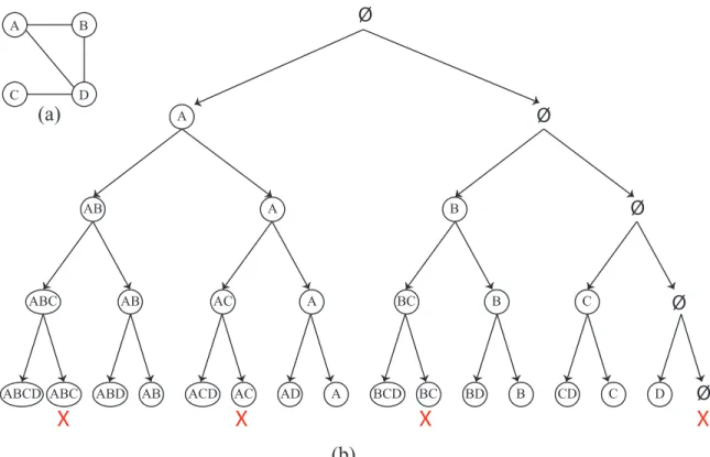
Figure 2.1. Traversal tree for generating all possible subsets of vertices and then checking the connectivity of each subset; Crossed out leaf nodes indicate unconnected subsets

A simple way to enumerate connected induced subgraphs of a graph G = (V, E) is to generate the power set P(V) of the vertex setV, and for each subset u ∈ P(V), we check if the vertices inu are connected or not.

To generate the power setP(V) of the vertex setV, we go for each vertex, one by one, and then either retain it or ignore it. We do this step recursively. Figure 2.1 (a) shows a sample graph of four vertices. Figure 2.1 (b) shows a binary tree that represents how the power set of the vertices is generated. The root has two children nodes, one has the avertex and the other one does not. Each of them has two children at depth = 1, one child that contains the b vertex and the other one does not. At depth = 2, each node has two children, one contains the c vertex and the other one does not. The same is done at depth = 3, but here we have one child node that contains thed

vertex and the other one does not. Finally, at depth = 4 we have the leaf nodes that represent the power set. At this point, we check the connectivity for each generated subset, and we exclude it if its vertices are not connected.

D B C A A B C D ABDC ABD AB BD CD BDC ADC AD

Ø

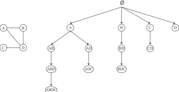
Figure 2.2. Traversal tree generated by Depth First Search approach to enumerate connected induced subgraphs

Algorithm 1 shows the pseudo-code. It’s clear that it takesO(2N) to enumerate all subsets, whereN =|V|, and for each subset, it takesO(N) to check the connectivity of the subset, hence, total time of this algorithm isO(N∗2N). Note that this is depth-first search algorithm and it uses a total extra memory of O(N).

2.1.2. Depth First Search Traversal (DFS)

Algorithm 2 Depth First Search Traversal

Input: G= (V, E): an undirected graph 1: visited={} 2: forv∈Cdo 3: EnumerateCIS({v},N eighbors{v}) 4: end for 5: 6: function_EnumerateCIS(U,C) 7: if U∈visitedthen 8: return 9: end if 10: output U 11: visited=visited∪U 12: forv∈C do 13: C0=N eighbors(U∪ {v}) 14: EnumerateCIS(U∪ {v},C0) 15: end for 16: end function

Another way to generate connected induced subgraphs is to only generate connected sub-graphs, by starting with one vertex as a subgraph (N = 1), and extending it with one of its direct neighbors to get a connected subgraph with sizeN+1, then we check if the subgraph was previously generated or not. The process of extending the subgraph with one neighbor at a time is continued until the extended subgraph is previously visited, or there are no more direct neighbors of the subgraph. An example of how this algorithm enumerates connected induced subgraphs is shown in Figure 2.2. We start with a subgraph that contains only the vertexA, mark the subgraph as visited, and then extending it with vertexB to get subgraphABwhich is also marked as visited. The same way is followed to generate subgraph ABD and ABDC. Then the algorithm extends subgraph A

with vertexD to generate subgraphAD and marks it as visited. Now it tries to extend AD with

B to get ADB, but does not complete the extension step since ABD was already discovered and marked as visited.

Algorithm 2 shows the pseudo-code. The algorithm stores all connected induced subgraphs is a shared memory (line 11). Since the number of connected induced subgraphs can be exponential, total space used by this algorithm is O(N ∗2N_).

Algorithm 3 Breadth First Search Traversal

Input: G= (V, E): an undirected graph 1: visited={} 2: 3: function_EnumerateCIS 4: queue={} 5: visited={} 6: forv∈V do 7: visited=visited∪ {v} 8: queue.enqueue({v}) 9: end for 10: whilequeue6=∅do 11: U =queue.dequeue() 12: output U 13: C=N eighbors(U) 14: forv∈C do 15: U0=U∪ {v} 16: if U06∈visitedthen 17: visited=visited∪U0 18: queue.enqueue(U0) 19: end if 20: end for

(a)

(b)

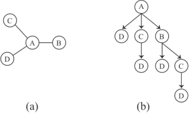
Figure 2.3. Creating a local search tree. (a) The input graph with an anchor vertex A. (b) Binomial tree to traverse all subgraphs induced by vertex A and its direct neighbors

2.1.3. Breadth First Search Traversal (BFS)

Breadth First Search Traversal is similar to Depth First Search Traversal in terms of mem-ory consumption and generating only connected subgraphs. Both require to store all discovered subgraphs in a shared memory, and for each generated subgraph they check if it has been previously discovered. The difference is the order in which the subgraphs are discovered. In Breadth First Search, all subgraphs with size = 1 are discovered first, and then subgraphs with size = 2, and so on, until the whole subgraph of sizeN is discovered.

Algorithm 3 shows the pseudo-code. The algorithm stores all connected induced subgraphs in a shared memory (lines 7 and 17). Since the number of connected induced subgraphs can be exponential, total space used by this algorithm isO(N ∗2N).

2.2. BDDE Algorithm

The BDDE algorithm follows a breadth-first discovery and depth-first extension approach to enumerate all connected induced subgraphs. For each vertex v ∈V, it builds an enumeration tree that is rooted atv, and each pathP(Kn) from the nodeKnto the rootvrepresents a unique connected vertex set U ⊆ V. After enumerating all connected vertex sets that include v, v is deleted from the graph G(V, E). The process is repeated for allv∈V untilV is empty.

2.2.1. Base Case

In this section, we focus on enumerating the subgraphs induced by a vertexv ∈V and its direct neighbors. Clearly, the direct neighbors of v can be treated as a set since any combination of them and the vertex v will induce a connected subgraph. Hence, a binomial tree [13] can be used to enumerate all these connected induced subgraphs. Binomial tree is a data structure that

(a)

(b)

Figure 2.4. Extending the local search node approach to enumerate subgraphs beyond the direct neighbors. (a) Building a binomial tree to traverse all subgraphs induced by vertex A and its direct neighbors. (b) Treating the subgraph ACD as a local search node and extending the binomial tree to traverse all subgraphs induced by vertex ACD and their direct neighbors

is used to enumerate all subsets of a set, and each node in the tree has children that are copies of all branches that are rooted at siblings that proceed the node in the tree.

Figure 2.3 (a) shows a sample graph with four vertices. Figure 2.3 (b) shows the binomial tree for enumerating all connected induced subgraphs that include vertex A. Each path from a node in the tree to the root r represents a connected induced subgraph.

This approach can be extended to enumerate subgraphs beyond the direct neighbors of a vertex, by following each path in the binomial tree and treating it as a local search node, and building a sub-binomial tree for the direct neighbors of all vertices in the path except the vertices that are already visited.

B C A G E A B C E C G E G C E C

Figure 2.5. The traversal tree built by the BDDE algorithm

Figure 2.4 shows how to extend this approach to enumerate subgraphs beyond the direct neighbors of a vertex.

2.2.2. Enumeration of All Connected Induced Subgraphs

The local search node approach can be combined with the depth-first approach to enumerate all subgraphs. Instead of using neighbors to build the tree, we use the branches generated by depth-first search. All neighbors of a local search tree are marked as visited before recursively call the depth-first search function, that eliminates duplicates that might be generated if the same neighbors are reached again by continued depth search. An example of the tree constructed by the BDDE algorithm is shown in Figure 2.5. For a complete graph, the BDDE algorithm could consume a total space ofO(2N−1), where N is the number of vertices in the input graph.

Algorithm 4 TGE Algorithm [22] 1: functionEnumerateCIS(G= (V, E),S,r) 2: output S

3: if d(r) = 0then

4: return

5: end if

6: choose a vertexvadjacent tor

7: _EnumerateCIS(G/(r, v),S∪ {v},r) 8: EnumerateCIS(G\v,S,r)

9: end function

2.3. TGE Algorithm

TGE algorithm is an efficient algorithm for enumeration in general. The author shows that the algorithm takes a constant amortized time per solution. Amortized analysis considers the worst

(a)

Ø

(b)

Figure 2.6. Traversal tree for the TGE algorithm

case run time per operation, not per the algorithm. Algorithm 4 shows the pseudo code for the TGE algorithm and figure 2.6 shows the traversal tree generated by the algorithm.

2.4. Reverse Search

In Reverse Search, a pattern extension rule defines how to generate child search nodes from a parent search node in the search space. The basic idea of reverse search is to arrange all solutions to be enumerated in a tree, rooted at an empty set node (canonical object), where each node in the tree appears only once under a specific parent node. In reverse search, a parent operation determines the unique parent node of a search node. This operation can be repeatedly applied on any two different nodes in the search tree until they reach a shared canonical node, the root of the

Ø

(a)

(b)

X

X

X

X

X

Figure 2.7. Traversal tree for the MST reverse search algorithm; Crossed out search nodes indicate invalid children

the parent-child operation, we build a tree-shaped traversal route on the set of connected vertex sets. We perform the depth-first search on the tree without having the tree in memory to enumerate all induced connected subgraphs.

2.4.1. MST Approach

Avis and Fukuda [3] proposed an algorithm to enumerate connected induced subgraphs. They define the parent operation as follows: letG(V, E) be a connected graph and let U ⊂V be a connected vertex set, then U −j is the parent of U, wherej is the smallest vertex in U such that

G(U −j) is connected.

In order to traverse all connected induced subgraphs using this approach, we start with a one vertex subgraph and try to extend it with one vertex at a time to produce a valid child subgraph. To check the validity of the generated child graph, we delete the smallest vertex that keeps it connected and then we check if it matches the parent subgraph.

For efficient implementation of this algorithm, the minimum spanning tree (MST) of a subgraph is used to define the child operation. Given a connected graph G(V, E), first step is to assign each edge e∈E a unique weight in range of 1 to |E|. Then the childoperation is defined as follows: let G(V, E) be a connected graph and let U ⊂ V be a connected vertex set, then

U∗ =U∪ {v}is a valid child of U if and only if:

1. The degree of the vertexv is the M ST(U∗) is 1; this means the newly added vertex is a leaf in the MST, and

2. The vertexv has the least index among all the vertices in M ST(U∗) which have a degree of 1.

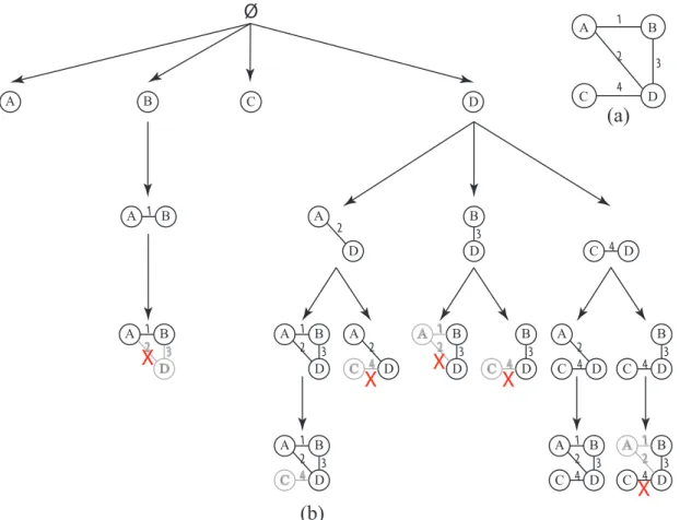
The time complexity for this algorithm isO(|V| ∗ |E|) for each connected induced subgraph. Figure 2.7 shows the traversal tree generated by the algorithm. Crossed out search nodes indicate invalid subgraphs.

3. A LINEAR DELAY LINEAR SPACE ALGORITHM FOR

ENUMERATION OF ALL CONNECTED INDUCED

SUBGRAPHS

3.1. Problem Description

Let G = (V, E) be an undirected graph, where V = {v1, ..., vn} is the set of vertices, and E ⊆ V ×V is the set of edges. For any vertex set U ⊆ V, let G(U) = (U, E(U)) denote the subgraph of Ginduced byU, whose edges include all the edges ofG with endpoints in U. We call

U a connected vertex set if G(U) is connected.

Problem Definition: Given an undirected graph G(V, E), enumerate all connected vertex sets,

CIS(G).

CIS(G) ={U|U ⊆V and G(U) is connected}

In this paper, we propose a linear-delay linear-space algorithm for enumerating all connected vertex sets of an undirected graph.

3.2. Parent Child Relationship The following lemma is essential:

Lemma 3.2.1. IfG(U) is a connected graph, s, u∈U are two distinct vertices, and uis the vertex

with the largest shortest path from s, then G(U −u) is connected.

Proof. Assume that u is the furthest vertex away from sand deleting u results in a disconnected

graph. This means that there exists at least one vertexu0 such that all paths between sand u0 go throughu. So, the shortest distance betweensandu0 is greater than the shortest distance between

sand u. This contradicts our assumption that uis the vertex with the longest shortest path from

sinG. Thus, G(U −u) is connected.

Clearly, we can choose any vertex in U, then find the furthest vertex away from it and delete it, and still get a connected subgraph with size |U| −1. It does not matter which vertex to choose, and also does not matter if the chosen vertex has many vertices with the same furthest distance because deleting any of them will produce a connected subgraph. In this work, for defining

A B C D E F A B C D E A B C D A B A

Ø

(a)

(b)

(c)

(d)

(e)

(f)

(g)

Figure 3.1. Repeatedly applying the parent operation on a graph. (a) The anchor vertex is A, and theutomst vertex is F. (b) After deleting vertex F, vertices C and E become the furthest vertices with the same distance away from A, so E is the utmostvertex. We reduce the subgraph by deleting vertex E. Then we keep applying the same operation until deleting the last vertex A a child/parent operation, we need to designate a vertex of the subgraph as the anchor vertex. We denote the vertex with the smallest vertex identifier (smallest vertex lexicographically) in U as

anchor(U). Let v ∈ U be the vertex with the longest shortest path to s = anchor(U). If there are more than one vertex with the longest shortest path, we take the one with the largest vertex identifier. We refer to the vertex with the longest shortest path to s in a graph (G(U)) as the

utmost vertex.

We define the parent graph for a subgraph as follows: Let G(U) be a connected induced subgraph,s=anchor(U), andv∈U is theutmostvertex, thenG(U−v) is the parent subgraph of

G(U) (lemma 3.2.1). Theparentoperation simply deletes theutmostvertex of a subgraph. It also can be repeatedly applied on a subgraph until reaching the canonical object (empty set). Figure 3.1 shows how to repeatedly apply the parentoperation on a graph until reaching the empty set.

Now we derive the the child operation from the parent operation, as follow: Let U be a connected vertex set,s=anchor(U),u∈U is the utmostvertex of U, and v∈V \U is connected to U. Then the subgraph induced by U∗ = U ∪ {v} is a child of G(U) if and only if v > s

(lexicographically) and one of the following conditions holds:

A B C D

Ø

X

X

X

X

X

X

X

X

(a)

(b)

X

X

X

X

X

X

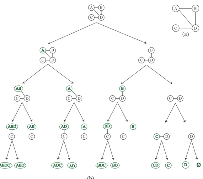
Figure 3.2. Enumeration tree of the sample graph; the crossed search nodes indicate invalid subgraphs

if G(U∗) is a valid child of G(U), we call v a valid candidate of G(U), otherwise, we call it an invalid candidate of G(U).

Figure 3.2 (a) shows a sample graph, and figure 3.2 (b) shows the enumeration tree of this graph. Every search node in the enumeration tree represents a connected induced subgraph. Figure 3.2 (b) shows that search node{A, D} is extended with vertexC to produce{A, D, C}; the other possibility{A, D, B}is crossed to indicate that it is not a valid child. In the leftmost branch, vertex

D cannot be added to search node {A, B, C} because distance(A, D) = 1< distance(A, C) = 2. Under the subtree rooted at B, vertex C cannot be added to {B, D} because distance(B, D) =

distance(B, C) = 1, but C is lexicographically less than D. In the middle, search node {B, A} is crossed out because vertex A is less than theanchor vertexB.

3.3. Distance-Array Representation

One way to speed up Reverse Search is to design a data structure that speeds up testing for valid children. In this section, we describe a data structure to represent each subgraph to be enumerated, such that checking each valid child takes a constant time. Moreover, building the data structure of a valid child, given the data structure of the parent node, takes only O(∆) where ∆ is the maximum degree of the input graph.

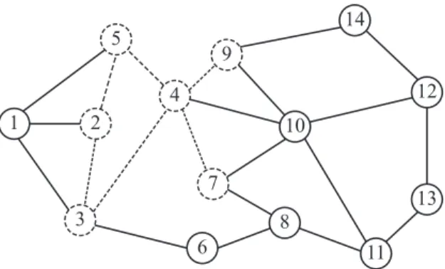
1 2 3 7 8 9 10 5 6 4 11 12 13 14

Figure 3.3. A sample graph of 14 vertices and 22 edges. The dashed edges and vertices show the subgraph induced by the vertex setU ={2,3,4,5,7,9}

Given a subgraph G = (V, E), we use a data structure of four arrays of size |V|. The U

array holds the vertices of the subgraph in the same order they were visited. The C array holds the neighbors (candidates) of the subgraph. The D array holds the distance between the anchor

vertex and all other vertices. And theP array keeps track of the parent of each vertex in U or in

C; The parent of a vertex v is the vertex connected to it on the path to the anchor when v was first added toC. Theanchor vertex does not have a parent vertex.

Figure 3.3 shows a sample graph G of 14 vertices and 22 edges. The dashed vertices and edges represent the subgraph induced by the subset U = {2,3,4,5,7,9}. Here is how the data structure would look like:

U 2 3 5 4 7 9

C 1 3 5 4 6 7 9 10 8 14

v 1 2 3 4 5 6 7 8 9 10 11 12 13 14

D[v] 1 0 1 2 1 2 3 4 3 3 - - - 4

P[v] 2 -1 2 3 2 3 4 7 4 4 - - - 9

The anchor vertex of the induced subgraph G(U) is 2, and the utmost vertex is 9, with distance 3 away from theanchorvertex. The whole graph has 14 vertices labeled from 1 to 14. Only 6 vertices belong to the subsetU and there are only five neighbors in C. Using this representation, we can easily determine the anchor vertex, since it is the first one in U, and the utmost vertex, since it is the last vertex inU. We can also get the distance between any neighbor of the subgraph

Using this representation, we can, for instance, extend the subgraph G(U) with the valid neighbor vertex v = 10 to form the subgraph induced by the subset U∗ ={2,3,4,5,7,9,10}. We need to add neighbors ofv= 10 toCarray and update their distances inDto be 4, and their parent inP to be 10. This will take only O(∆). The next tables show the data structure representation of U∗. U 2 3 5 4 7 9 10 C 1 3 5 4 6 7 9 10 8 14 11 12 v 1 2 3 4 5 6 7 8 9 10 11 12 13 14 D[v] 1 0 1 2 1 2 3 4 3 3 4 4 - 4 P[v] 2 -1 2 3 2 3 4 7 4 4 10 10 - 9

When backtracking, the P array is used to determine which candidates to be deleted from

C. For instance, when backtracking from U∗ to U, we first delete last added candidates whose parent is 10 from C (11 and 12) and reset the values of these indices in theD and P arrays, then we delete the 10 vertex from U.

3.4. Invalid Candidates Redundant Check

While analyzing the algorithm, we noticed that theC array holds many invalid candidates as the algorithm goes deep in the recursion, and the validity of each candidate is checked at each level of the recursion. This is time consuming and it decreases the efficiency of the algorithm. To overcome this issue, we remove the candidate from C once it becomes invalid, and we maintain three extra arrays to hold the invalid candidates and their information that are needed to insert them back into their original indices inC when backtracking. The three extra arrays are:

1. IC: The invalid candidates array

2. ICIV: The invalid candidates’ invalidity vertex 3. ICOI: The invalid candidates’ original indices inC

The invalidity vertex of a vertex v is the last added vertex toU whenv became invalid. When a candidate v in C becomes invalid, we first add it to the IC array and store its original index atC inICOI[v], then we store its invalidity vertex in ICIV[v], and finally we move

the right most vertex in C to the index of the deleted vertex. That guarantees a constant time checking and deletion for each invalid candidate. When backtracking, we just revert the procedure to get the original information before recursion.

We consider a candidate whose vertex identifier is smaller than the anchor vertex as a special case; we never add it into the C array.

For example, the subgraphU∗ ={2,3,4,5,7,9,10}mentioned in the previous section would be represented like: U 2 3 5 4 7 9 10 C 8 14 11 12 IC 6 v 1 2 3 4 5 6 7 8 9 10 11 12 13 14 D[v] - 0 1 2 1 2 3 4 3 3 4 4 - 4 P[v] - - 2 3 2 3 4 7 4 4 10 10 - 9 ICIV[v] - - - 7 - - - -ICOI[v] - - 1 2 1 1 2 - 1 2 - - -

-To extend it with the valid neighbor vertex v= 11, we do the following steps: 1. Move 11 fromU toC and setICOI[11] = 3 since 11 was at index 3 inC

2. Move the right most vertex inC (12) to the original place of 11 in C;C={8,14,12}

3. At this point, the candidate vertex 8 becomes invalid since it’s closer to the anchor vertex than theutmost vertex (11), hence, we move it to theIC array, and setICIV[8] = 11, then setICOI[8] = 1 since it was at index 1 inC, and finally, we move the right most vertex inC

(12) to the original place of 8;C ={12,14}

4. Add the new candidate 13 into C and set P[13] = 11 since 11 is the vertex connected to it on the path to theanchor vertex, and set D[13] =D[11] + 1 = 4; C={12,14,13}

After applying the previous steps, we get the following data structure, which represents the subgraph induced by the subset{2,3,4,5,7,9,10,11}:

U 2 3 5 4 7 9 10 11 C 12 14 13 IC 6 8 v 1 2 3 4 5 6 7 8 9 10 11 12 13 14 D[v] - 0 1 2 1 2 3 4 3 3 4 4 5 4 P[v] - - 2 3 2 3 4 7 4 4 10 10 11 9 ICIV[v] - - - 7 - 11 - - - -ICOI[v] - - 1 2 1 1 2 1 1 2 3 - -

-Note that applying the four steps in reverse order on this data structure produces the original data structure before extending it with the valid candidate (11). Moreover, applying them in reverse order recursively will produce the data structure of the anchor vertex only:

U 2 C 3 5 IC v 1 2 3 4 5 6 7 8 9 10 11 12 13 14 D[v] - 0 1 - 1 - - - -P[v] - - 2 - 2 - - - -ICIV[v] - - - -ICOI[v] - - - -3.5. Algorithm

Algorithm 5 shows pseudo-code for our algorithm. The recursive function takes a connected vertex set U and the set of candidate vertices. For each vertex v in the candidate set, it checks if it a valid extension and recursively calls the EnumerateCIS function. The algorithm invokes the

EnumerateCIS function for each vertex in the graph.

3.6. Complexity Analysis

An algorithm is said to be a linear-delay algorithm if it takes linear time, in terms of input size, to compute the next solution given a solution, or to detect that there are no more solutions. In our case, we consider the time the algorithm takes to generate the first child subgraph, given

Algorithm 5 Mining All Connected Induced Subgraphs Input: G= (V, E): an undirected graph 1: foru∈V do 2: EnumerateCIS({u},N eighbors({u})) 3: end for 4: 5: function_EnumerateCIS(U,C) 6: output U 7: forv∈C do 8: if isValidExtension(U,v)then 9: C0=N eighbors(U∪ {v}) 10: _EnumerateCIS(U∪ {v},C0) 11: end if 12: end for 13: end function 14: 15: functionisValidExtension(U,v) 16: s=anchor(U) 17: x=lastAdded(U) 18: if v < sthen 19: returnF alse 20: end if

21: if distance(s, v)> distance(s, x)then

22: returnT rue

23: end if

24: returndistance(s, v) =distance(s, x) andv > x

25: end function

the parent subgraph. Clearly, our algorithm checks if a vertex is a valid neighbor of a subgraph in a constant timeO(1) (Algorithm 5 line 8). It checks this condition for all vertices in the candidate set of a given connected vertex set. So, if there are no more solutions, the total delay is O(N) where N = |V|. In case there is a valid neighbor, the algorithm takes O(∆) time to update the arrays of the data structure.

Note that the algorithm is a Depth First Search (DFS) algorithm which ensures that the space used is bounded by the depth of the search tree. This depth is bounded by the number of vertices in the graph since at each level we add one vertex. So the depth is linear in the number of nodesN, and we use 7 arrays of size N to keep track of which vertices are in the search node, their neighbors, and their distances to theanchor vertex. So, the algorithm uses a total extra space of

AB 1,1,0,0,1 A 1,1,0,1,1 AF 0,1,0,0,1 AH 1,1,0,0,1 ABH 1,1,0,0,1 ABC 1,1,0,0,1 ABG 1,0,0,0,1 ABF 0,1,0,0,1

X

X

X

X

X

X

X

X

X

Figure 3.4. (a) An example node attributed graph. (b) A portion of the traverse tree for attributed graph in figure 3.4 with Smin= 2. Crossed search nodes indicate pruned children.

4. MAXIMAL COHESIVE SUBGRAPHS

In many applications, we are only interested in connected subgraphs that meet a user-defined constraint.

4.1. Problem Description

Let f : 2V → R denote a scoring function that quantifies vertex sets. Moreover, given a

thresholdδ, the anti-monotone constraint guarantees that if the score of a vertex set is at least δ, then score of each subset of the vertex set is also at leastδ, i.e.,f(U)≥δ =⇒ ∀U∗ _{⊂U :f(U}∗_)≥δ

In this section, we assume that the vertices in the graph are annotated with features. This leads to the undirected attributed graph G= (V, E, f) whereV is the set of vertices, E is the set of edges, andf :V → {0,1}d _{is a function that maps vertices tod-dimensional binary vectors. We}

are interested in mining subsets of connected vertices that have similar features. A dimension j is a cohesive dimension for a vertex set(subgraph) if the value of the dimension is ‘1’ in all the binary vectors of the vertices of the set; j is cohesive for U if ∀v∈U |f(v)[j] = 1. Let A(U) denote the set of cohesive dimensions for U.

Given a user-defined threshold Smin, a subgraph G(U) is called cohesive, if the number

of dimensions in A(U) is at least Smin. The cohesive condition is an anti-monotone constraint

where all the subgraphs of a cohesive graph are also cohesive. The set of all cohesive subgraphs for an attributed graph will have a large number of overlapping subgraphs since the subgraphs of a cohesive subgraph are also cohesive. To reduce redundancy in the output subgraphs, we require the subgraphs to be maximally cohesive. A subgraph is maximal cohesive subgraphif it does not have a supergraph that is cohesive, i.e.,G(U) ismaximal cohesive if@U∗ ⊃U, such that A(U∗)≥Smin.

Problem Definition: Given an attributed graphG= (V, E, f), and thresholdSmin, the problem

of mining the set of maximal cohesive subgraphsis to enumerate the set:

4.2. Approach

This problem can be addressed by employing the reverse search enumeration approach in algorithm 5 to enumerate all cohesive subgraphs and report only leaf search nodes that do not have any valid or invalid cohesive child nodes. For a highly-connected graph and a relaxed cohesive con-straint, enumerating the entire search tree of all cohesive subgraphs is computationally expensive. In the following section, we describe pruning strategies to reduce the size of the enumeration tree by pruning entire search branches without missing any search nodes. The pruning strategies result in significant performance improvement.

4.3. Pruning Strategies

4.3.1. Nodes with A Preceding Covering Sibling

Letx and ybe two neighbors ofG(U) such thatx is closer to anchor(U) thany (x≺U y),

andG(U∪ {x}) andG(U∪ {y}) are cohesive subgraphs withA(U∪ {y})⊆A(U∪ {x}), then none of them is a maximal cohesive subgraph, and any maximal subgraph that containsG(U∪ {x}) will also containG(U∪ {y}), and vise versa. Moreover,G(U∪ {x, y}) is also a cohesive subgraphs that can be reached from both G(U ∪ {x}) and G(U ∪ {y}), but is a valid child of only one of them. Note that sinceA(U∪ {y})⊆A(U∪ {x}), we get A(U∪ {x, y}) =A(U∪ {y}). In this case, we can prune the search branch rooted at one of the two subgraphs.

Lemma 4.3.1. Let G(U∪ {x})andG(U∪ {y}) be two cohesive subgraphs,xis closer toanchor(U)

than y (x≺_U y), and A(U∪ {y})⊆A(U ∪ {x}), then the search branch rooted at G(U ∪ {y}) can

be safely pruned.

Proof. For a set of vertices Z ⊆V \ {x∪y}, assume that G(U ∪ {y} ∪Z) is a maximal cohesive

subgraph. G(U ∪ {y} ∪ Z ∪x) is a cohesive subgraph since x is connected to U and can be added toG(U∪ {y} ∪Z) without violating the attribute similarity constraint. This contradicts our assumption thatG(U∪ {y} ∪Z) is a maximal cohesive subgraph. This proves thatG(U∪ {y} ∪Z) is not a maximal cohesive subgraph. Moreover,G(U∪ {y} ∪Z∪x) is not a descendant ofG(U∪ {y}) since x is not valid extension once y is added to vertex set U because x is closer to anchor(U) thany. So none of the descendants ofG(U∪ {y}) will be a maximal cohesive subgraph. Therefore, it is safe to prune the search branch rooted at G(U ∪ {y}) without losing any maximal cohesive subgraphs.

Figure 3.4 (a) shows a sample attributed subgraph, and Figure 3.4 (b) shows a portion of the enumeration tree of this graph with Smin = 2. Search node{A, F} is pruned because it has a preceding sibling {A, B} whereA({A, B, F}) =A({A, F}). Similarly, search nodes {A, B, C} and

{A, B, G} are also pruned because they have a preceding sibling{A, B, H}whereA({A, B, H, C}) =A({A, B, C}) and A({A, B, H, G}) =A({A, B, G}).

Level One Pruning: Pruning for level one (single vertex) is a special case, where U =∅ and

A(U) ={1}d_{. If a vertexx in level one has a preceding connected vertexy withA(y)⊆A(x), then} y can be safely pruned. In Figure 3.4, the search branch rooted atC can be safely pruned because it is connected toB and and A(C) ⊆A(B). Similarly, the branch rooted at H is pruned since H

is connected to A andA(H)⊆A(A).

4.3.2. Nodes with the Same Features as its Parent

This pruning strategy handles a special case where the attributes of a child node are identical to those of the parent node. After sorting neighbors of U, if there is a child U∗ such that A(U) = A(U∗), then all succeeding neighbors can be pruned safely using the previous lemma, because their descendants will be enumerated under theU∗ search branch. Although it looks like that this pruning operation is theoretically redundant of the first operation, it saves practically the time needed to check if the siblings are covered by any proceeding one. So once we observe that there is a node with the same feathers as the parent node, there is no need to check whether the succeeding neighbors are covered by this node. We will show in the experiments section that this pruning technique improves the performance.

In Figure 3.4 (b), search node {A, B, F, H} has same features as its parent, hence, all its succeeding siblings can be pruned.

4.4. Algorithm

Algorithm 6 shows the pseudo code for our algorithm. The recursive function builds an enumeration tree. The result of this algorithm is the set of all maximal cohesive subgraphs M. The main procedure is called for each cohesive vertex in the graph (lines 2-7). Sorting the neighbors according to the total order (closeness to U) is done in line 10. Checking for pruning the search node rooted atU∪ {vi}is done in 15-19. Pruning the succeeding neighboring search nodes is done

in lines 23-25. If there are no cohesive supergraphs of the current subgraph then it is added to the set of maximal subgraphs (lines 28-30).

Algorithm 6 Mining All Maximal Cohesive Subgraphs

Input:

G= (V, E, f): an undirected graph

Smin: minimum number of similar attributes per pattern

Output:

M: all maximal cohesive subgraphs 1: M={}

2: forall verticesvi∈V(G)do

3: U ← {vi} 4: if |A(U)| ≥Sminthen 5: MineMaximalCohesivePatterns(U) 6: end if 7: end for 8: function_{MineMaximalCohesivePatterns}(U) 9: locally maximal←true

10: Sort(N eighbors(U)) 11: forvi∈N eighbors(U)do

12: LetU0=U∪vi

13: if |A(U0)| ≥Sminthen

14: locally maximal←f alse

15: forvj∈N eighbors(U) andj < ido

16: if A(U0) =A(U0∪vj)then 17: Go to line 11 18: end if 19: end for 20: if _isChild(U0,U)then 21: MineMaximalCohesivePatterns(U0) 22: end if 23: if A(U0) =A(U)then 24: Break 25: end if 26: end if 27: end for

28: if locally maximalthen

29: M=M ∪U

30: end if

31: end function

5. EXPERIMENTAL RESULTS

We compare the performance of the proposed approach for enumerating all connected in-duced subgraphs to that of three existing algorithms on random graphs with varying graph size and density. Moreover, we test the running time on real enzymes. Moreover, to test the performance of the proposed approach for mining maximal cohesive subgraphs, we evaluate the performance on a real protein-protein interaction network with gene dysregulation profile in 13 cancer types as attributes. All experiments were performed on a machine with Intel Xeon 2.40GHz processor with 16 Gbytes main memory, running the Linux operating system. The two reverse search enumeration approaches were implemented in C++. The TGE algorithm is implemented in C and the BDDE algorithm in Perl as provided by their respective authors.

5.1. Performance on Random Graphs

We generated random graphs with varying numbers of nodes and density. Figure 5.1 shows the running times on graphs with varying size while keeping the density at 0.6. Figure 5.2 shows the running times on random graphs with varying density while the number of vertices was set to 27. We can see that RS-SP runs about one order of magnitude faster. We can see that our proposed algorithm is at least an order of magnitude faster than the best competing algorithm (TGE) and two orders of magnitude faster that the BDDE and RS-MST algorithms. For graphs with larger number of nodes (> 28), the BDDE algorithm uses too much memory and crashes after 1 hour. For larger graphs (>31), the RS-MST did not finish the enumeration task in 27 hours.

5.2. Performance on Real Data

We tested our algorithm on real chemical graphs downloaded from the network repository [18]. We compared against the TGE algorithm since it is the fastest among the competing algo-rithms. We ran both algorithms on ten graphs for which the running time is less than nine hours. For larger graphs, it takes days before we could get any results. Table 5.1 shows the running time of the TGE and RS-SP algorithms; RS-SP is several times faster than the TGE algorithm. Due to the nature of chemical compounds, most atoms (nodes) have a degree of at most 8 (maximal valence of atoms), and thus large chemical graphs are not dense. For these sparse graphs, the speedup is

1 10 100 1000 10000 100000 25 26 27 28 29 30 31 32 33 34 Graph Size RS-MST BDDE TGE RS-SP

Figure 5.1. Running time on random graphs with varying graph size; graph density set to 0.6

1 10 100 1000 10000 0.2 0.4 0.6 0.8 1

Running Time (in seconds)

Graph Density

RS-MST BDDE TGE RS-SP

Table 5.1. Running time on real enzyme graphs Graph ID |V| ρ |CIS(G)| T GE RS-SP (in millions) 502 36 0.116 53.4 10 1 522 37 0.123 2,376.7 438 54 31 38 0.115 4,470.0 850 119 108 38 0.117 3,125.8 566 69 23 39 0.109 713.7 111 15 274 40 0.094 1,723.2 291 45 303 41 0.101 22,534.5 4,935 696 513 41 0.112 31,041.1 5,017 715 530 42 0.096 44,684.8 7,510 1,117 500 43 0.109 184,636.9 31,130 4,618

5.3. Rejection Rate Analysis

In section 3.4, we show how to separate the invalid candadites of a subgraph in the enumer-ation tree into a separate array. We measure the effectiveness of this step by enumerating the con-nected induced subgraphs of random networks and counting how many times theisV alidExtension

function (Algorithm 5 line 8) was executed for checking invalid children. We had three different versions of the algorithm; First, we used the same data structure mentioned in section 3.3 where the C array contains all and subgraph’s vertices and neighbors (Version 1). Then we improved it by removing a candidate vertex from C once it’s added into U, and then pushing it back into its original index inC when backtracking (Version 2), and finally we implemented the data structure described in section 3.4 (Version 3). Table 5.2 shows the number of the connected induced sub-graphs of sub-graphs with varying size and constant density (0.6), along with the number of invalid checks performed when applying each version of the algorithm.

5.4. Cohesive Subnetworks

We use the BIOGRID protein-protein interaction network (version 3.4.160; May 2018) that has 287,970 interactions among 21,429 genes [4]. For attribute data, we used the gene dysregulation profile in 13 cancers. The dataset was generated from the gene and miRNA expression data of 13 tumor types and matched normal samples [12]. On average each cancer dataset had 2,380 dysregulated genes and each gene was dysregulated in 3.4 cancers. We ran the algorithm with all the pruning techniques on the attributed BIOGRID network for varying minimum support. The

Table 5.2. Rejection rate analysis on random graphs with varying size and constant density (0.6)

|V| |CIS| Invalid Candidates Count (in millions)

(in millions) Version 1 Version 2 Version 3

25 33.5 770.0 384.6 33.4 26 67.1 1,609.3 804.3 67.0 27 134.1 3,353.3 1,676.1 134.0 28 268.1 6,969.3 3,482.8 267.8 29 536.0 14,482.6 7,238.6 535.4 30 1,073.2 30,050.4 15,021.9 1,072.8 31 2,145.0 62,202.6 31,089.1 2,145.4 32 4,294.2 128,827.3 64,408.5 4,293.2 33 8,588.6 266,244.2 133,112.0 8,587.4 34 17,174.6 549,583.0 274,760.1 17,170.8

Table 5.3. Rejection rate analysis on random graphs with varying density and constant size (27)

ρ |CIS| Invalid Candidates Count (in millions)

(in millions) Version 1 Version 2 Version 3

0.2 57.4 1,402.4 621.5 49.1 0.4 129.9 3,243.5 1,606.7 127.4 0.6 134.1 3,353.3 1,676.1 134.0 0.8 134.2 3,355.4 1,677.7 134.2 1 134.2 3,355.4 1,677.7 134.2

algorithm was extremely fast finishing in less than one second forSmin ≥6, and for Smin= 2, and 1 it took 21 and 74 seconds, respectively.

5.5. Effectiveness of Pruning Techniques

To show the impact of the pruning techniques on the running time, we turned off the pruning techniques in the algorithm one at a time. Figure 5.3 shows the impact of the pruning techniques. For 1≤Smin ≥3, the algorithm without any pruning did not finish in 50 hours, resulting in more

than 400 speed up for each of the pruning techniques. 5.6. Maximal Cohesive Subgraph Analysis

Table 5.4 shows the topological properties and biological enrichment analysis for the re-ported maximal cohesive patterns. As we decrease Smin (relaxing the constraint), the average size of reported subgraphs, N, increases. Moreover, the number of subgraphs increases but then decreases whenSmin = 4 the subgraphs increase in size. We performed biological enrichment

anal-ysis of the reported patterns. We checked for enrichment (over-representation) of Gene Ontology (GO) biological process terms, KEGG pathways, and Disease Ontology (DO) terms. We used

50 100 150 200 250 300 350 400 1 2 3

Running Time (in seconds)

Minimum Support

Pruning Covered Pruning Succeeding All Pruning

Figure 5.3. Effectiveness of pruning techniques

the DAVID functional annotation tool for biological enrichment [10]. If a biological annotation is overrepresented in the reported subgraph’s genes, the subgraph is marked as enriched.

Table 5.4. Enrichment analysis of maximal cohesive subgraphs with different ontology databases

Smin N N Density KEGG% GO% DO%

1 28 798.6 0.185 68 82 71 2 260 124.5 0.19 54 59 64 3 642 58.5 0.147 56 69 68 4 816 43.5 0.123 61 77 75 5 705 37.0 0.106 72 83 77 6 429 31.2 0.104 77 87 81 7 183 25.9 0.113 82 90 79 8 72 20.7 0.125 81 92 78 9 32 15.3 0.154 69 91 72

Table 5.4 shows the percentage of patterns that are biologically enriched with different ontology databases. Some patterns are enriched with several terms and some terms are enriched in the genes of more than one pattern. Table 5.5 shows some of the KEGG pathways and diseases that were enriched the most in the reported patterns for Smin= 9.

Table 5.5. Top diseases and KEGG pathways enriched in the reported maximal cohesive sub-graphs;Smin = 9

Top 5 Diseases

DOID:3459 breast carcinoma

DOID:3908 non-small cell lung carcinoma DOID:3905 lung carcinoma

DOID:6050 esophageal disease DOID:2174 ocular cancer DOID:4231 histiocytoma DOID:10534 stomach cancer DOID:170 endocrine gland cancer

Top 5 KEGG pathways

hsa04110 Cell cycle hsa05166 HTLV-I infection hsa04218 Cellular senescence

hsa04914 Progesterone-mediated oocyte maturation hsa04114 Oocyte meiosis

6. CONCLUSION AND FUTURE WORK

In this thesis, we proposed an efficient algorithm for enumerating connected induced sub-graphs of an undirected graph. Building on that, we proposed an algorithm for mining all maximal cohesive subgraphs in a large network that integrates vertices’ attributes with subgraph enumera-tion. We also proposed two pruning techniques that remove futile search nodes in the enumeration tree, which lead to significant efficiency improvement. We demonstrated the effectiveness of both algorithms on synthetic and real datasets. On enumerating all connected induced subgraphs, our algorithm is several times faster than existing approaches. On dense graphs, the proposed approach is at least an order of magnitude faster than the best existing algorithm.

Experiments on real biological networks are done and we showed the effectiveness and efficiency of the algorithm achieve and the big improvement in performance. Biological enrichment analysis of the reported patterns shows that the patterns are biologically relevant and enriched with known biological processes and disease terms.

This thesis is addressing a fundamental problem and it has wider applicability and can benefit many existing algorithms that require subgraph enumeration. Future work will include developing an algorithm for mining maximal common subgraphs of multiple labeled graphs.

REFERENCES

[1] Comparison and enumeration of chemical graphs.Computational and Structural Biotechnology Journal, 5(6):e201302004, 2013.

[2] James Abello, Mauricio G. C. Resende, and Sandra Sudarsky. Massive quasi-clique detection.

InProceedings of the 5th Latin American Symposium on Theoretical Informatics, LATIN ’02,

pages 598–612, 2002.

[3] David Avis and Komei Fukuda. Reverse search for enumeration.Discrete Applied Mathematics, 65(1):21–46, 1996.

[4] Andrew Chatr-aryamontri et al. The biogrid interaction database: 2015 update. Nucleic acids research, 43(D1):D470–D478, 2015.

[5] Salim A Chowdhury, Rod K Nibbe, Mark R Chance, and Mehmet Koyut¨urk. Subnetwork state functions define dysregulated subnetworks in cancer. Journal of Computational Biology, 18(3):263–281, 2011.

[6] Han-Yu Chuang, Eunjung Lee, Yu-Tsueng Liu, Doheon Lee, and Trey Ideker. Network-based classification of breast cancer metastasis. Mol Syst Biol., 3:140, 2007.

[7] Han-Yu Chuang, Eunjung Lee, Yu-Tsueng Liu, Doheon Lee, and Trey Ideker. Network-based classification of breast cancer metastasis. Molecular systems biology, 3(1), 2007.

[8] K. J. Devlin. Fundamentals of Contemporary Set Theory. Universitext, 1979.

[9] Elisabeth Georgii, Sabine Dietmann, Takeaki Uno, Philipp Pagel, and Koji Tsuda. Enumer-ation of condition-dependent dense modules in protein interaction networks. Bioinformatics, 25(7):933–940, 2009.

[10] Da Wei Huang, Brad T. Sherman, and Richard A. Lempicki. Bioinformatics enrichment tools: paths toward the comprehensive functional analysis of large gene lists. Nucleic Acids Res., 37(1):1–13, 2009.

[11] Trey Ideker, Owen Ozier, Benno Schwikowski, and Andrew F. Siegel. Discovering regulatory and signalling circuits in molecular interaction networks.Bioinformatics, 18(Suppl 1):S233–40, 2002.

[12] Wei Jiang, Ramkrishna Mitra, Chen-Ching Lin, Quan Wang, Feixiong Cheng, and Zhongming Zhao. Systematic dissection of dysregulated transcription factor–mirna feed-forward loops across tumor types. Brief Bioinform., 17(6):996–1008, 2016.

[13] Donald E. Knuth. The Art of Computer Programming, volume 4A. Addison-Wesley, 2012. [14] H. Matsuda, T. Ishihara, and A. Hashimoto. Classifying molecular sequences using a linkage

graph with their pairwise similarities. Theor. Comput. Sci., 210(2):305–325, 1999.

[15] Sean Maxwell, Mark R Chance, and Mehmet Koyut¨urk. Efficiently enumerating all connected induced subgraphs of a large molecular network. InInternational Conference on Algorithms for Computational Biology, Lecture Notes in Computer Science, vol 8542, pages 171–182. Springer, Cham, 2014.

[16] Flavia Moser, Recep Colak, Arash Rafiey, and Martin Ester. Mining cohesive patterns from graphs with feature vectors. InSDM, volume 9, pages 593–604, 2009.

[17] Pierre-Nicolas Mougel, Christophe Rigotti, Marc Plantevit, and Olivier Gandrillon. Finding maximal homogeneous clique sets. Knowl. Inf. Syst., 39(3):579–608, June 2014.

[18] Ryan A. Rossi and Nesreen K. Ahmed. The network data repository with interactive graph analytics and visualization. InProceedings of the Twenty-Ninth AAAI Conference on Artificial Intelligence, 2015.

[19] Arlei Silva, Wagner Meira, Jr., and Mohammed J. Zaki. Mining attribute-structure correlated patterns in large attributed graphs. Proc. VLDB Endow., 5(5):466–477, 2012.

[20] Takeaki Uno. An efficient algorithm for enumerating pseudo cliques. In Proceedings of the 18th International Conference on Algorithms and Computation, ISAAC’07, pages 402–414. Springer-Verlag, 2007.

[21] Takeaki Uno. An efficient algorithm for solving pseudo clique enumeration problem. Algorith-mica, 56:3–16, 2010.

[22] Takeaki Uno. Constant time enumeration by amortization. InAlgorithms and Data Structures, pages 593–605. Springer International Publishing, 2015.