14
for Rendering
BO SUN Columbia University and RAVI RAMAMOORTHIUniversity of California, Berkeley
Many problems in computer graphics involve integrations of products of functions. Double- and triple-product integrals are commonly used in applications such as all-frequency relighting or importance sampling, but are limited to distant illumination. In contrast, near-field lighting from planar area lights involves an affine transform of the source radiance at different points in space. Our main contribution is a novel affine double- and triple-product integral theory; this generalization enables one of the product functions to be scaled and translated. We study the computational complexity in a number of bases, with particular attention to the common Haar wavelets. We show that while simple analytic formulae are not easily available, there is considerable sparsity that can be exploited computationally. We demonstrate a practical application to compute near-field lighting from planar area sources, that can be easily combined with most relighting algorithms. We also demonstrate initial results for wavelet importance sampling with near-field area lights, and image processing directly in the wavelet domain.
Categories and Subject Descriptors: G.1.0 [Numerical Analysis]: General; I.3.3 [Computer Graphics]: Picture/Image Generation; I.4.0 [Image Processing and Computer Vision]: General
General Terms: Algorithms, Theory
Additional Key Words and Phrases: Rendering, relighting, near-field illumination, image processing, importance sampling, wavelets, double and triple products ACM Reference Format:
Sun, B. and Ramamoorthi, R. 2009. Affine double- and triple-product wavelet integrals for rendering. ACM Trans. Graph. 28, 2, Article 14 (April 2009), 17 pages. DOI=10.1145/1516522.1516525 http://doi.acm.org/10.1145/1516522.1516525
1. INTRODUCTION
Integrations of products of functions are common in computer graphics and applied mathematics. For example, the reflection equa-tion can be viewed as either a triple-product integral [Ng et al. 2004] consisting of three factors: the lighting, BRDF, and visibility, or a double-product integral where the BRDF and visibility are com-bined into the light transport function. A common assumption is that the illumination is distant, and each factor is represented in basis functions such as spherical harmonics or wavelets.
Local area lights have long been used as not only a practical modeling tool, but also an indispensable artistic device to set up a mood for a scene, for example, comfortable couches in a living room illuminated by a ceiling lamp (Figure 1(a)), or stretch chairs
illumi-This work was supported in part by NSF grants (CCF 03-05322, 04-46916, 05-41259, 07-01775), a Sloan Research Fellowship, an ONR Young Investigator Award N00014-07-1-0900 and a Columbia University Presidential Fellowship, and by generous equipment and funding donations from NVIDIA, Intel and Adobe.
Author’s addresses: B. Sun, Department of Computer Science, Columbia University 450 Computer Science Building, 1214 Amsterdam Avenue, New York, NY 10027-7003; email: [email protected]; R. Ramamoorthi, Department of Electrical Engineering and Computer Science, University of California Berkeley, 627 Soda Hall, Berkeley, CA, 94720; email: [email protected].
Permission to make digital or hard copies of part or all of this work for personal or classroom use is granted without fee provided that copies are not made or distributed for profit or commercial advantage and that copies show this notice on the first page or initial screen of a display along with the full citation. Copyrights for components of this work owned by others than ACM must be honored. Abstracting with credit is permitted. To copy otherwise, to republish, to post on servers, to redistribute to lists, or to use any component of this work in other works requires prior specific permission and/or a fee. Permissions may be requested from Publications Dept., ACM, Inc., 2 Penn Plaza, Suite 701, New York, NY 10121-0701 USA, fax+1 (212) 869-0481, or [email protected].
c
2009 ACM 0730-0301/2009/04-ART14 $10.00
DOI 10.1145/1516522.1516525 http://doi.acm.org/10.1145/1516522.1516525
nated by the light from a circular light source (Figure 1(b)). Standard double- and triple-product integrals, however, are not suitable for near-field relighting. The basic problem is that the incident light-ing varies across the scene, and needs to be evaluated at all points in space. With proper parameterization, however, light propagation from planar area sources can be formulated as an affine transforma-tion of the original source radiance, as shown in Figure 1(c). We call the transformed integrals affine double- or triple-product integrals (Section 3).
We present the first theoretical and computational analysis of affine double- and triple-product integrals in computer graphics. For actual computations, we focus our analysis on Haar wavelets, which have gained considerable attention in relighting. Haar wavelets are simple, and superior in compactly representing all-frequency effects
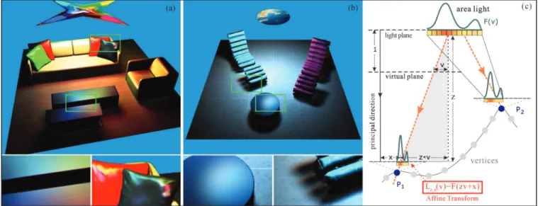
Fig. 1. (a) and (b): Our method enables relighting of scenes lit with near-field illumination. A planar area source can be moved, retextured, and reshaped at real-time rates. Important effects like spatially varying shading on the floors in 1(a) and 1(b), soft shadows under the chairs in the close-up of 1(b), and colored specularities on the cushions and tables in the close-ups of 1(a) and 1(b) are clearly visible. These effects are difficult to capture using only distant lighting, as shown in Figure 8(c). (c): Area lighting can be formulated as an affine transform. For simplicity, we parameterize the light field using a spatial coordinate xand an angular direction, given by the interceptvon a virtual plane, as shown in the diagram. The original area light is denoted asF(v), and the vertex’s incident radiance asLz,x(v), wherezandx, respectively, are the vertical and horizontal coordinates of the vertexP1. The intensity atP1,Lz,x(v), is then given
by an affine transform (F(zv+x)) from simple trigonometry. Our main contribution is a novel theory of affine double and triple product wavelet integrals that enables near-field area lighting to be used in almost any precomputation-based relighting framework.
such as natural lighting, specular BRDFs, and intricate shadowing, often using only 1 ∼ 2% of coefficients [Ng et al. 2003]. Our analysis approach can also be extended to non-Haar wavelets, as discussed briefly in Section 7. Fundamentally, the problem we are trying to solve is to find an efficient representation for wavelets that are affinely transformed (scaled and translated). Wavelets, however, are known for their lack of even translation invariance [Strang 1989]. For example, simply translating a Haar wavelet basis function one pixel to the left would change its coefficients dramatically, causing its power to spread across many different sub-bands.
Our main technical contribution is a novel affine double- and triple-product integral theory for Haar wavelets, which is presented in Section 4. The theory is developed primarily on 1D signals; since 2D and higher dimensional wavelets are simply products of 1D ba-sis functions, a direct extension to higher dimensions is possible (Section 4.4). Note that we focus on 1D affine transforms, namely, scaling and translations, and therefore do not consider general rota-tions and shears in 2D or 3D. As seen in our practical applicarota-tions, this provides a solid basis for a more general wavelet framework for many rendering problems. In Section 7, we also discuss extensions to non-Haar wavelets and nonlinear transformations.
The standard theory of double- and triple-product integrals is expressed in terms of standard coupling and tripling coefficients, respectively. Our theory studies the affine analogs, that must now account not only for the different basis functions being coupled or integrated, but also the scale and translation in the affine transform. Affine coupling and tripling coefficients therefore gain two more degrees of freedom and are, respectively, 4D and 5D functions for 1D signals. In Section 4.2, we show that these coefficients can be boiled down to an intuitive 2D analytic core function, which we call the canonical coupling coefficientM. The canonical coupling coef-ficient exposes the inherent sparsity of the affine transform, which
can be exploited to develop efficient computational methods. This is analogous to how standard tripling coefficients are theoretically complex, but actually sparse in Haar wavelets [Ng et al. 2004].
Our theoretical development enables fast practical algorithms for affine transforms in Haar wavelets. This overturns a commonly held view that operations like shifts or scales are difficult in the wavelet domain. One practical application of our theory is relighting, and we take a significant step towards generalizing wavelet-based relighting methods to near-field settings with planar area light sources (Section 5; Figures 1, 8, and 9). There are also applications to a variety of other problems that depend on wavelet representations. Section 6 describes initial solutions for wavelet importance sampling [Clarberg et al. 2005] with near-field area lights, and image processing (dilation and translation) directly in the wavelet domain. Section 7 briefly discusses extensions to non-Haar wavelets and nonlinear transformations, and addresses relighting with out-of-plane rotation and arbitrarily shaped 3D lights. Readers more interested in implementation may want to first familiarize themselves with the basic concepts introduced in Section 3, and then focus on the applications in Sections 5 and 6, skimming through the development of the theory in Section 4 as needed. 2. PREVIOUS WORK
Light transport analysis. Recent papers [Durand et al. 2005; Ramamoorthi et al. 2007] have conducted a comprehensive analysis of light transport in Fourier and gradient representations. As noted in Durand et al. [2005], one of the main aspects is the propagation of light from an area source, which can be written as an affine transform (in much the same form as Figure 1(c)). Ramamoorthi et al. [2007] characterized the basic mathematical operations of light transport, noting that linear or affine transforms are a key element, but there is
no simple formula in wavelets. By developing a framework for affine double- and triple-product wavelet integrals, we take a significant step towards a full computational framework for rendering in the wavelet domain.
Double and triple product integrals. Much of the work in relighting [Sloan et al. 2002; Ng et al. 2003] can be seen as double product integrals of the illumination and the light transport function. These integrals usually reduce to simple dot products in orthonormal bases like spherical harmonics and Haar wavelets. Subsequently, Ng et al. [2004] developed the triple-product integral framework to con-sider the integration of the lighting, BRDF, and visibility, as needed for changing both view and illumination. The same mathematics can be applied to efficiently multiplying two wavelet signals [Beylkin 1992a]. Most recently, these results have been generalized to prod-ucts of multiple functions [Sun and Mukherjee 2006]. Our work can be viewed as an important generalization of thestandard double-and triple-product integral framework toaffinedouble- and triple-product integrals. We also briefly discuss nonlinear transformations in Section 7.
Affine transforms of basis functions. Affine transforms of Fourier basis functions are well known [Bracewell et al. 1993]. Spherical harmonics can be analytically rotated, as often used for environment maps [Sloan et al. 2002]. However, the standard affine transform usually considered in the spatial domain has no simple analog in the spherical domain; therefore, we do not consider spher-ical harmonics in this article. Researchers have approximated the affine transform using a combination of spherical rotations and a spherical scaling operation [Wang et al. 2006a]. This approxima-tion is limited to only midrange illuminaapproxima-tion, since the distorapproxima-tion tends to be too severe in the near field.
Wavelets lack translation invariance, and have no simple formula for affine transforms. Beylkin [1992b] and others have studied the concurrent wavelet decomposition of all integer (not continuous) circulant shifts of a signal. In comparison, our goals are different and more ambitious in that we want to consider a general continuous affine transform (and not just all integer shifts). Nevertheless, we are inspired by the sparsity indicated by Beylkin [1992b] and Wang et al. [2006b] who studied wavelet rotations. We have developed a fast algorithm for wavelet affine transforms, even when no simple analytic formula exists.
Near field relighting and image processing. Relighting tech-niques have been developed from the basic approach introduced by Nimeroff et al. [1994] and Dorsey et al. [1995] to much recent work on Precomputed Radiance Transfer (PRT) [Sloan et al. 2002]. In terms of our application, the most closely related works are meth-ods extending PRT to near-field and dynamic settings. Spherical har-monic gradients [Annen et al. 2004] and scaling [Wang et al. 2006a] try to approximate the effects of midrange illumination. Spherical harmonic exponentiation [Ren et al. 2006] can render near-field soft shadowing effects in real time, but has to use sphere sets to approximate geometries so that affine transforms are avoided. As a precursor, Mei et al. [2004] proposed decomposing the illumination into directional lights and searching through precomputed spherical radiance transport maps to render dynamic scenes. Zhou et al. [2005] then developed precomputed shadow or source radiance fields1to
support all-frequency effects, but this cannot support very high
sam-1The radiance function of Zhou et al. is 5D, consisting of all possible spatial
locations and angular directions. This is just the light field from the source, and a simpler 4D representation, including possibly directly in the wavelet domain, should be possible. However, the 4D representation is very difficult
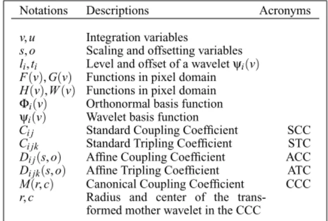
Notations Descriptions Acronyms
v,u Integration variables
s,o Scaling and offsetting variables
li,ti Level and offset of a waveletψi(v)
F(v),G(v) Functions in pixel domain
H(v),W(v) Functions in pixel domain
Φi(v) Orthonormal basis function
ψi(v) Wavelet basis function
Ci j Standard Coupling Coefficient SCC
Ci jk Standard Tripling Coefficient STC
Di j(s,o) Affine Coupling Coefficient ACC
Di jk(s,o) Affine Tripling Coefficient ATC
M(r,c) Canonical Coupling Coefficient CCC
r,c Radius and center of the trans-formed mother wavelet in the CCC Fig. 2. Notations used in the article.
pling rates nor general changes in the lighting (such as editing the pattern of an area source in lighting design). Kristensen et al. [2005] also extend PRT to local lighting using unstructured light clouds. Overall, these methods have to assume predetermined lights, allow-ing changes of only light positions or scale intensities. In contrast, our method first assumes planar area sources, allowing near-field re-lighting with dynamic editable lights, and eliminating the need for lighting-dependent precomputations and storage. In Section 7, we discuss a possible extension of our algorithm to general out-of-plane rotation and arbitrarily shaped 3D lights.
Other applications shown at the end of the article include wavelet importance sampling the product of the area lighting and general BRDFs for Monte Carlo offline rendering systems, which has previ-ously only been applied to distant environment maps [Clarberg et al. 2005]. In addition, we also explore image processing. A number of image operations such as additions and multiplications can already be performed directly in the wavelet domain [Drori and Lischinski 2003; Kutil 2005]. Our algorithms extend these operations to dilations and translations, which can be cast as affine transforms. 3. AFFINE DOUBLE AND TRIPLE PRODUCT
INTEGRALS
In this section, we introduce affine coupling and tripling coefficients. We use 1D wavelets for simplicity in our analysis (we will see that our results extend directly to higher dimensions in Section 4.4). Notation used in this article is shown in Figure 2.
3.1 Standard Coupling and Tripling Coefficients Double- and triple-product integrals can be written respectively as
H(v) = F(v)G(v)dv, (1) H(v) = F(v)G(v)W(v)dv, (2)
whereH,F,G, andW are functions in the spatial or angular do-main. For example, in relighting applications,vcould be the inci-dent angle, H could be the reflected radiance, and F,G, andW to unpack in real time for relighting applications that may require the full incident illumination field at any given pixel. By directly propagating lighting from the area light source, we bypass the need for these higher-dimensional representations.
could correspond to the lighting, visibility, and BRDF, respectively. For compact representation, it is common to expand them in basis functions. The double-product integral becomes
H(v) = i Fii(v) j Gjj(v) dv = i j FiGj i(v)j(v)dv = i j FiGjCi j, (3) Ci j = i(v)j(v)dv, (4)
where(v) are some set of orthonormal basis functions. We denote
Ci jas theStandard Coupling Coefficient, or SCC.
Similarly, the triple-product integral becomes
H(v) = i Fii(v) j Gjj(v) k Wkk(v) dv = i j k FiGjWk i(v)j(v)k(v)dv = i j k FiGjWkCi jk, (5) Ci jk = i(v)j(v)k(v)dv. (6)
We denoteCi jkas theStandard Tripling Coefficient, or STC.
3.2 Affine Coupling and Tripling Coefficients
The SCC and STC only apply well to functions that are “fixed” and “static.” We now consider functions that are affinely transformed. Without loss of generality, we assumeF(v) is scaled and translated to F(sv+o). With respect to the illustration in Figure 1(c), the offsetocorresponds to the horizontal positionx, and the scalesto the vertical distancez. This leads to an important variation of the standard product integral, which we call the affine double-product integral: H(s,o;v) = F(sv+o)G(v)dv = i Fii(sv+o) j Gjj(v) dv = i j FiGjDi j(s,o), (7) Di j(s,o)= i(sv+o)j(v)dv. (8)
We denoteDi j(s,o) as theAffine Coupling Coefficient, or ACC.
Just as standard triple-product integrals are used for multiplication, the same machinery as Eq. 8 is useful for affinely transforming a function. In fact, Eq. 7 is equivalent to an affine transform of F
followed by a standard double-product integral withG.
Similarly, the affine triple-product integral can be written as
H(s,o;v)= F(sv+o)G(v)W(v)dv = i Fii(sv+o) j Gjj(v) k Wkk(v) dv = i j k FiGjWkDi jk(s,o), (9) Di jk(s,o)= i(sv+o)j(v)k(v)dv. (10)
We denoteDi jk(s,o) as theAffine Tripling Coefficient, or ATC.
3.3 Discussion of Properties
Properties of SCC and STC. Because of the orthonormal re-lation between two different basis functions, the SCC reduces to a Kronecker delta function,Ci j = δi j, and has exactly Nnonzero
terms, whereNis the total number of basis functions. The STC is slightly more complicated. For general orthonormal bases, the com-plexity (i.e., number of nonzero coefficients) of the STC isO(N3).
Sparsity exists for bases with special structures [Ng et al. 2004], for example, the complexity isO(N) for pixel bases,O(N2) for 2D
Fourier series, andO(NlogN) for Haar wavelets. The complexities of the SCC and STC are recapped in Section 4.3. In addition, note that both the SCC and STC are symmetric. We have
Ci j =Cji, Ci jk=Cperm(i jk), (11)
whereperm(ijk) is any permutation of the triplet (i,j,k).
Properties of ACC and ATC. By contrast, the ACC and ATC both gain two more degrees of freedom, since there are two new arguments: the scalesand the offseto. In fact, the SCC and STC are special cases of the ACC and ATC, when the scale is 1 and the offset is 0.
Ci j =Di j(1,0), Cijk= Dijk(1,0) (12)
The ACC and ATC do not preserve the same symmetries of the SCC and STC. For example, the ACC follows this more complex identity.
Dij(s,o)= 1 sDji 1 s − o s . (13)
Relation between ACC and ATC.
LEMMA 1. For any orthonormal basis, the ATC can be
repre-sented using the the ACC and STC as Dijk(s,o)=
l
Dil(s,o)Cljk. (14)
The proof is in Appendix A, and follows from expanding
(sv+o) in terms of(v) and then using associativity. Lemma 1 indicates that the computational complexity of the affine tripling coefficientDi jk(s,o) relies on those of the ACC and STC. Lemma 1
also suggests a way of evaluating the ATC using the ACC and STC. 4. COMPLEXITY OF AFFINE COUPLING AND
TRIPLING COEFFICIENTS (ACC & ATC)
In this section, we study the computational complexity of the affine coupling and tripling coefficients (ACC and ATC), determining their numbers of nonzero terms in a number of bases. In wavelets, we fo-cus on the Haar basis for its simplicity. We present the main results
that are essential for understanding the key insights and implement-ing the theory, leavimplement-ing many detailed mathematical derivations for the appendices.
4.1 General, Pixel, and Fourier Bases
In general orthonormal bases, the complexities of the ACC and ATC are O(N2) andO(N3), respectively (they can be lower for some
values ofsando). This can be contrasted to the linear complexity of the SCC, and highlights the fact that the original orthonormal relation between different basis functions no longer holds under an affine transform.
Pixel basis functions, in mathematical terms, are disjoint and dis-crete step functions. A unique aspect of the pixel basis is that both the integration and product of multipledifferentpixels is zero. This leads directly to the linearO(N) complexity of the ACC and ATC. A detailed account of the complexity analysis is in Appendix B. De-spite its simplicity, the pixel basis is a poor basis for compression, which often outweighs its efficiency in calculation.
The Fourier series is mostly preferred in theoretical analysis and has a well-known 2D affine theorem [Bracewell et al. 1993]. Adapt-ing this theory to 1D (Appendix B), we show that the ACC in the Fourier basis can be mapped to the SCC, and thus has the same lin-ear O(N) complexity. The specific mapping depends on the scale
sand offseto. Similarly, the complexity of the ATC in the Fourier basis can be determined asO(N2) using Lemma 1 (Appendix B).
Spherical harmonics are the extension of the Fourier basis to the sphere. They are not considered in this discussion, since no standard operation in the spherical domain directly maps to the affine transform.
4.2 Haar Wavelets
We present our main theoretical contribution in this section, deriving the complexities of affine coupling and tripling coefficients in Haar wavelets. Readers interested in implementation may wish to skip to the summary of complexities in Section 4.3 on a first reading.
4.2.1 Wavelet and Scaling Functions. The normalized 1D Haar basis [Stollnitz et al. 1996] is defined as
—The mother scaling and wavelet functions are
φ(v)= 1, for 0≤v <1 0, otherwise, and ψ(v)= ⎧ ⎨ ⎩ 1, for 0≤v <1/2 −1, for 1/2≤v <1 0, otherwise.
—A normalized wavelet basisψj(v) at levellj and offsettj is ψj(v) = 2lj/2ψ(2ljv−tj),
which is a scaled and dilated copy of the mother wavelet. 4.2.2 Haar Canonical Coupling Coefficient (CCC). The ACC is a 4D function of the two subscriptsi and j, the scale s, and the offseto. Similarly, the ATC is a 5D function. Since accord-ing to Lemma 1 the ATC can be reduced to the ACC, we first fo-cus our analysis on the ACC. To reduce the dimensionality of the ACC, we invoke the standard property of Haar wavelets as a multi-resolution series and write wavelet basis functions in terms of the
mother waveletψ(v). Dij(s,o) = ψi(sv+o)ψj(v)dv = 2li+2l j ψ(2lisv−t i+2lio)ψ(2ljv−tj)dv (15)
To simplify Eq. (15), we make the substitutionu=2ljv−t
jso that
transformations of the two mother wavelets can be merged into a single combined transformation. We have
Di j(s,o) = 2 li−l j 2 ψ(2li−ljsu−t i +2lio+stj2li−lj)ψ(u)du = 2li−2l j ψ u 2r − c 2r + 1 2 ψ(u)du Di j(s,o) = 2 li−l j 2 M(r,c) , (16) where M(r,c)= ψ u 2r − c 2r + 1 2 ψ(u)du , (17) r= 2 lj−li−1 s , and c= 2lj−lit i−2ljo+2lj−li−1 s −tj. (18)
We callM(r,c) theCanonical Coupling Coefficient, or CCC. The CCC encapsulates the core structure of the ACC. Variablesr and
cdictate the combined transformation in waveletψ(u
2r −
c
2r +
1 2).
Intuitively, they are, respectively, theradiusandcenterof the trans-formed waveletψ(u
2r −
c
2r +
1
2), as shown in Figure 3(a).
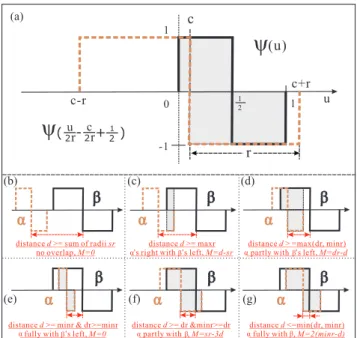
Property 1. The evaluation of the 4D affine coupling coefficient reduces to a combination of a few simple function computations and an estimate of the 2D analytic functionM(r,c) called the canonical coupling coefficient, as described by Eq. 16. Variablesr andcare given by Eq. 18.M(r,c) is a sparse, piecewise linear, and symmetric function.
In its analytic form,M(r,c) is a branching function as shown in Figure 4. The calculation of M(r,c) is equivalent to determining the overlapping relation between the original mother waveletψ(u) (denoted asβ) and the transformed oneψ(2ur − 2cr +12) (denoted asα). Their overlapping relation depends on theirrelativepositions (centers) and sizes (radii). We group their overlapping relations into six cases and show them in Figure 3. For brevity in exposition, we assume thatα’s radius is smaller than that ofβ, andαis located on the left. Our analysis will still hold whenα’s radius is actually larger or it is located on the right, sinceβcan then be viewed as “the transformed wavelet” and exchange roles withα. In all cases,
M(r,c) can be computed in no more than 9 lines of code (Figure 4 also cross-references the six cases in Figure 3).
4.2.3 Properties of Haar CCC. M(r,c) has special structures and important properties that can be exploited for computation. In Figure 5, we plot M(r,c) in bothr and c dimensions to better expose many such properties. We examine a few important ones here:
Sparsity. M(r,c) is sparse. As shown in Figure 5, M(r,c) is nonzero over only very limited ranges of the radiusr and the cen-terc. In particular,M(r,c) is zero when the right endpoint of the transformed wavelet is less than 0 (meaningc+r<0), or the left endpoint is greater than 1 (meaningc−r>1). In these cases, the
(a)
(b) (c) (d)
(e) (f) (g)
Fig. 3. The canonical coupling coefficientM(r,c) is an integration of two wavelets denoted asαandβ, withαbeing affinely transformed, as shown in (a). Variablesrandccorrespond to the radius and center of the transformed waveletα. (b)–(g) show different overlapping relations of waveletsαand β. Variablesmaxrandminrare, respectively, the bigger and smaller of the radii of the two wavelets, andsranddrtheir sum and difference. The red arrows show the distanced.
two wavelets do not overlap and their integration is 0. These two boundary conditions compactly combine to|c−0.5|>r+0.5.
M(r,c)=0, when|c−0.5|>r+0.5 (19) Since the ACC reduces to the CCC, the ACC will be sparse if many combinations ofi,j,s, andomakerandcfall into the zero ranges. We will discuss the complexity of the ACC formally in Section 4.2.4.
Piecewise linearity. M(r,c) is a piecewise linear function. As depicted in Figure 5,M(r,c) has only a limited set of slopes
{0,±1,±2±3}in bothr andcdimensions. This is because the partial derivatives ofM(r,c) with respect torandcare just combi-nations of a few mother waveletsψ(u). These mother wavelets are valued at three break-points (c−r,c+randc, as in Figure 3(a)) of the transformed waveletψ(u
2r −
c
2r +
1
2). The derivation of the
partial derivatives is in Appendix C. ∂M(r,c)
∂c =2ψ(c)−ψ(c−r)−ψ(c+r)= {0,±1,±2,±3}, (20)
∂M(r,c)
∂r =ψ(c−r)−ψ(c+r) = {0,±1,±2} (21)
Consequently, the ACC is also piecewise linear, and its gradient is easily computed from that ofM(r,c) using the chain rule.
Symmetry. M(r,c) is symmetric. In thecdimension, as shown in Figure 5(a),M(r,c) is reflection symmetric about 0.5. This reflec-tion symmetry is also used in computareflec-tion in Figure 4 as the calcu-lation depends not oncdirectly, but ond= |c−0.5|.d= |c−0.5| is reflection symmetric about 0.5. In mathematical terms, we have
M(r,0.5+c) = M(r,0.5−c). (22)
In therdimension,M(r,c) also has a certain degree of symmetry. Whenris above 1, we can invert its value to below 1 by changing
//candrare respectively the center and radius of the transformed wavelet. //dis the distance between the centers of the two wavelets.
//sranddrare respectively the sum and difference between the two radii.
1. d= |c 0.5|; sr=r+ 0.5; dr= |r 0.5|;
2. maxr=max(r, 0.5); minr=min(r, 0.5);
3. if (d> =sr) M= 0; // Fig. 3B
4. else if (d> =maxr) M=d sr; // Fig. 3C
5. else if (d> =max(dr,minr)) M=dr d; // Fig. 3D
6. else if (d> =min(dr,minr))
7. if (dr> =minr) M= 0; // Fig. 3E
8. else M=sr 3d; // Fig. 3F
9. else if (d< =min(dr,minr)) M= 2(minr d); // Fig. 3G Fig. 4. Analytic formula ofM(r,c) in pseudocode. Branches correspond to different overlappings between the two wavelets, as illustrated in Figure 3.
the integration variable in Eq. (16) tow= u
2r − c 2r + 1 2. M(r,c) = 2r M 1 4r, 1 2+ 1 4r − c 2r (23) Derivations of these symmetry properties are in Appendix C. Due to these symmetries, we only store a nonrepeating quarter ([0<r ≤1,−r ≤c≤0.5]) of the nonzero range of M(r,c) and save three-fourths of the storage space.
Boundedness. M(r,c) is both upper and lower bounded, which makes it ideal for quantization and encoding in hardware textures.
maxM(r,c) = 2min(r,0.5) ≤ 1,
minM(r,c) = −min(r,0.5) ≥ −0.5
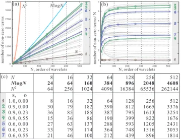
4.2.4 Complexities of Haar ACC and ATC. The number of nonzero ACC terms varies significantly with the scale and offset. We first show empirically in Figure 6 theO(NlogN) complexity of the ACC in Haar wavelets. Complexities for general wavelets are discussed in Section 7, and are found to be similar to the Haar case. In Figure 6(a), we plot the numbers of nonzero ACC terms versus the total numbers of the wavelets for 50 randomly generated sets of scales and offsets. Seven representative curves out of the 50 are highlighted, and their numerical values are tabulated in Figure 6(c). To better illustrate the logarithmic behavior part of theO(NlogN) complexity, we divide all curves byNand plot them again in Fig-ure 6(b). Note thatO(NlogN) is just an upper bound. The actual complexity of the ACC is comparable to that of standard tripling coefficients (STCs) developed by Ng et al. [2004]. TheO(NlogN) complexity can also be mathematically proved by determining the upper bound of the total overlapping pairs between the two wavelet trees, one of which is affinely transformed. We give the detailed proof in Appendix D. In practice, indices of nonzero ACC terms can be picked either using Eq. (19) (the sparsity property of the CCC), or from a compact pretabulated table, as implemented in Section 5.3.2. To compute the complexity of Haar ATC, we invoke the standard property of Haar wavelets that the product of two wavelets is either the finer wavelet up to a scale if they overlap, or zero otherwise. Therefore when wavelets overlap, the ATC reduces to the ACC, and subsequently to the CCC according to Property 1. When wavelets do not overlap, the ATC is simply zero. Based on this key observation, we derive Property 2 that relates the ATC to the CCC.
Property 2. The Haar ATC, as defined in Eq. (10), is evaluated using the canonical coupling coefficient as follows.
r-0.5 0.5-r 5 . 0 5 . 0 -5 . 0 5 . 0 - -1 1 -0.5 0.5 -r r -0.5-r 0.5+r 0.5-r r-0.5 r + 5 . 0 r -5 . 0 --1 1 3 2 -2 -3 -1 1 -1 3 -3 1 -1 1 3 2 -2 -3 -1 1 -0.5 -r -0.5 r 0.5 0.5 -r r -0.5-r 0.5-r r-0.5 0.5+r -1 1 2 -2 -1 1 -1 1 2 -2 1 -1 0.5 0 0c-0.5 1-c c 0 0.25 0.75 0 1-c c c-0.5 0.5 1 1 2 2-2c 3-4c 0.5 0 0.5 1.5-2c 2-2c 2 1 1 -1 1 -1 1 M M M M M c c c c c M M M M M r r r r r (a) (b)
Fig. 5. (a) Canonical Coupling CoefficientM(r,c) in thecdimension (the horizontal axis isc−0.5 to better demonstrate the symmetry) for all different ranges of the radiusr. The red labels represent line slopes, while the black labels are measurement marks along the axes; (b)M(r,c) in therdimension forc≥0.5. The horizontal axis is the radiusrof the transformed wavelet. Whenc≤0.5,M(r,c) can be computed using the symmetryM(r,c−0.5)=M(r,0.5−c). This graph illustrates a number of important properties ofM, such as its sparsity, piecewise linearity, symmetries, and boundedness.
N N NlogN , s o 8 64 8 30 36 15 27 33 21 24 16 256 16 79 85 36 63 79 46 64 32 1024 32 182 185 86 137 174 100 160 64 4096 64 390 387 190 288 364 212 384 128 16384 128 812 795 399 593 748 439 896 256 65536 256 1665 1613 822 1205 1516 896 2048 512 262144 512 3376 3254 1676 2431 3053 1814 4608 2 0 100 200 300 400 500 0 500 1000 1500 2000 2500 3000 3500 u nb m oz -n 0 100 200 300 1 2 3 4 5 6 7 n b m u o z-n 400 N2 N 500 NlogN (c) (a) (b)
Fig. 6. Complexity of affine Haar wavelet coupling coefficients for 50 randomly generated sets of scales and offsets. Figure 6(a) empirically shows theO(NlogN) complexity of the ACC. Seven representative curves out of 50 are highlighted and their values listed in Table (c). Note that in Figure 6(a) for most scales and offsets, the actual numbers of nonzero ACC terms fall well belowNlogN(cyan line), and some even belowN(when significant offsets and scales transform a large portion of the wavelet tree out of [0,1]). The formal proof of the complexity of the ACC is in Appendix D.
—In Eq. (10), if basis functionsj(v) andk(v) overlap, Di jk(s,o)=2
li−lm+ln
2 M(r,c), (24)
wheren=min(j,k),m=max(j,k), and
c = 2 lm−lit i−2lmo+2lm−li−1 s −tm, r = 2 lm−li−1 s . —Otherwise,Di jk(s,o)=0.
It can be shown that the complexity of the ATC in the Haar basis isO(Nlog2N). We leave the proof in Appendix D. For interested
readers, Property 2 can also be verified using Lemma 1. 4.3 Summary of Complexities in All Bases
The following table summarizes the computational complexities of the SCC, STC, ACC, and ATC in different bases. For general orthonormal bases, there is no sparsity due to the lack of special structures. The pixel basis, despite its simplicity, is a poor basis for compression and hence undesirable for practical applications. The Fourier basis is widely used in theoretical analysis, but is not good at capturing all-frequency lighting (or visibility/BRDF) as shown in Ng et al. [2003]. Haar wavelets are preferred in all-frequency relighting and only need a handful of coefficients and basis func-tions to achieve good approximafunc-tions. To distinguish fromN, the total number of basis functions, we denote the number of terms re-tained after compression asn.nis usually around 1 ∼ 2% ofN
for wavelets. As shown in the following table, Haar wavelets have linear or close-to-linear complexities ranging fromntoO(nlog2N) across all columns. In practice, we would need to compute far fewer terms after compression than in the other bases. This makes Haar wavelets ideal for many operations in practical applications. We also show the complexities of ACCs and ATCs for general wavelets are
O(nlogN) andO(nlog2N), respectively, in Section 7.
Bases SCC ACC STC ATC
General N O(N2) O(N3) O(N3)
Pixel N N N N
Fourier n n O(n2) O(n2)
Haar n O(nlog N) O(nlog N) O(nlog2N)
General Wavelets n O(nlog N) O(nlog N) O(nlog2N)
4.4 Generalization to Higher Dimensions
A high-dimensional Haar basis can be viewed as a product of multi-ple 1D Haar wavelet basis functions for both standard and nonstan-dard decompositions, as utilized by Clarberg et al. [2005]. Similarly to a high-dimensional Fourier basis, a high-dimensional Haar basis
can be written as i(v)= Q q=1 ψiq(vq), (25)
where i is a Q-dimensional basis function, variablesiandvare
Q-dimensional vectors, andiq andvqindex into theqth dimension
of vectorsiandv. The ACC becomes
Dij(s,o) = . . . Q i(sv+o) j(v)dv = Q q=1 ψiq(sqvq+oq)ψjq(vq)dvq
1D affine coupling coefficient
=
Q q=1
Diqjq. (26)
Similarly, the ATC becomes
Dijk(s,o) = . . . Q i(sv+o) j(v) k(v)dv = Q q=1 ψiq(sqvq+oq)ψjq(vq)ψkq(vq)dvq
1D affine tripling coefficient
=
Q q=1
Diqjqkq, (27)
where i, j, and kare Q-dimensional basis functions, and
vari-ablesi,j,k,s, andoare vectors of Q elements. Eq. (26) and Eq. (27) show that the high-dimensional Haar ACC and ATC, are products of multiple 1D ACCs and ATCs, respectively. They enable scales and translations in wavelets, but not rotations or shears.
The complexities of the high-dimensional ACC and ATC are re-spectivelyO(n[logQN]Q) andO(n[logN
Q ]
2Q). If we denote the total
number of basis functions in 1D as ˜N, we obtainN= N˜Qfor higher
dimensions. Noting that logN = Qlog ˜Nand the complexities of 1D ACCs and ATCs areO( ˜nlog ˜N) andO( ˜nlog2N˜), multiplying
these complexities Q times respectively generates the complexities of the high-dimensional ACC and ATC. For relighting, we will be working with 2D ACCs, whose complexity isO(nlog2N) from the previous analysis. However, we show in Section 5.3 that we can develop a more efficient algorithm withO(nlogN) complexity.
5. INTERACTIVE NEAR-FIELD RELIGHTING We now develop our main practical application, showing how to integrate our theory with the PRT framework to render near-field lighting effects at interactive rates. Later Section 6 will present initial results for wavelet importance sampling for near-field planar area lights and image processing directly in the wavelet domain.
5.1 Basic Relighting Framework In the reflection equation, the exitant radiance is
B(q,ωo) = L(q,ωi)V(q,ωi)ρ(q,ωi,ωo)(ωi·n)dωi = L(q,ωi)T(q,ωi,ωo)dωi, (28)
whereBis the reflected radiance as a function of the spatial location
qand outgoing directionωo,Lis the incoming lighting,ωi is the
incident direction, V is the visibility,ρ is the BRDF, and n is the surface normal. Symbols in bold represent 2D vectors. Often the visibilityV, BRDFρand cosine term (ωi·n) are combined into
the transport functionT as shown in Eq. (28). Eq. (28) is a double product integral of the lighting and the transport function, and is often expanded in the Haar wavelet basis in actual computations.
In most relighting algorithms, distant illumination is assumed so thatL(q,ωi)= L(ωi) is the same for all verticesq. However, in
the near-field setting considered here, we need to propagate light from the planar area source to each spatial location. We will show next that this corresponds to an affine transform of the original area source radiance. Thus, Eq. (28) becomes an affine double product integral, and can be efficiently computed on the fly for each vertex using the theory of Sections 3 and 4.
5.2 Light Propagation
We consider light propagation from an area light source in 1D as shown in Figure 1(c). Extension to 2D planar sources in Section 5.3 is straightforward, as explained in Section 4.4. Note that we con-sider propagation to surfaces only at the “front” of the light source; surfaces at the back of the source will not be illuminated, and this must be tested separately. The area light isF(v), and the incident radiance at a vertexL(z,x;v). Variableszandxare the vertical and horizontal coordinates of the vertex.vis the intercept on a virtual plane a unit distance away. From simple trigonometry, the incident radiance can be written as
L(z,x;v)=F(zv+x), (29)
which is an affine transformation of the original lightF(v).zandx
respectively correspond tosandopreviously used in the ACC. It is worth making a note of the parameterization. In terms of the more familiar angular coordinates,v=tanθ, and we must include the correct angular/area measure fordv/dθwhen changing the in-tegration variable fromθtov. As is conventional, we incorporate this into the transport functionT(v). We emphasize that while our parameterization is similar to the linearization used in, for instance Durand et al. [2005], Eq. (29) is exact, and not an approximation.
The coefficients of the incident radianceLk(z,x) can be computed
as Lk(z,x) = F(zv+x)ψk(v)dv = i Fiψi(zv+x) ψk(v)dv = i FiDik(z,x), (30)
whereFiare the wavelet coefficients ofF. Eq. (30) propagates light
directly in the wavelet domain.
We emphasize that Eq. (29) and (30) simply express the incident radiance at a given spatial location. The PRT algorithm can be treated
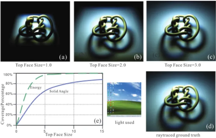
0 5 10 15 0% 20% 40% 60% 80% 100% o C g ar e v r e P ea t n e c e g Energy Solid Angle (c) (d) (b) (c) (e) (b) (a)
Fig. 7. (a), (b), and (c) are renderings using our method with different face sizes. (d) is the ground truth from a ray tracer, using a full representation of the lighting environment at each vertex. (e) shows the coverage ratios of the top face over the upper hemisphere with different sizes. In the graph, the blue solid curve is the top face solid angle covered, and the green dotted curve the energy of a centrally aligned Lambertian lobe. For a standard cube map, its top face size is 2. Top face sizes 3 or 4 can generate visually accurate results.
as a black box that takes this incident lightingLand applies the light transport function T. Therefore, our method can be incorporated into almost any PRT framework and representation forT, including those that are view dependent.
By substituting the angleωiwithvusing appropriate normalizing
weights (numerical cubature), we can write Eq. (28) as
B = L(z,x;v)T(v)dv = i j FiTjDi j(z,x), (31)
whereTj is the wavelet coefficient of the transport functionT(v).
5.2.1 Parameterization. It is common to parameterize the sphere S2 of directions using a cube map consisting of six faces.
Propagations of light to the six faces would require six affine trans-formations. To speed up the computation, we make a trade-off by using only the top face2, but expand its size to cover a larger solid
angle. The top face is aligned with the light plane. Our simplifica-tion is motivated by the observasimplifica-tion that in near-field settings for most vertices, at least one of the lighting, visibility, or BRDF terms would tend to peak at the top face and die out towards peripheral regions. In addition, the cosine term (cosine of the incident angle) reduces contributions towards grazing angles.
We make the top face adjustable so that a large or smaller solid angle can be covered, as needed. The top face in the standard cube map is assumed size 2. Figure 7 shows that midsized faces can cover a sufficient portion of the hemisphere. For example, a size 10 top face covers 82% solid angle of a hemisphere and captures 99% energy of a centrally aligned Lambertian cosine lobe. The surface normal is assumed to be normal to the planar light. Therefore, the top-face approximation works best for the ground plane and other surfaces oriented with their normals similar to that of the light source. Note that the lighting from the planar source will itself peak at the top face and reduce in intensity at other regions. This allows us to extend the approximation to surfaces oriented in other directions as well.
2Similar plane-angle and plane-plane parameterizations have been used in
light field representations [Levoy and Hanrahan 1996; Chai et al. 2000].
In our experiments, sizes 3 or 4 suffice to generate visually accurate results.
5.2.2 Assumptions and Limitations. We have assumed planar area light sources, where the angular distribution of light is uni-form. In Section 7, we discuss extending our relighting algorithm to general 3D lights. We have not implemented, but show theoret-ically (Appendix E) how to handle lights with angular variations such as light fields using ATCs. As noted earlier, we use an ex-panded top-face parameterization that may omit light incident at grazing angles. Our method is general enough to allow interactive scaling, translation, and horizontal rotation of lights and general edits to the light textures. Horizontal rotations are achieved by sim-ply rotating the light textures in the pixel domain, before apsim-plying the wavelet transform. As in most wavelet-based relighting algo-rithms, our algorithm does not support out-of-plane rotations of the lighting. However, in Section 7, we discuss possible approaches to incorporate out-of-plane rotation into our framework.
5.3 Rendering Algorithm
We present key computation steps and major rendering results in this section. All renderings and time measurements are done on a commodity 3.0 GHz Dual-Quad-Core PC with 4GB memory.
5.3.1 Log-Linear-Time Light Propagation. To propagate light, we compute Eq. (30) in 2D,
Lk(z,x)=
i
FiDik(z,x),
wherexandzare 2D variables3, andiandkare, respectively, 2D
vectors of (i1,i2) and (k1,k2). Since we have to loop through all
subscriptsiandk, we only evaluate the equation for nonzero 2D ACCDik(z,x). Variableszand x, respectively, correspond to the
scalesand the translationo. Recall that we useNto denote the total number of basis functions andnfor the number of terms retained after compression. The total cost appears to be the O(nlog2N)
complexity of the 2D ACCs, which is derived in Section 4.4. In fact, a better O(nlogN) algorithm exists if we separate 2D ACCs as products of 1D ACCs and perform the computations in each dimension in succession.
Step 1: ∀i2,k1 Zi2k1(z1,x1)= i1 Fi1i2·Di1k1(z1,x1) Step 2: ∀k1,k2 Lk1k2(z1,z2,x1,x2)= i2 Zi2k1·Di2k2(z2,x2)
Zi2k1is an intermediate variable that carries the accumulation result from the first dimension. Step 1 involves looping over subcriptsi1,
i2 andk1. For any giveni2, over alli1and k1, there are
approxi-matelyO(√nlogN) nonzeroDi1k1(z1,x1) since the complexity of 1D ACCs is about the square root of that of 2D ACCs. Multiplying the number ofi2 which is about
√
n gives the cost for step 1 as
O(nlogN). Similarly, step 2 also takesO(nlogN) time, and thus the total complexity of both steps isO(nlogN). This computation is performed independently for all three color channels.
5.3.2 Precomputation and Rendering. Transport functionsT
are precomputed similarly to Ng et al. [2003], except using the expanded-top-face parameterization. Light propagation (Eq. (30)) involves computing the ACCs. There are two practical approaches,
3Since each vertex has only one depth from the light source, vectorz’s two
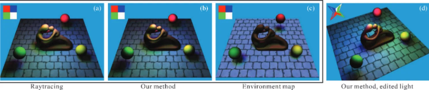
Fig. 8. A diffuse scene of a fertility sculpture and three spheres lit by a simple textured area light. The light textures are shown in the top left corners. The area sources are above the fertility sculpture, but cropped to save space. (a), (b), and (c): Images compare ray tracing, our method, and distant environment map lighting, respectively. Compared to distant lighting in (c), we see that our method in (b) correctly captures the spatially varying shading on the floor and sculpture and generates a result that is quite close to the ground truth. About 1% of source-level and 22% of target-level lighting coefficients are used in our method. (d) Finally, we can edit the light texture and shape, and rotate it in real-time to obtain a distinct appearance in (d). (Note that rotations are limited to horizontal in-plane rotations, and are performed simply in the pixel domain before transforming to wavelets. General out-of-plane rotations are not possible.) This important tool for lighting design would not be possible with previous techniques like precomputed shadow and source radiance fields.
one relying on memory lookups and the other favoring faster computation.
Memory based approach. It is easy to store all nonzero 1D ACCsDik(s,o) compactly in a 4D table and look up their values
dur-ing the computation. Due to the sparsity of ACCs, the cost to com-pute and store the 4D table is minor. As shown in the following table, nonzero ACCs for wavelet order 32 and at spatial resolution 256 only takes 1.06 seconds to precompute and 18.66MB to store. Note that the space and time cost scales close to linearly with the order of the wavelets, confirming our analysis in Section 4.2.4. Precomputed tables at all different orders and resolutions will be downloadable from our Web site (http://www1.cs.columbia.edu/cg/adtpi).
Precomputation and Storage Cost in Memory-Based Approach
space (MB) “Spatial” Resolutions (s, o)
time (S) 64 128 256 512 1024 8 0.26MB 1.05MB0.011S 0.044S 4.22MB0.176S 16.92MB0.708S 67.74MB2.760S 16 0.56MB 2.25MB0.029S 0.114S 9.03MB0.457S 36.24MB 145.09MB1.801S 7.093S 32 1.15MB 4.65MB 18.66MB 74.81MB 299.45MB W av elet Orders (i, j) 0.066S 0.257S 1.059S 4.236S 16.871S 64 2.33MB 9.44MB 37.83MB 151.60MB 606.78MB0.147S 0.589S 2.368S 9.498S 37.768S
Because of the independence of lighting coefficients across vertices, light propagation can be easily parallelized on multicore machines or clusters. We implement both single-thread and multiple-thread rendering algorithms on a 3.0 GHz Dual-Quad-Core machine using the boost library. To ensure workload balance between threads, we choose a round-robin scheduling scheme among a pool of tasks, each carrying a small number (512) of vertices to compute. Compared to the single-thread, an eight-thread implementation generates the exact same rendering result, but improves the speed by about 6.5 times and easily obtains real-time rates. Most of our relighting results are generated using the multithread memory-based implementation.
Computational approach. For machines with faster computa-tion, we tabulateM(r,c) (canonical coupling coefficient defined by Eq. (17)) in a 2D texture and compute ACCs using Eq. (16).M(r,c) is stored using simple angular discretization. SinceM(r,c) is sparse and symmetric (Section 4.2.2), the entire M table can fit into the L2
cache. A 256×256M table in floating point only takes 0.25MB space. In our experiment settings, the computational approach is about half as fast as the memory-based approach.
5.3.3 Nonlinear Lighting Approximation. Realistic illumina-tion can be well approximated using a handful of wavelet coeffi-cients. Our model allows compression at two levels, of both the original light F (source level) and the local incident radianceL
(target level), drastically speeding up the performance.
Source-level compression. At the source level, lighting coef-ficientsFiare ordered, and the most significant ones are picked, as
in standard PRT. Using only 1% of source-level coefficients usually generates accurate renderings for our test scenes, as shown in Fig-ures 8 and 9. In general, the compression depends on the BRDF of the receiver as well as the distance between emitter and receiver.
Target-level compression. Target lighting coefficientsLkvary
across all vertices and change as the light source is dynamically updated. It is difficult to predetermine which target coefficients are important, and generating and sorting them in real time is too expen-sive. Instead, we assume a heuristic light ˜Fiand precompute lighting
predictions ˜Lkfor a number ofzandxvalues. The light predictions
˜
Lkare used to pick target lighting coefficientsLkat runtime. ˜Lk(z,x)=
i
˜
FiDik(z,x). (32)
Rarely will the lighting predictions ˜Lk be exactly the same as the
actual lightingLk. They will, however, roughly track how power
distributions of the wavelet coefficients under affine transformations change with respect to spatial locations. We use a simple constant light heuristic (a vector with only DC, [1,0,0, . . .]) in our experi-ments, and need about 20∼30% of target-level lighting coefficients for visually accurate results, as shown in Figures 8 and 9. 5.4 Results
We demonstrate three scenes: fertility (39,391 vertices, Figure 8), chairs (59,995 vertices, Figures 1(b) and 9(a)–(c)), and couches (68,046 vertices, Figures 1(a) and 9(d)–(f)). All scenes have static geometries and are rendered using PRT, with near-field lighting effects generated using our method. The chairs, tables, and couches have specular materials with precomputation done per vertex [Ng et al. 2003]. The fertility scene is diffuse and can be viewed from
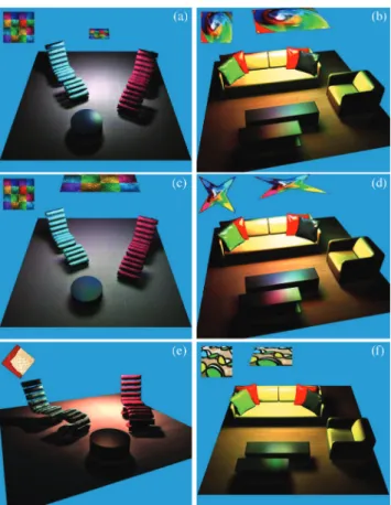
Fig. 9. Two specular scenes rendered with near-field sources using our method. Light textures used are shown in the upper left corners, and their sizes and positions vary. In the chair scene, note the sharper and larger shadows underneath the chairs when the light is small and close (a), and smaller and softer shadows when the light is larger and far away (b). Also note in the couch scene how light editing (change texture, reshape) from (d) to (e) influences specular reflections on the tables and cushions. Figure 1(a) follows (e) but resizes and rotates the light. (c) and (f) render both specular scenes from another view point with a different light texture. Specular rendering from a different viewpoint requires a separate precomputation. Close-ups can be found in Figure 1. Performance numbers are reported in Figure 11.
different angles. Please note that our technique is orthogonal to many PRT calculations and can certainly be used with view-dependent methods such as BRDF in-out factorization [Wang et al. 2004; Liu et al. 2004] or other approaches. In all cases, we can interactively edit the light.
5.4.1 Near-Field vs. Distant Lighting Effects. In Figure 8(b), we light a diffuse fertility scene with near-field lights. Spatially varying shadings and colored soft shadows on the floor are clearly visible. In contrast, Figure 8(c) shows a rendering using the standard environment mapping technique,4which fails to capture the shading
variations on the floor or sculpture that are critical to the mood of the scene.
In Figure 9, we render two specular scenes with a number of lights at different positions. In particular, when the light is closer to the floor in Figure 9(a) (as compared to Figure 9(b)), shadows of both
4The incident lighting at the center of scene is used as the “environment
map” and fed to all vertices for shading computations.
Fig. 10. Approximation errors of the source-(graph (a)) and target-(graph (b)) level compressions. Four representative light textures with different levels of high frequencies are used. The horizontal axes are on a log scale.
chairs expand sideways and the specularity on the table focuses. In Figures 9(d)–(e), we can clearly observe how editing the light texture, as well as its shape and size, changes the specular highlights on the tables and cushions. These effects are hard to capture with distant illumination. Close-ups are found in Figures 1(a) and 1(b).
5.4.2 Light Editing. We develop a prototype light editing and design system, which allows artists to edit the lights in a more intu-itive and interactive way. An artist can move, resize, or horizontally rotate the light. Note that these operations on the light source are all performed once per frame in the pixel domain, before transforming the lighting into wavelets and propagating to the vertices. Lights can also be textured. Image processing methods such as blending, filtering, warping, and painting can be easily applied to edit the light texture. Because the cost of compressing the edited light texture into wavelets in real time is minor, changes can be immediately reflected in the realistically rendered images using our algorithm. For exam-ple, starting from Figure 9(d), we first paint and reshape the light to obtain Figure 9(e), and then resize and rotate the light to generate the image in Figure 1(a). Note the generality of our system to han-dle textured and editable/reshapeable light sources in Figures 8 and 9, which cannot be addressed by previous near-field lighting tech-niques like precomputed source radiance fields [Zhou et al. 2005].
5.4.3 Accuracy Analysis and Validation. We compare the ground-truth image from a ray tracer in Figure 8(a) with our re-sult in Figure 8(b). We also showed a ground truth comparison in our didactic example of a knot scene in Figure 7. Since we only use a finite plane to parameterize the upper hemisphere, light incident at grazing angles is omitted, resulting in dimmer shading for some boundary vertices and the lack of grazing angle specularities. Also, lighting coefficients are compressed at both the source and target levels. Thus, energies at certain frequencies may be lost. Neverthe-less, Figures 7 and 8 clearly demonstrate that our results show little visual difference from the ground truth, but now can be rendered at real-time rates. Similar results hold for our other images.
Lighting approximation error. Figure 10 shows the approxi-mation errors for different compressions at both source and target levels. A few representative light textures used in the renderings are included in the accuracy analysis. Note that the horizontal axes in Figure 10 are on a log scale. The approximation accuracy improves quickly with increasing numbers of coefficients used. In addition, the target-level compression is less efficient than the source-level, requiring more coefficients for the same level of accuracy. This
Source=1% Target=20% 38.71fps 7.58fps 25.87fps 4.52fps 23.34fps 3.91fps Source=1% Target=1% 151.86fps 32.79fps 107.33fps 20.43fps 101.64fps 18.60fps Source=5% Target=40% 24.83fps 4.17fps 12.48fps 2.03fps 11.98fps 1.94fps Source=100% Target=100% 7.04fps 1.08fps 4.86fps 0.75fps 4.80fps 0.71fps Source=20% Target=70% 13.78fps 2.17fps 7.87fps 1.15fps 7.31fps 1.10fps #Verts 39,391 56,995 68,046 Scenes fertility chairs diffuse specular specular couches Threads
Fig. 11. Rendering performance with different compressions. For each scene, the upper row contains the performance numbers using the multi-thread implementation, and the lower row for the single-multi-thread implemen-tation. All performance is measured on a 3.0 GHz Dual-Quad-Core PC with 4.0 GB memory. The second and third performance columns correspond to realistic compression levels for accurate rendering, and achieve real-time rates for both the single-thread and multithread algorithms.
inefficiency is due to the fact that we rely on a constant heuristic light to predict significant lighting coefficients after the affine trans-formation. Our experiments show that 1% of the source-level and 20∼30% of the target-level lighting coefficients (using a constant light heuristic) usually suffice to generate visually accurate results. 5.4.4 Performance. All images are rendered at 1200×900 res-olution and a wavelet order of 32. The rendering speed depends on a number of factors such as the total number of vertices, numbers of the retained source- and target-level lighting coefficients, and the complexities of the scene materials. In Figure 11, we report the rendering performance for the fertility, chair, and couch scenes. As shown in the second and third performance columns (which corre-spond to the common compression usage), our algorithm provides real-time performance, as also seen in the supplemental video that can be accessed through the ACM Digital Library.
5.5 Discussion and Comparison to Previous Near-Field Relighting Methods
In comparison with previous techniques, our method offers signifi-cant design flexibilities and achieves effects that are otherwise hard to capture. Annen et al. [2004] and Wang et al. [2006a] pioneered rendering midrange illuminations, using, respectively, spherical har-monic gradients and scaling. Lights are assumed some distance away from the scene so that the lighting can be smoothly interpolated and its propagation (affine transformation) approximated. Our work can be seen as extending these methods to near-field settings, as shown in Figure 8. Moreover, our technique can also render specular scenes, such as the chair and couch scenes in Figure 9. Zhou et al. [2005] and Kristensen et al. [2005] made important advances in near-field rendering of both diffuse and specular scenes. The light content, however, is built into the precomputations and has to remain static during rendering. Designers can move the light or change its inten-sity, but cannot edit the light shape or texture. Our method can be seen as an important generalization of their techniques, and allows light editing to be fully integrated with any PRT framework. For ex-ample, interactively painting the lights and changing their shapes, as done in Figures 8(d) and 9, or quickly flipping through several arbi-trary light textures during relighting, as demonstrated in the video, are all feasible with our method. Finally, Annen et al. [2004], Wang et al. [2006a], and Kristensen et al. [2005] base their methods on the spherical harmonic basis and cannot capture all-frequency effects. 6. OTHER APPLICATIONS
Besides our main problem of PRT near-field relighting, affinely transformed wavelets and wavelet integrals have many other poten-tial applications in rendering, image and signal processing, and
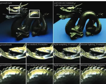
nu-Fig. 12. A gold dragon under a near-field area source rendered using wavelet importance sampling. The ground-truth rendering is at the top left. To compare near-field and distant lighting effects, we also show an image rendered using uniform environment lighting at the top right. The color of the environment lighting is the average of the textured area light used in the near field. Shading variations and shadows are clearly different under the two lighting conditions. Under near-field lighting, the dragon exhibits high color contrast and strong directional specular reflections, while the shading under environment lighting is significantly diffused out. In the close-ups, for the same number of samples (8), we compare the result of our method with those by standard wavelet importance sampling but assuming that the light is distant (distant lighting is used to generate important samples, but shading is calculated using the area light), and light importance sampling (light sampling). Order 64 wavelets are used for all three sampling meth-ods. Our method converges to the ground truth an order of magnitude faster, exhibiting substantially less noise at this sample count.
merical analysis. As a first proof of concept, we demonstrate initial examples of wavelet importance sampling with near-field lighting for offline Monte Carlo rendering, and image dilation and translation directly in the wavelet domain for image processing.
6.1 Wavelet Importance Sampling
Clarberg et al. [2005] have shown that importance sampling the product of the BRDF and the distant lighting can greatly reduce the variance in Monte Carlo rendering. However, their method is limited to distant environment map lighting, since lighting-BRDF products are computed using standard triple product integrals. Our theory enables a direct extension to the near-field setting, with planar area sources. We pretabulate BRDFs as 4D functions as done in Clarberg et al. [2005]. For each pixel, we affinely transform the original light source into the local incident radiance using Eq. (30) of Section 5, in a very similar fashion as for relighting. We then multiply the wavelet coefficients of the local radiance with those of the BRDF using the standard triple product wavelet integral [Ng et al. 2004]. Thereafter, we perform hierarchical wavelet warping to obtain importance samples, used for Monte Carlo estimation. Distinct from Clarberg et al. [2005], we use the standard wavelet decomposition and an expanded-top-face parameterization, as we do in Section 5 for relighting.
We demonstrate a near-field rendering of a gold dragon under an area light source in Figure 12. We observe visual effects such as highly contrasted and spatially varying shadings that are hard