Efficient BMC for Multi-Clock Systems with Clocked Specifications
Malay K Ganai and Aarti Gupta
NEC Laboratories America, Princeton, NJ USA 08540
Abstract - Current industry trends in system design — multiple clocks, clocks with arbitrary frequency ratios, multi-phased clocks, gated clocks, and level-sensitive latches, combined with clocked — pose additional challenges to verification efforts. We propose an integrated solution that improves SAT-based Bounded Model Checking (BMC) by orders of magnitude, for verification of synchronous multi-clock systems with clocked LTL properties. Our main contributions are: a) Efficient clock modeling schemes to handle clock related challenges uniformly, b) Generation of automatic schedules and clock constraints to avoid unnecessary unrolling and loop-checks in BMC, c) Dynamic simplification of BMC problem instances with clock constraints, and d) Customized BMC translations—with incremental formulations and learning—to directly handle PSL-style clocked specifications. We demonstrate the effectiveness of our approach on some OpenCores multi-clock system benchmarks.
I Introduction
A continuing push for high performance and low power designs has greatly increased the system design complexity. One norm of today’s System-on-Chip (SoC) design is the use of multiple clocks and phases, and gated clocks. This paradigm shift from a single global clock synchronous design paradigm was inevitable, as distributing a single clock across the increasing size of die, number of latches, frequencies of clocks and delays of wires poses a major bottleneck in achieving the goals of higher performance and lower power [1]. For power-conscious designs, designers often use gated clocks to reduce or disable the switching activity of certain portions of the design. Furthermore, SoC designs comprise several intellectual property (IP) blocks that operate at different clock frequencies and need to communicate across asynchronous clock domains. Each of these design styles increases the verification complexity in terms of increased number of state bits and deeper bug traces.
Formal verification techniques like SAT-based Bounded Model Checking (BMC) [2-5] due to several advancements — improved DPLL-style SAT solvers [6], on-the-fly circuit simplification [7, 8], partitioning and incremental BMC formulation [9], and SAT-based incremental learning [8, 10, 11] — have been gaining wide acceptance as a scalable solution compared to BDD-based symbolic model checking [12]. The performance of SAT-based BMC is less sensitive to the number of flip-flops (FFs) and does not suffer from space explosion.
A.
Motivation
An integrated solution to verify multi-clock systems comprising multiple clocks, clocks with arbitrary frequency ratios, multi-phased clocks, gated clocks, level-sensitive latches, combined with clocked specification, that exploits recent advancements in SAT-based BMC has been lacking. Previously proposed solutions have been largely piece-wise, such as translating clocked LTL properties [13] that can be handled by a standard BMC solver, reducing the verification model size by using phase abstraction techniques [14-17], and generating a clocking
scheme from given frequency constraints based on event queue semantics to avoid unnecessary unrolling during BMC [18].
The following design features and specifications of clocked systems pose additional challenges that can limit the application and effectiveness of these previous approaches:
1. Specifying sub-formulas on various clocks: Property variables that involve gates with support from state elements in multiple clock domains require the use of clocks in the formula to avoid ambiguities. The Property Specification Language (PSL) standardized by Accellera [19] has formal semantics for specifying clocked properties using the clock operator @, based largely on the work of Eisner et al. [13]. The general translation scheme for clocked properties tends to generate large nested LTL formulas that can limit the effectiveness of a standard BMC solver. For example, a clocked LTL formula F(p∧ (Xq@clk1)@clk) gets translated into an unclocked LTL formula F(p∧(!clkU(clk∧X(!clkU(clk∧(!clk1U(clk1∧ q))))))).
2. Multiple clocks with arbitrary frequencies, ratios and multiple phases: Generating a verification model naively that ticks on a global clock with a frequency derived from the least common multiple (LCM) of various input clock frequencies is quite inefficient (multiple phases effectively multiply the clock frequencies). In particular, the BMC problem instances with no corresponding clock events become an unnecessary computational overhead.
3. Gated Clocks: Gated clocks limit the static simplification [17] of a verification model due to its non-periodic behavior.
4. Latches (level-sensitive) used with flip-flops (edge-triggered): For verification purpose [16], latches are modeled as flip-flops clocked on a global clock in synchronous designs. Clocked specifications with latch enabling clocks pose further verification challenges.
B. Related Work
Here we discuss the limitations of various approaches that have addressed some of the above-mentioned challenges. In approaches [15-17], the goal is to reduce the number of state elements in the model using phase abstraction techniques. First, clock-like signals, which exhibit periodicity, are identified manually or by using 3-valued simulation [17]. Based on these clock signals, they identify non-overlapping latch layers (or phases), and then retain latches in one layer as flip-flops, and replace latches in the remaining layer by wires or multiplexers. Subsequently, they obtain a verification model by making C (=#phases) copies of the transition relation and simplifying the logic by propagating the phase values of clock signals. However, the presence of gated clocks and multiple clocks with arbitrary clock frequencies and ratios can severely restrict the identification of clock-like signals (and various phases) and therefore, limit the size reduction of the verification model. Note that these approaches focus mainly on reducing the number of flip-flops in order to improve the scalability of BDD-based model checking, and not so much on reducing the number of logic gates.
In another approach by Clarke et al. [18], given multiple clock frequency constraints, a clock state machine is built based on event queue semantics. Each clock state maps to a configuration (i.e., a
set of events) in an event queue where each event corresponds to a tick of an active clock. They formulate a BMC problem instance by unrolling the design composed with the clock state machine only at clock events, thereby avoiding the redundant unrollings. However, the authors have not proposed any solution to combine their approach with dynamic simplification procedures in the BMC framework, or to handle clocked specifications.
Ganai et al. [9] have proposed techniques for customized translation of commonly occurring (un-clocked) properties in BMC by using partitioning and incremental formulation, to improve the scope of SAT-based incremental learning. The approach was shown to be more efficient in practice than the standard monolithic BMC formulations [2, 4]. However, as clocked property translation [13] often leads to large and deeply nested formulas, it is difficult to customize each such translation.
C. Our Contributions: Overview
In practice, it is important to address the scalability issues in verifying multi-clock systems with clocked specifications. Understanding the significance of BMC customization and the difficulties in handling translated clocked properties in a multi-clock system, we propose an integrated BMC-based solution as follows:
1. We propose a uniform clock modeling scheme to handle multiple clocks with arbitrary frequencies and ratios, gated clocks, multiple phases, latches and flip-flops in multi-clock synchronous system, to obtain a single-clock model.
2. Given clock characteristics, we automatically generate schedules and clocks constraints based on event queue semantics to eliminate redundant unrollings and loop-checks. 3. Since not all clock domains are active at each unrolling, we
perform dynamic simplification of the unrolled transition relation using the clock constraints at each unrolling, where we re-use the current unrolled sub-circuit corresponding to an inactive clock-domain for the next unrolling; thereby reducing size of the BMC problem instance.
4. We also propose novel BMC customization for translation of clocked properties directly rather than customizing each translated unclocked property, and simultaneously offer the benefits of partitioning and incremental BMC formulation [9]. Though we discuss such customization for the clocked LTL (F(f))@ it can be extended to other clocked LTL such as (F(f∧G(g)))@ where f, g are clocked expressions with atoms propositionally combined with nested X operators. Note, our customized translations are more efficient than the previously proposed general translations for clocked properties.
Outline: We give background on clocked LTL specifications and BMC customization for un-clocked properties in Section II; we discuss our contributions in Sections III-V with description of modeling, and generation of schedules and constraints in Section III, dynamic simplification in Section IV, and BMC customization for clocked properties in V; we discuss our experimentation on OpenCores [20] benchmarks in VI; and conclusions in VII.
II. Background
A. Clocked LTL Specifications
A clocked LTL specification (f)@clk, expressed under the context of clk (that is always ticking) using the clock operator @, can be equivalently translated [13] into an un-clocked LTL specification (with an implicit global clock tick) Tclk(f)(≡ (f)@clk) where Tclk(f) is defined recursively using the following rules R1-6:
R1: Tclk(p) = ¬clk U (clk ∧ p) // f is propositional atom p R2: Tclk(¬f) = ¬Tclk(f) R3: Tclk(f1∧ f2) = Tclk(f1)∧ Tclk(f2) R4: Tclk(X f) = ¬clk U (clk∧X(¬clk U (clk∧ Tclk(f))) R5: Tclk( f1U f2) =(clk → Tclk(f1))U (clk ∧ Tclk(f2)) R6: Tclk((f)@clk1) = Tclk1(f)
Rules for other LTL operators F,G and Wcan be derived from the above rules. Note, that in [13], the authors have differentiated temporal operators and propositional atoms as weak or strong using the strength operator !. For ease of understanding our approach, we will assume that clocks in the specifications are always ticking and therefore, the strength operator ! can be dropped.
We first make some crucial observations regarding the rules R1, R4 and R6. As per rule R1, p@clk holds at the current state, if either p holds and clk ticks at the current state, or clk ticks next at a state where p also holds. Similarly, as per rule R4, (Xf)@clk takes us two clk ticks into the future if clk does not hold in the current state. The rule R6 disallows accumulation of clocks in the presence of nesting, allowing only the innermost specified clock to supersede the outer ones.
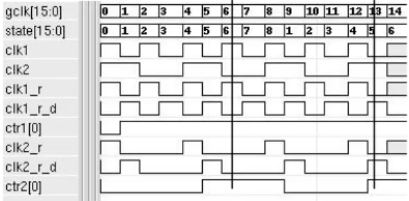
Example: Consider two clocked LTL formulas, P1 and P2. P1: F(ctr2[0] * (X(ctr2[0]))@clk2_r_d) P2: F((ctr2[0] * X(ctr2[0]))@clk2_r_d)
In P1, ctr2[0] (bit 0 of ctr2) is clocked by the global clock, gclk, while in P2 it is clocked by clk2_r_d as shown in Figure 1. One can verify that the witness state for P1 is at gclk=6 where ctr2[0]=1 and also two clk2_r_d ticks later ctr2[0]=1 at gclk=13. On the other hand, P2 does not have a witness on the path shown. These subtleties in the clocked specifications add further complexity to the BMC method based on customized translation, described next.
Fig. 1: Example timing diagram for clocked specification
B.
BMC Customization of Unclocked LTL Specifications
Instead of the standard monolithic translation in BMC, as originally proposed by Biere et al. [2], Ganai et al. [9] use customized property translations to build and solve a BMC problem incrementally, by partitioning it further into several simpler SAT sub-problems. Further, the incremental formulation has been effectively combined with several SAT-based learning techniques, such as those from shared constraints (L1) [10, 11], previous satisfiable (L2) [10] and unsatisfiable (L3) results [8]. This enables learning between sub-problems not only across time frames, but also within the time frames.
We briefly describe the customized translation (refer [9] for details) and various learning aspects for a negated (unclocked) safety property, i.e., F(f) in the procedure BMC_solve_F as shown in Figure 2. For simplicity, we consider f to be a propositional atom. (Later, we discuss how f can be extended to allow nested X
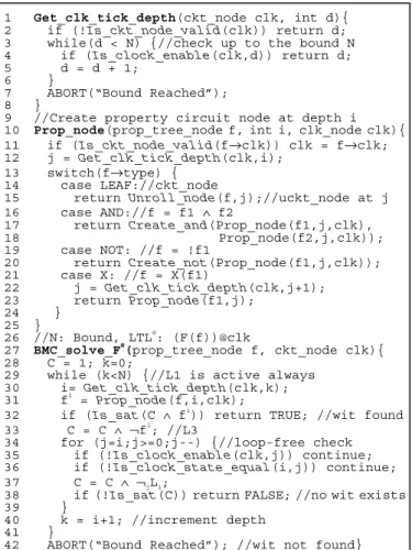
operators with propositional logic in the context of clocks.) The sub-procedure Is_sat(C) denotes a SAT check of the Boolean formula C;L1-L3 denote various incremental SAT-based learning techniques as mentioned above; jLi denotes the loop transition constraint, i.e., jLi = T(si, sj), transition from state si to sj; N denotes the user-provided bound. The Boolean constraint fi (line 4), denotes the property node f at the ith unrolling, obtained using Unroll_node procedure. One can use circuit simplification with a compose operator such as [8], to obtain the unrolled circuit nodes. The satisfiability of sub-problem (C∧ f i) is checked at depth i (line 5). If it is satisfiable, the procedure returns true indicating the witness found; otherwise, ¬fi is learned (L3) and added to C (line 6). If the current path cannot be extended to remain loop-free (lines 7-10), the procedure returns false, indicating that no witness is possible. When (i≥N ), the procedure aborts (line 13).
1 BMC_solve_F(prop_tree_node f){ 2 C = 1; i=0;
3 while (i<N) { //L1 is active always 4 fi = Unoll_node(f,i);
5 if (Is_sat(C ∧ fi)) return true; //wit found 6 C = C ∧ ¬fi; //L3
7 for (j=i;j>=0;j--) {//loop-free check 8 C = C ∧ ¬jLi;
9 if (!Is_sat(C)) return false; //no wit exists 10 }
11 i = i+1; 12 }
13 ABORT(“Bound Reached”); //wit not found }
Fig. 2: BMC Customization for un-clocked
F
(f)
III. Modeling Multi-Clock Systems
A. Uniform Clock Modeling Scheme
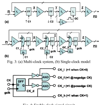
We consider modeling of synchronous multi-clock systems that have clocks with arbitrary but known fixed frequencies, and fixed initial phases. Multi-clock systems with the clocks derived from a single source generator lead to synchronized clocks with fixed frequencies and known initial phases. However, if the clocks are generated from independent sources, they are in general unsynchronized, typically with fixed frequencies but unknown initial phases. For modeling such systems, we consider one representative at a time from the various combination scenarios of initial phases, unlike the work of Clarke et al. [18] where all possible scenarios are considered simultaneously in modeling. Our goal is to trade generality for scalability of the BMC methods. Consider a synchronous multi-clock example shown in Figure 3(a). Here, Xis a set of FFs triggered on positive edge (↑) of input clock C1; Yis a set of FFs triggered on negative edge (↓) of input clock C2; Zis a set of level-sensitive latches triggered on active high of gated clock GC; f1-f5 are combinational blocks; PI the set of primary inputs; and PO the set of primary outputs. Note, “/” on the connectors (→) indicates multiple connecting wires.
We derive a single-clock model, as shown in Figure 3(b), such that value change on inputs, internal signals and state elements occurs only at the tick of gclk. In order to do so, we add multiplexers in the next state transition logic of X, Y, and Z; and generator circuits g1-g3 (details shown in Figure 4) for enable clocking signals C1_r, C2_f, and GC_h that take value 1 at the posedge of C1,negedge of C2, and high value of GC, respectively. For example, the clocking signal posedge C1 is modeled using the enable clocking signal C1_r=C1∧¬C1_d, where C1_d represents clock C1 delayed by one gclk.
Fig. 3: (a) Multi-clock system, (b) Single-clock model
Fig. 4: Enable clock signal circuit
B. Generation of clock schedules and constraints
For fixed input clock frequencies and initial phases, one can model aclock-generator ticking on gclk with frequency equal to LCM of the frequencies of all input clocks, and use the clock-generator to compute deterministically the values of input clocks at each tick of gclk. For SAT-based BMC, unrolling a single-clock model at every tick of gclk would add computational overhead, as there may be some ticks when no input clocks change values (and so the state elements). Instead, we use event queue semantics [18], where only those ticks of gclk are considered when at least one input clock changes value. We now discuss the derivation of relevant ticks, i.e., clock schedules, and clocking constraints on the input clocks, using an example as shown in Figure 5.
Fig. 5: Ticks of global clock gclk
Let frequencies of input clocks C1 and C2 be 100Mhz (time period, TC1=10ns), and 62.5Mhz (TC2=16ns), respectively, and let the initial phases be 0ns and 4ns, respectively. Edge direction in the Figure 5 indicates the active edge. Under the event queue semantics, events are recorded chronologically where each event corresponds to a value change of input clocks C1 and C2. Let a 3-tuple Si=<ti,c1i,c2i> denote a configuration corresponding to the ith recorded event in the queue at time ti, with c1i and c2i representing the values of clock signals C1 and C2, respectively. In the event queue, we obtain the following configurations for 0≤t≤30: S0=<t0=0,1,1>,S1=<t1=4,1,0>,S2=<t2=5,0,0>,S3=<t3=10,1,0> S4=<t4=12,1,1>,S5=<t5=15,0,1>,S6=<t6=20,1,0>,
S7=<t7=25,0,0>,S8=<t8=28,0,1>,S9=<t9=30,1,1>.
Observe that state elements cannot get updated between the C1 C2 GC gclk 0 4 5 1012 15 20 25 2830 35 freq=62.5M ns freq=100M C1 C2 GC gclk 0 4 5 1012 15 20 25 2830 35 freq=62.5M ns freq=100M FF f2 f1 f3 ↑C1 ↓C2 PI X PO FF L f5 f4 Y Z GC FF f2 f1 f3 C1_r C2_f PI X PO FF FF f5 f4 Y Z GC_h gclk 0 1 0 1 gclk 0 1 gclk g1 g2 g3 C1 C2 (a) (b) FF f2 f1 f3 ↑C1 ↓C2 PI X PO FF L f5 f4 Y Z GC FF f2 f1 f3 C1_r C2_f PI X PO FF FF f5 f4 Y Z GC_h gclk 0 1 0 1 gclk 0 1 gclk g1 g2 g3 C1 C2 (a) (b) CK_r (=1 @posedge CK) CK_f (=1 @ negedge CK) DFF D Q AND CK_h (=1 when CK=1) CK_l (=1 when CK=0) CK gclk CK_d AND CK_r (=1 @posedge CK) CK_f (=1 @ negedge CK) DFF D Q AND CK_h (=1 when CK=1) gclk CK_d AND CK_r (=1 @posedge CK) CK_f (=1 @ negedge CK) DFF D Q AND CK_h (=1 when CK=1) CK_l (=1 when CK=0) CK gclk CK_d AND CK_r (=1 @posedge CK) CK_f (=1 @ negedge CK) DFF D Q AND CK_h (=1 when CK=1) gclk CK_d AND
consecutive configurations, i.e., Si and Si+1. Thus, we generate clock schedules for BMC unrolling by considering only those ticks of gclk that correspond to these configurations, with Si occurring at ith tick. We also generate clocking constraints at the ith tick or ith unrolling by constraining input clock signals such as C1 and C2 with the tuple values c1i, and c2i. During witness generation, we use ti to time-stamp the ith depth in the witness trace.
C. Repetition Period and Recurrence Length
Using the same example above, we now discuss the repetition of configurations and its significance in removing some loop-checks jLiin BMC between unrollings at the i
th
and jth tick of gclk. Two configurationsSi=<ti,c1i,…,cni> and Sj=<tj,c1j,…,cnj> are said to be equivalent (i.e., recur every R ticks of gclk), if and only if ∀0≤k<R (∀0≤m<n (cmi+k=cmj+k)) and ∃o(∀0≤k<R (ti+k-tj+k=o)). In other words, the corresponding successive configurations have matching clock signal values and have a fixed time difference. We call R the recurrence length. The repetition period T of the clock-generator (i.e., when clock states repeat) can be obtained by taking the LCM of the clock periods TC. Note, the equivalent configurations correspond to equivalent clock states. For our running example, the repetition period T=80ns (LCM of 10ns and 16ns) and recurrence length R=26. We use this information in BMC to consider loops-checks jLibetween unrolling depths i and j only if (i-j) mod
R=0, i.e., when the clock states at the ith and jth ticks are the same. (Note, the clock states are not equivalent otherwise.)
To summarize so far, we first generate a single-clock model from the given multi-clock system. From the input clocking characteristics, we derive clocking constraints, automatic schedules, and the recurrence length, and use them in BMC as described later.
IV. Dynamic Simplification in BMC
The presence of gated clocks and clocks with arbitrary frequencies limits the effectiveness of phase abstraction techniques in static simplification of the verification model [17]. We overcome this limitation by applying dynamic simplification during unrolling, where simplification need not depend explicitly on the periodicity of clocking signals. We discuss the dynamic simplification of the unrolled model to reduce size of the BMC problem instances using clock constraints generated as above, using the multi-clock example and corresponding single-clock model as shown in Figures 3(a) and 3(b), respectively, introduced in Section III.A. We use the clocking characteristics of inputs clocks C1 and C2, and assume the dynamic behavior of gated clock GCas shown in Figure 5, with the initial states C1_d=0 in the circuit g1 and C2_d=1 in the circuit g2. Note, the dotted arrows indicate cause-effect relations, as GC is a (combinational) function of Y FFs, clocked by C2. The transfer functions for the single-clock model are as follows:
NEXT(X) = (C1_r) ? f1(Z,PI) : X; // s?b:c ≡ ITE(s,b,c) NEXT(Y) = (C2_f) ? f2(X) : Y;
NEXT(Z) = (GC_r) ? f3(Y) : Z; PO = f5(Z);
We use the scheduling of gclk as shown in Figure 5 to unroll the model in BMC. We constrain the input clocks C1 and C2 at the ith unrolling using the clocking constraints at the ith tick. In the following, we use an 8-tuple UCi= <PIi;C1_ri;C2_f i;GC_hi; Xi;Yi;Zi;POi> to denote the ith (i≤8) unrolled circuit nodes (combinational logic) for PI, C1_r, C2_f, GC_h, X,Y, Z, and PO, respectively, with X0,Y,0 and Z0 denoting respective initial states. UC0= <PI0;1;0;0;X0;Y0;Z0;PO0=f5(Z0)>
UC1 = <PI1;0,1,0;X1=f1(Z0,PI0);Y1=Y0;Z1=Z0;PO1=PO0> UC2 = <PI2;0;0;1;X2=X1;Y2=f2(X1);Z2=Z1; PO2=PO1>
UC3 = <PI3;1;0;1;X3=X2;Y3=Y2;Z3=f3(Y2); PO3=f5(Z3)> UC4= <PI4;0;0;1;X4=f1(Z3,PI3);Y4=Y3;Z4=Z3;PO4=PO5> UC5= <PI5;0;0;1;X5=X4;Y5=Y4;Z5=Z4;PO5=PO4> UC6= <PI6;1;1;1;X6=X5;Y6=Y5;Z6=Z5;PO6=PO5>
UC7=<PI7;0;0;0;X7=f1(Z6,PI6);Y7=f2(X6);Z7=Z6;PO7=PO6> UC8= <PI8;0;0;0;X8=X7;Y8=Y7;Z8=Z7;PO8=PO7>
Note that by using dynamic simplification, UC8has far fewer copies of combinational blocks in its cone-of-influence (COI) than without its use, i.e., three f1, two f2, one f3 and two f5, compared to nine copies each of f1,f2,f3, and f5. This is due to our simplification where the circuit nodes of a clock-domain in one time frame map to those of the previous time frame, if the clocking signal for that domain is inactive in the previous time frame. For example, circuit nodes X3and X2 map to X1as C1_r=0 at i=1,2. We also use on-the-fly circuit simplification procedures [7, 8] for further compacting the unrolled circuits.
V. Customization of Clocked Specifications in BMC
Given a clocked specification of the form (F(f))@clk, we present our BMC customization using the procedure BMC_solve_F@ as shown in Figure 6. We allow fto be a Boolean combination of
nested X operators with propositional atoms, where
sub-expressions can have clocks specified with @. For our discussion in this paper, we only allow input clocks in the design to be in the support (i.e., COI) of clk in the specification. For example, a clocked specification can be of the form (F(p ∧ ¬X(q ∧ X(r))@clk1))@clk with input clocks only in COI of clk and clk1. Note that the specification clock clk corresponds to the enable clock signal in our single-clock model.
We construct a tree expression for f where each node prop_tree_node represents a sub-expression. Each node is of type AND (∧), NOT(¬), LEAF, or X, where LEAF corresponds to a propositional atom. Note, we use ckt_node to denote a propositional atom or gate in the transition relation, and uckt_node such as fito denote a propositional logic node corresponding to the ith unrolling of f. For a prop_tree_node g, we use g→clk to denote the associated specification clock.
We first discuss the procedures used in BMC_solve_F@. The procedure Is_clock_enable(clk,d) (lines 4, 35) returns true if clk evaluates to 1 at depth d, and returns false otherwise. Note, as we allow only input clocks in COI of clk, we obtain the value of clk by simulating the logic circuit in its COI until d, using the values on the input clock constraints. The procedure Get_clk_tick_depth(clk, d) (lines 1-8), uses Is_clock_enable to determine when clk ticks next, starting from depth d. The procedure Is_ckt_node_valid returns false if clk is not valid, i.e., for unclocked property. (Note, for invalid clk, procedure Get_clk_tick_depth returns d.)
Now, we discuss the procedure BMC_solve_F@ for an
unclocked LTL formula F(f), and compare it with BMC_solve_F (Figure 2) in the presence of nested X’s in f. In the absence of associated clk, the procedure Get_clk_tick_depth (lines 12, 22, 30) returns value equal to its input (e.g., j=i at line 12) as Is_ckt_node_valid(clk) returns false at line 2. The procedure Prop_node (line 31) returns fi using the procedures Unroll_node (line 15), Create_and (line 17), and Create_not (line 20). If f→type is X,the current unroll depth is advanced by one (line 22). The rest of the description of BMC_solve_F@ is similar to BMC_solve_F, except lines 35-36 which are relevant only for a valid clock. For clocked properties, we do additional pruning of loop checks using the procedure Is_clock_state_equal(i,j) (line 36) which returns true if and only if ((i-j) mod R) = 0 where R is the recurrence length (Section III.C). The correctness of the translation for unclocked LTL is based on the re-write rules: ¬Xf≡X¬f, and X(f∧X(g)) ≡X
f∧ XXg. Note, we choose to build a uckt_node f i, instead of partitioning the problem into separate conjunctions/disjunctions of X operators and propositional atoms. In our experience, too many SAT sub-problems add a performance overhead and thus, we restrict our sub-problem partitioning at conjunctions/disjunctions with one operand being F or G. Also, the procedure Prop_node allows sharing of common sub-expressions in f by mapping identical structures of uckt_node logic nodes, using on-the-fly simplification procedures during unroll [7, 8].
Example: For the given LTL F(p∧¬X(q∧X(r))), the procedure Prop_node(f,i,NULL) at depth i (NULL denoting no associated clock) returns the Boolean expression f i= pi∧¬ (qi+1 ∧ ri+2). 1 Get_clk_tick_depth(ckt_node clk, int d){ 2 if (!Is_ckt_node_valid(clk)) return d; 3 while(d < N) {//check up to the bound N 4 if (Is_clock_enable(clk,d)) return d; 5 d = d + 1;
6 }
7 ABORT(“Bound Reached”);
8 }
9 //Create property circuit node at depth i 10 Prop_node(prop_tree_node f, int i, clk_node clk){ 11 if (Is_ckt_node_valid(f→clk)) clk = f→clk; 12 j = Get_clk_tick_depth(clk,i);
13 switch(f→type) { 14 case LEAF://ckt_node
15 return Unroll_node(f,j);//uckt_node at j 16 case AND://f = f1 ∧ f2
17 return Create_and(Prop_node(f1,j,clk), 18 Prop_node(f2,j,clk)); 19 case NOT: //f = !f1
20 return Create_not(Prop_node(f1,j,clk)); 21 case X: //f = X(f1) 22 j = Get_clk_tick_depth(clk,j+1); 23 return Prop_node(f1,j); 24 } 25 } 26 //N: Bound, LTL@: (F(f))@clk 27 BMC_solve_F@ (prop_tree_node f, ckt_node clk){ 28 C = 1; k=0;
29 while (k<N) {//L1 is active always 30 i= Get_clk_tick_depth(clk,k); 31 fi = Prop_node(f,i,clk); 32 if (Is_sat(C ∧ fi
)) return TRUE; //wit found 33 C = C ∧ ¬fi; //L3
34 for (j=i;j>=0;j--) {//loop-free check 35 if (!Is_clock_enable(clk,j)) continue; 36 if (!Is_clock_state_equal(i,j)) continue; 37 C = C ∧ ¬jLi;
38 if (!Is_sat(C)) return FALSE; //no wit exists 39 }
40 k = i+1; //increment depth 41 }
42 ABORT(“Bound Reached”); //wit not found}
Fig. 6: BMC Customization for Clocked Property (F(f))@clk We now describe the procedure BMC_solve_F@ in the presence of a valid clock specification. In the procedure Prop_node (line 11) the nested rule R6 (Section II.A) is applied. Next, the procedure Get_clk_tick_depth returns j≥ i where clk ticks next (line 12). If clk is associated with X operator, another call to the procedure Get_clk_tick_depth (line 22) returns next clk tick depth after j. Again, correctness of the translation for clocked LTL formula is based on the re-write rules: (¬Xf)@clk ≡ ¬((Xf)@clk), and (X(f∧X(g))@clk1)@clk ≡((Xf@clk1)@clk)∧(X(Xg)@clk1)clk. Example: For the clocked LTL (F(p∧¬X(q∧X(r))@clk1)@clk, when we apply the procedure Prop_node(f,i,clk) at depth i on the sub-expression f(line 31) with clk enabled at i,i+2,i+4, and clk1 enabled at i+1,i+3,i+5, the procedure returns uckt_node fi= pi∧¬ (qi+3 ∧ ri+5).
To compare, the general clock translation [13] to an equivalent unclocked LTL would give f=(¬clk U clk∧p)∧¬(¬clk U (clk∧ X(¬clk U (clk∧(¬clk1 U clk1 ∧ q )∧ (¬clk1 U (clk1 ∧
X(¬clk1 U(clk1 ∧ r)))))))).
Our approach of translating clocked sub-formulas directly into property circuit nodes (such as f i) overcomes the problem of devising customized translations for deeply nested equivalent un-clocked formulas. This also allows us to take advantage of sharing, partitioning and SAT-based incremental learning, as in the unclocked BMC translations [9]. We can similarly extend our translation approach to handle other commonly occurring clocked specifications such as (F(f∧G(g)))@.
VI. Experiments
We have implemented the ideas discussed in previous sections, collectively called as BMC@
, in a SAT-based model-checking framework VeriSol (formerly DiVer [5]), that includes state-of-the-art BMC advancements. For evaluating the effectiveness of our solution, ideally we should compare it with a some tool, say BestBMC, that uses previously proposed piece-wise solutions [13, 15-18]. However, due to unavailability of such a tool, we obtain BestBMC by disabling only the customization of BMC for clocked properties in BMC@, but keeping all other improvements [6, 8-11, 17, 18]. Thus, BestBMC uses our standard state-of-the-art BMC formulation [2, 4] on translated [13] clocked properties, while BMC@ handles clocked properties directly using the BMC customization procedure shown in Figure 6.
We experimented on a workstation with 2.8 GHz Xeon processor with 4GB running Linux 2.4.21-27. We experimented on two OpenCores [20] multi-clock systems: VGA/LCD Controller and Tri-mode Ethernet MAC Controller. We obtained input clocking characteristics, reset sequences and other constraints from the accompanying testbenches. Based on the specification documents, we identified several clocked LTL reachability properties. We used a time limit of 2 hours for each run.
A. VGA/LCD Controller
The controller core provides VGA capabilities for embedded systems supporting several available CRT and LCD displays with video memory outside the core. It has two positive edge triggered input clocks: wishbone clock (freq=416.66Mhz, T=2.4ns) and pixel clock (freq=33.33Mhz, T=30ns). Using this clock information, we computed automatically the clock scheduling, the clock constraints and a recurrence length of 55 (repetition period = 83.33ns). The core design has 162 FFs on pixel clock, 2340 FFs on wishbone clock, 87 primary inputs, and 44K 2-input gates. We identified all together 13 clocked properties P1-13 and classified them as reachability of control condition/states of the horizontal timing generator (P1-P6) and the vertical timing generator (P7-P11), assertability of line FIFO request (P12), and line underflow interrupt across clock-domain (P13). Note, P1-12 are of the form (F(p ∧X(q)))@px_clk_r and P13 is of the form F(p@wb_clk_r∧ X(q)@px_clk_r).
We present the comparison results in Table 1(a). Columns 1 lists different properties P1-13; Column 2 lists the number of unrollings in a witness (depth #D) if we were to consider every tick of global clock with LCM frequency; Column 3 reports the number of non-redundant BMC unrollings (#U) based on using our clock schedules; Columns 4 and 5 show whether the witness was found (F?), and time taken (in sec) respectively by BMC@; and similar statistics for BestBMC in Columns 6 and 7. Columns 4 and 6 also present number of depths (U*) analyzed just before time-out (TO).
BestBMC finds witnesses for only 5 properties in the given time limit while BMC@easily finds witnesses for all 13 properties, outperforming BestBMC by 1-2 orders of magnitude. Note, using
automatic schedules, we require far fewer non-redundant unrollings (#U) in comparison to witness depth (#D) we had considered all ticks of a global clock at LCM frequency.
B. Tri-mode Ethernet MAC Controller
This core implements a MAC controller conforming to the IEEE 802.3 specification with support for 10/100/1000 Mbps. It has 5 external clock inputs: Clk_125M (freq=125Mhz), Clk_user
(freq=100Mz), Clk_reg (freq=50Mhz), Rx_clk
(freq=125/25/2.5Mhz) and Tx_clk (freq=125/25/2.5Mhz), where frequencies of Rx_clk and Tx_clk depend on the input mode selected. In addition, there are 5 gated clocks derived from these external clocks. Using the clocking information, we computed automatically clock schedules and constraints, and a recurrence length of 19. The design has 3961 FFs, with 815 clocked on Clk_reg, 835 clocked on Clk_user, 764 clocked on Rx_clk (and its derivative), 775 on Tx_clk (and its derivative) and rest on the gated clocks. It has 142 primary inputs and 33K 2-input gates. We identified 16 clocked properties E1-E16 corresponding to receiver and transmitter modules and input speed modes. We classified these properties as reachability of control states (E1,E3-8,E10,E12-16) and assertability of high water mark of receiving FIFO (E2,E11), and update of packet size across clock domain (E9). Note, E2,E11 are of the form (F(p))@Clk_user_r, E9 is of the form (F(p*X(q)@Clk_user_r))@Rx_clk_gated_r and rest are of the form (F(p *X(q)))@Clk_user_r.
We present the results in Table 1(b) with descriptions as in Table 1(a). Again, BestBMC finds witnesses for only 5 properties in the given time limit while BMC@easily finds witnesses for all 16, outperforming BestBMC by 1-2 orders of magnitude. As an example, for E2 BMC@ takes 16 sec while BestBMC takes 4400 sec.
Our integrated approach BMC@ also requires far fewer
non-redundant unrollings.
TABLE 1(a-b): Comparative evaluation on benchmarks
(a) VGA_LCD (b) Ethernet MAC F?: Witness Found (Y/N)?
#U: Number of BMC Unroll U*: Depth analyzed before TO
VII. Conclusions
We presented an integrated and scalable solution for improving the verification of multi-clock synchronous systems with PSL-style clocked specifications. We provide a uniform modeling scheme for various design features such as multiple clocks with arbitrary
frequencies (non-integral ratios), multiple phases, gated clocks and latches. Using event queue semantics, we generate automatic scheduling and clocking constraints for BMC unrolling to avoid computation at every tick of the global clock and to filter loop-checks. Further, we use dynamic simplification to reduce the size of the BMC problem instance. We also propose customization of BMC translations for clocked specifications and show its effectiveness on two large OpenCores multi-clock systems.
References
[1] G. Semeraro, G. Magklis, R. Balasubramonian, D. H. Albonesi, S. Dwarkadas, and M. L. Scott, "Energy-Efficient Processor Design Using Multi-Clocks with Dynamic Voltage and Frequency Scaling," in Proceedings of HPCA, 2002. [2] A. Biere, A. Cimatti, E. M. Clarke, and Y. Zhu, "Symbolic
Model Checking without BDDs," in Proceedings of TACAS, vol. 1579, LNCS, 1999.
[3] P. A. Abdulla, P. Bjesse, and N. Een, "Symbolic Reachability Analysis based on {SAT}-Solvers," in Proceedings of TACAS, 2000.
[4] M. Sheeran, S. Singh, and G. Stalmarck, "Checking Safety Properties using Induction and a SAT Solver," in Proceedings of FMCAD, 2000.
[5] M. Ganai, A. Gupta, and P. Ashar, "DiVer: SAT-Based Model Checking Platform for Verifying Large Scale Systems," in Proceeding of TACAS, 2005.
[6] L. Zhang and S. Malik, "The Quest for Efficient Boolean Satisfiability Solvers," in Proceeding of CAV, 2002. [7] M. Ganai and A. Kuehlmann, "On-the-Fly Compression of
Logical Circuits," in Proceedings of IWLS, 2000. [8] M. Ganai and A. Aziz, "Improved SAT-based Bounded
Reachability Analysis," in Proceedings of VLSI Design, 2002. [9] M. Ganai, A. Gupta, and P. Ashar, "Beyond Safety:
Customized SAT-based Model Checking," in Proceeding of DAC, 2005.
[10] J. Whittemore, J. Kim, and K. Sakallah, "SATIRE: A New Incremental Satisfiability Engine," in Proceedings of DAC, 2001.
[11] O. Strichman, "Pruning Techniques for the SAT-based Bounded Model Checking," in Proceedings of TACAS, 2001. [12] K. L. McMillan, Symbolic Model Checking: An Approach to
the State Explosion Problem: Kluwer Academic Publishers, 1993.
[13] C. Eisner, D. Fishman, J. Havlicek, A. McIsaac, and D. V. Campenhout, "The definition of a temporal clock operator," in Proceedings of ICLAP, 2003.
[14] A. Albright and A. Hu, "Register transformations with multiple clock domains," in Proceedings of CHARME, 2000. [15] J. Baumgartner, A. Tripp, A. Aziz, V. Singhal, and F.
Andersen, "An abstraction algorithm for the generalized C-slow designs," in Proceedings of CAV, 2000.
[16] J. Baumgartner, T. Heyman, V. Singhal, and A. Aziz, "An abstraction algorithm for the verification of level-sensitive latch based netlists," in Proceedings of FMSD, 2003. [17] P. Bjesse and J. Kukula, "Automatic generalized phase
abstraction for formal verification," in Proceedings of ICCAD, 2005.
[18] E. M. Clarke, D. Kroening, and K. Yorav, "Specifying and Verifying Systems with Multiple Clocks," in Proceedings of ICCD, 2003.
[19] "Accellera. http://www.accellera.org." [20] "Opencores: http://www.opencores.org." BMC@ BestBMC
Prp WIT
#D #U F? sec F ?(U*) sec E1 299 149 Y 41 N(143) TO E2 269 134 Y 16 Y 4.4k E3 279 139 Y 14 Y 5.3k E4 463 232 Y 1.6k N(145) TO E5 289 144 Y 21 144 5.9k E6 309 154 Y 25 N(148) TO E7 299 149 Y 19 Y 6.7k E8 319 159 Y 48 N(149) TO E9 434 216 Y 126 N(127) TO E10 299 159 Y 2 Y 3.1k E11 2110 1235 Y 202 N(224) TO E12 2120 1240 Y 261 N(221) TO E13 2130 1247 Y 314 N(221) TO E14 2150 1259 Y 277 N(213) TO E15 2140 1252 Y 240 N(221) TO E16 2160 1264 Y 268 N(220) TO BMC@ BestBMC Prp WIT
#D #U F? sec F?(U*) Sec
P1 2 1 Y <1 Y <1 P2 50 27 Y 1 Y 19 P3 101 55 Y 3 Y 186 P4 151 82 Y 5 Y 694 P5 351 190 Y 16 N(160) TO P6 101 55 Y 3 Y 186 P7 401 217 Y 18 N(161) TO P8 600 324 Y 32 N(162) TO P9 800 432 Y 52 N(162) TO P10 1000 540 Y 78 N(162) TO P11 800 432 Y 54 N(162) TO P12 850 459 Y 61 N(61) TO P13 906 489 Y 2.1k N(81) TO