Compile-Time Query Optimization for Big Data Analytics

Open Access

Open Journal of Big Data (OJBD)

Volume 5, Issue 1, 2019

http://www.ronpub.com/ojbd ISSN 2365-029X

Compile-Time Query Optimization

for Big Data Analytics

Leonidas Fegaras

University of Texas at Arlington, CSE, 416 Yates Street, P.O. Box 19015, Arlington, TX 76019, USA, fegaras@cse.uta.edu

A

BSTRACT

Many emerging programming environments for large-scale data analysis, such as Map-Reduce, Spark, and Flink, provide Scala-based APIs that consist of powerful higher-order operations that ease the development of complex data analysis applications. However, despite the simplicity of these APIs, many programmers prefer to use declarative languages, such as Hive and Spark SQL, to code their distributed applications. Unfortunately, most current data analysis query languages are based on the relational model and cannot effectively capture the rich data types and computations required for complex data analysis applications. Furthermore, these query languages are not well-integrated with the host programming language, as they are based on an incompatible data model. To address these shortcomings, we introduce a new query language for data-intensive scalable computing that is deeply embedded in Scala, called DIQL, and a query optimization framework that optimizes and translates DIQL queries to byte code at compile-time. In contrast to other query languages, our query embedding eliminates impedance mismatch as any Scala code can be seamlessly mixed with SQL-like syntax, without having to add any special declaration. DIQL supports nested collections and hierarchical data and allows query nesting at any place in a query. With DIQL, programmers can express complex data analysis tasks, such as PageRank and matrix factorization, using SQL-like syntax exclusively. The DIQL query optimizer uses algebraic transformations to derive all possible joins in a query, including those hidden across deeply nested queries, thus unnesting nested queries of any form and any number of nesting levels. The optimizer also uses general transformations to push down predicates before joins and to prune unneeded data across operations. DIQL has been implemented on three Big Data platforms, Apache Spark, Apache Flink, and Twitter’s Cascading/Scalding, and has been shown to have competitive performance relative to Spark DataFrames and Spark SQL for some complex queries. This paper extends our previous work on embedded data-intensive query languages by describing the complete details of the formal framework and the query translation and optimization processes, and by providing more experimental results that give further evidence of the performance of our system.

T

YPE OF

P

APER AND

K

EYWORDS

Regular research paper:big data, distributed query processing, query optimization, embedded query languages

1

I

NTRODUCTION

In recent years, we have witnessed a growing interest in Data-Intensive Scalable Computing (DISC) programming environments for large-scale data analysis.

One of the earliest and best known such environment is Map-Reduce, which was introduced by Google in 2004 [15] and later became popular as an open-source software with Apache Hadoop [5].

Map-reduce is a simple and powerful interface that enables automatic parallelization and distribution of large-scale computations on large clusters of commodity (low-end) processors [15]. However, because of its simplicity, it soon became apparent that the Map-Reduce model has many limitations and drawbacks that impose a high overhead to complex workflows and graph algorithms. One of its major drawbacks is that, to simplify reliability and fault tolerance, the Map-Reduce engine stores the intermediate results between the map and reduce stages and between consecutive Map-Reduce jobs on secondary storage, rather than in memory. To address some of the shortcomings of the Map-Reduce model, new alternative frameworks have been introduced recently. Among them, the most promising frameworks that seem to be good alternatives to Map-Reduce while addressing its drawbacks are Apache Spark [7] and Apache Flink [4], which cache most of their data in the memory of the worker nodes.

The Map-Reduce framework was highly inspired by the functional programming style by requiring two functions to express a Map-Reduce job: the map function specifies how to process a single key-value pair to generate a set of intermediate key-value pairs, while the reduce function specifies how to combine and aggregate all intermediate values associated with the same intermediate key to compute the resulting key-value pairs. Similarly, Spark and Flink provide a functional programming API to process distributed data collections that resembles the way modern functional programming languages operate on regular data collections, such as lists and arrays, using higher-order operations, such as map, filter, and reduce. By adopting a functional programming style, not only do these frameworks prevent interference among parallel tasks, but they also facilitate a functional style in composing complex data analysis computations using powerful higher-order operations as building blocks.

Furthermore, many of these frameworks provide a Scala-based API, because Scala is emerging as the functional language of choice for Big Data analytics. Examples of such APIs include the Scala-based APIs for Hadoop Map-Reduce, Scalding [31] and Scrunch [32], and the Hadoop alternatives, Spark [7] and Flink [4]. These APIs are based on distributed collections that resemble regular Scala data collections as they support similar methods. Although these distributed collections come under different names, such as TypedPipes in Scalding, PCollections in Scrunch, RDDs in Spark, and DataSets in Flink, they all represent immutable homogeneous collections of data distributed across the compute nodes of a cluster and they are very similar. By providing an API that is similar to the Scala collection API, programmers already familiar

with Scala programming can start developing distributed applications with minimal training. Furthermore, many Big Data analysis applications need to work on nested collections, because, unlike relational databases, they need to analyze data in their native format, as they become available, without having to normalize these data into flat relations first and then reconstruct the data during querying using expensive joins. Thus, data analysis applications often work on distributed collections that contain nested sub-collections. While outer collections need to be distributed to be processed in parallel, the inner sub-collections must be stored in memory and processed as regular Scala collections. By providing similar APIs for both distributed datasets and in-memory collections, these frameworks provide a uniform way for processing data collections that simplifies program development considerably.

Although DISC frameworks provide powerful APIs that are simple to understand, it is hard to develop non-trivial applications coded in a general-purpose programming language, especially when the focus is in optimizing performance. Much of the time spent programming these APIs is for addressing the intricacies and avoiding the pitfalls inherent to these frameworks. For instance, if the functional argument of a Spark operation accesses a non-local variable, the value of this variable is implicitly serialized and broadcast to all the worker nodes that evaluate this function. This broadcasting is completely hidden from the programmers, who must now make sure that there is no accidental reference to a large data structure within the functional parameters. Furthermore, the implicit broadcasting of non-local variables is less efficient than the explicit peer-to-peer broadcast operation in Spark, which uses faster serialization formats.

A common error made by novice Spark programmers is to try to operate on an RDD from within the functional argument of another RDD operation, only to discover at run-time that this is impossible since functional arguments are evaluated by each worker node while RDDs must be distributed across the worker nodes. Instead, programmers should either broadcast the inner RDD to the worker nodes before the outer operation or use a join to combine the two RDDs. More importantly, some optimizations in the core Spark API, such as column pruning and selection pushdown, must be done by hand, which is very hard and may result to obscure code that does not reflect the intended application logic. Very often, one may have to choose among alternative operations that have the same functionality but different performance characteristics, such as using a reduceByKey operation instead of a groupByKey followed by a reduce operation. Furthermore, the core Spark API does not provide alternative join algorithms,

such as broadcast and sort-merge joins, thus leaving the development of these algorithms to the programmers, which duplicates efforts and may lead to suboptimal performance.

In addition to hand-optimizing programs expressed in these APIs, there are many configuration parameters to adjust for better performance that overwhelm non-expert users. To find an optimal configuration for a certain data analysis application in Spark, one must decide how many executors to use, how many cores and how much memory to allocate per executor, how many partitions to split the data, etc. Furthermore, to improve performance, one can specify the number of reducers in Spark operations that cause data shuffling, instead of using the default, or even repartition the data in some cases to modify the degree of parallelism or to reduce data skew. Such adjustments are unrelated to the application logic but affect performance considerably.

Because of the complexity involved in developing and fine-tuning data analysis applications using the provided APIs, most programmers prefer to use declarative domain-specific languages (DSLs), such as Hive [6], Pig [30], MRQL [18], and Spark SQL [8], to code their distributed applications, instead of coding them directly in an algorithmic language. Most of these DSL-based frameworks though provide a limited syntax for operating on data collections, in the form of simple joins and group-bys. Some of them have limited support for nested collections and hierarchical data, and cannot express complex data analysis tasks, such as PageRank and data clustering, using DSL syntax exclusively. Spark DataFrames, for example, allows nested collections but provides a na¨ıve way to process them: one must use the ‘explode’ operation on a nested collection in a row to flatten the row to multiple rows. Hive supports ‘lateral views’ to avoid creating intermediate tables when exploding nested collections. Both Hive and DataFrames treat in-memory collections differently from distributed collections, resulting to an awkward way to query nested collections.

One of the advantages of using DSL-based systems in developing DISC applications is that these systems support automatic program optimization. Such program optimization is harder to achieve in an API-based system. Some API-based systems though have found ways to circumvent this shortcoming. The evaluation of RDD transformations in Spark, for example, is deferred until an action is encountered that brings data to the master node or stores the data into a file. Spark collects the deferred transformations into a DAG and divides them into subsequences, called stages, which are similar to Pig’s Map-Reduce barriers. Data shuffling occurs between stages, while transformations within a stage are combined into a single RDD transformation. Unlike Pig

though, Spark cannot perform non-trivial optimizations, such as moving a filter operation before a join, because the functional arguments of the RDD operations are written in the host language and cannot be analyzed for code patterns at run-time. Spark has addressed this shortcoming by providing two additional APIs, called DataFrames and Datasets [34].

A Dataset combines the benefits of RDD (strong typing and powerful higher-order operations) with Spark SQL’s optimized execution engine. A DataFrame is a Dataset organized into named columns as in a relational table. SQL queries in DataFrames are translated and optimized to RDD workflows at run-time using the Catalyst architecture. The optimizations include pushing down predicates, column pruning, and constant folding, but there are also plans for providing cost-based query optimizations, such as join reordering. Spark SQL though cannot handle most forms of nested queries and does not support iteration, thus making it inappropriate for complex data analysis applications. One common characteristic of most DSL-based frameworks is that, after optimizing a DSL program, they compile it to machine code at run-time, using an optimizing code generator, such as LLVM, or run-time reflection in Java or Scala.

Our goal is to design a query language for DISC applications that can be fully and effectively embedded into a host programming language (PL). To minimize impedance mismatch, the query data model must be equivalent to that of the PL. This restriction alone makes relational query languages a poor choice for query embedding since they cannot embed nested collections from the host PL into a query. Furthermore, data-centric query languages must work on special collections, which may have different semantics from the collections provided by the host PL. For instance, DISC collections are distributed across the worker nodes. To minimize impedance mismatch, data-centric and PL collections must be indistinguishable in the query language, although they may be processed differently by the query system.

In addition, the presence of null values complicates query embedding because, unlike SQL, which uses 3-valued logic to handle null markers introduced by outer joins, most PLs do not provide a standardized way to treat nulls. Instead, one would have to write explicit code in the query to handle them. Thus, embedding PL-defined UDF calls and custom aggregations in a query can either be done by writing explicit code in the query to handle nulls before these calls or by avoiding null values in the query data model altogether. We adopt the latter approach because we believe that nulls complicate query semantics and query embedding, and may result to obscure queries. Banning null values though means

banning outer joins, which are considered important for practical query languages. In SQL, for example, matrix addition of sparse matrices can be expressed as a full outer join, to handle the missing entries in sparse matrices.

In a data model that supports nested collections though, outer joins can be effectively captured by a coGroup operation (as defined in Pig, Spark, and many other DISC frameworks), which does not introduce any nulls. This implies that we can avoid generating null values as long as we provide syntax in the query language that captures any coGroup operation. Furthermore, most outer semijoins, which are very common in complex data-centric applications, can be more naturally expressed as nested queries. Thus, a query language must allow any arbitrary form of query nesting, while the query processor must be able to evaluate nested queries efficiently using joins. Consequently, query unnesting (i.e., finding all possible joins across nested queries) is crucial for embedded query languages. Current DISC query languages have very limited support for query nesting. Hive and Spark SQL, for example, support very simple forms of query nesting in predicates, thus forcing the programmers to use explicit outer joins to simulate the other forms of nested queries and write code to handle nulls.

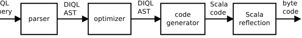
We present a new query language for DISC systems that is deeply embedded in Scala, called DIQL [20], and a query optimization framework that optimizes DIQL queries and translates them to Java byte code at compile-time. DIQL is designed to support multiple Scala-based APIs for distributed processing by abstracting their distributed data collections as a DataBag, which is a bag distributed across the worker nodes of a computer cluster. Currently, DIQL supports three Big Data platforms that provide different APIs and performance characteristics: Apache Spark, Apache Flink, and Twitter’s Cascading/Scalding. Unlike other query languages for DISC systems, DIQL can uniformly work on both distributed and in-memory collections using the same syntax. DIQL allows seamless mixing of native Scala code, which may contain UDF calls, with SQL-like query syntax, thus combining the flexibility of general-purpose programming languages with the declarativeness of database query languages.

DIQL queries may use any Scala pattern, may access any Scala variable, and may embed any Scala code without any marshaling. More importantly, DIQL queries can use the core Scala libraries and tools as well as user-defined classes without having to add any special declaration. This tight integration with Scala eliminates impedance mismatch, reduces program development time, and increases productivity, since it finds syntax and type errors at compile-time. DIQL

supports nested collections and hierarchical data, and allows query nesting at any place in a query. The query optimizer can find any possible join, including joins hidden across deeply nested queries, thus unnesting any form of query nesting. The DIQL algebra, which is based on monoid homomorphisms, can capture all the language features using a very small set of homomorphic operations. Monoids and monoid homomorphisms fully capture the functionality provided by current DSLs for DISC processing by directly supporting operations, such as group-by, order-by, aggregation, and joins on complex collections.

The intended users of DIQL are developers of DISC applications who 1) have a preference in declarative query languages, such as SQL, over the higher-order functional programming style used by DISC APIs, 2) want to use a full fledged query language that is tightly integrated with the host language, combining the flexibility of general-purpose programming languages with the declarativeness of database query languages, 3) want to express their applications in a platform-independent language and experiment with multiple DISC platforms without modifying their programs, 4) want to focus on the programming logic without having to add obscure and platform-dependent performance details to the code, and 5) want to achieve good performance by relying on a sophisticated query optimizer.

The contributions of this paper can be summarized as follows:

• We introduce a novel query language for large-scale distributed data analysis that is deeply embedded in Scala, called DIQL (Section 3). Unlike other DISC query languages, the query checking and code generation are done at compile-time. With DIQL, programmers can express complex data analysis tasks, such as PageRank, k-means clustering, and matrix factorization, using SQL-like syntax exclusively.

• We present an algebra for DISC, called the monoid algebra, which captures most features supported by current DISC frameworks (Section 4), and rules for translating DIQL queries to the monoid algebra (Section 5).

• We present algebraic transformations for deriving joins from nested queries that unnest nested queries of any form and any number of nesting levels, for pushing down predicates before joins, and for pruning unneeded data across operations, which generalize existing techniques (Section 6).

• We report on a prototype implementation of DIQL on three Big Data platforms, Spark, Flink, and

Scalding (Section 7) and explain how the DIQL type inference system is integrated with the Scala typing system using Scala’s compile-time reflection facilities and macros.

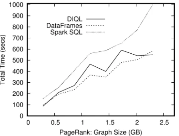
• We give evidence that DIQL has competitive performance relative to Spark DataFrames and Spark SQL by evaluating a simple nested query, a k-means clustering query, and a PageRank query (Section 9).

The DIQL syntax and some of the performance results have been presented in an earlier work [20]. The work reported in this paper extends our earlier work in four ways: 1) it fully describes the monoid algebra, which is used as the formal basis for our framework and as the target of query translation, 2) it gives the complete details of translating the DIQL syntax to algebraic terms, 3) it fully describes the query optimization framework, and 4) it provides more experimental results that give further evidence that our system has competitive performance relative to Spark DataFrames and Spark SQL.

2

R

ELATED

W

ORK

One of the earliest DISC frameworks was the Map-Reduce model, which was introduced by Google in 2004 [15]. The most popular Map-Reduce implementation is Apache Hadoop [5], an open-source project developed by Apache, which is used today by many companies to perform data analysis. Recent DISC systems go beyond Map-Reduce by maintaining dataset partitions in the memory of the worker nodes. Examples of such systems include Apache Spark [7] and Apache Flink [4]. There are also a number of higher-level languages that make Map-Reduce programming easier, such as HiveQL [36], PigLatin [30], SCOPE [13], DryadLINQ [37], and MRQL [18].

Apache Hive [36] provides a logical RDBMS environment on top of the Map-Reduce engine, well-suited for data warehousing. Using its high-level query language, HiveQL, users can write declarative queries, which are optimized and translated into Map-Reduce jobs that are executed using Hadoop. HiveQL does not handle nested collections uniformly: it uses SQL-like syntax for querying data sets but uses vector indexing for nested collections. Apache Pig [21] provides a user-friendly scripting language, called PigLatin [30], on top of Map-Reduce, which allows explicit filtering, map, join, and group-by operations. Programs in PigLatin are written as a sequence of steps (a dataflow), where each step carries out a single data transformation. This sequence of steps is not necessarily executed in that order; instead, when a store operation is encountered,

Pig optimizes the dataflow into a number of Map-Reduce barriers, which are executed as Map-Reduce jobs. Even though the PigLatin data model is nested, its language is less declarative than DIQL and does not support query nesting, but can simulate it using outer joins and coGroup.

In addition to the DSLs for data-intensive programming, there are some Scala-based APIs that simplify Map-Reduce programming, such as, Scalding [31], which is part of Twitter’s Cascading [12], Scrunch [32], which is a Scala wrapper for the Apache Crunch, and Scoobi. These APIs support higher-order operations, such as map and filter, which are very similar to those for Spark and Flink. Slick [33] integrates databases directly into Scala, allowing stored and remote data to be queried and processed in the same way as in-memory data, using ordinary Scala classes and collections. Summingbird [11] is an API-based distributed system that supports run-time optimization and can run on both Map-Reduce and Storm. Compared to Spark and Flink, the Summingbird API is intentionally more restrictive to facilitate optimization at run-time. The main shortcoming of all these API-based approaches is their inability to analyze the functional arguments of their high-level operations at run-time to do complex optimizations.

Vertex-centric graph-parallel programming is a new popular framework for large-scale graph processing. It was introduced by Google’s Pregel [28] but is now available by many open-source projects, such as Apache Giraph and Spark’s GraphX. Most of these frameworks are based on the Bulk Synchronous Parallelism (BSP) programming model. VERTEXICA[26] and Grail [16] provide the same vertex-centric interface as Pregel but, instead of a distributed file system, they use a relational database to store the graph and the exchanged messages across the BSP supersteps. Unlike Grail, which can run on a single server only, VERTEXICAcan run on multiple parallel machines connected to the same database server. Such configuration may not scale out very well because the centralized database may become the bottleneck of all the data traffic across the machines. Although DIQL is a general-purpose DISC query system, graph queries in DIQL are expressed using SQL-like syntax since graphs are captured as regular distributed collections. These queries are translated to distributed self-joins over the graph data. In [17], we proved that the monoid algebra can simulate any BSP computation (including vertex-centric parallel programs) efficiently, requiring the same amount of data shuffling as a typical BSP implementation.

DryadLINQ [37] is a programming model for large scale data-parallel computing that translates programs expressed in the LINQ programming model to Dryad,

which is a distributed execution engine for data-parallel applications. Like DIQL, LINQ is a statically strongly typed language and supports a declarative SQL-like syntax. Unlike DIQL, though, the LINQ query syntax is very limited and has limited support for query nesting. DryadLINQ allows programmers to provide manual hints to guide optimization. Currently, it performs static optimizations based on greedy heuristics only, but there are plans to implement cost-based optimizations in the future.

Apache Calcite [9] is a widely adopted relational query optimizer with a focus on flexibility, adaptivity, and extensibility. It is used for query optimization by a large number of open-source data-centric frameworks, including many DISC systems, such as Hive, Spark, Storm, and Flink. Although it can be adapted to work with many different platforms, its data model is purely relational with very little support for nested collections (it only supports indexing on inner collections), while its algebra is purely relational with no support for nested queries, such as, a query in a filter predicate.

There are some recent proposals for speeding up query plan interpretation in Volcano-style iterator-based query processing engines, used by many relational database systems, especially for main memory database systems for which CPU cost is important. Some of these systems are using a compiled execution engine to avoid the interpretation cost of algebraic expressions in a query plan. The HyPer database system [29], for example, translates algebraic expressions in a query to low-level LLVM code on the fly, so that the plan iterators are evaluated in a push-based fashion using loops. Instead of generating low-level code at once during the early stages of compilation, LegoBase [27] produces low-level C code in stages. It uses generative metaprogramming in Scala to take advantage of the type system of the language to check the correctness of the generated code, and to allow optimization and recompilation of code at various execution stages, including at run-time. Compared to our work, which also generates type-correct code at compile time, their focus is in the relational model and SQL, while ours is in a nested data model and complex nested queries, and their target is relational engines, while ours is DISC APIs.

Our work on embedded DSLs has been inspired by Emma [2, 3]. Unlike our work, Emma does not provide an SQL-like query syntax; instead, it uses Scala’s comprehensions to query datasets. These for-comprehensions are optimized and translated to abstract dataflows at compile-time, and these dataflows are evaluated at run-time using just-in-time code generation. Using the host language syntax for querying allows a deeper embedding of DSL code into the host language but it requires that the host language supports

meta-programming and provides a declarative syntax for querying collections, such as for-comprehensions. Furthermore, Scala’s for-comprehensions do not provide a declarative syntax for group-by. Emma’s core primitive for data processing is the fold operation over the union-representation of bags, which is equivalent to a bag homomorphism. The fold well-definedness conditions are similar to the preconditions for bag homomorphisms. Scala’s for-comprehensions are translated to monad comprehensions, which are desugared to monad operations, which, in turn, are expressed in terms of fold. Other non-monadic operations, such as aggregations, are expressed as folds. Emma also provides additional operations, such as groupBy and join, but does not provide algebraic operations for sorting, outer-join (needed for non-trivial query unnesting), and repetition (needed for iterative workflows). Unlike DIQL, Emma does not provide general methods to convert nested correlated queries to joins, except for simple nested queries in which the domain of a generator qualifier is another comprehension.

The syntax and semantics of DIQL have been influenced by previous work on list comprehensions with order-by and group-by [39]. Monoid homomorphisms and monoid comprehensions were first introduced as a formalism for OO queries in [19] and later as a query algebra for MRQL [18]. Our monoid algebra extends these algebras to include group-by, coGroup, and order-by operations. Many other algebras and calculi are based on monads and monad comprehensions. Monad comprehensions have a number of limitations, such as inability to capture grouping and sorting on bags. Monads also require various extensions to capture aggregations and heterogeneous operations, such as, converting a list to a bag. Monoids on the other hand can naturally capture aggregations, ordering, and group-by without any extension. Many other algebras and calculi in related work are based on monad comprehensions [38]. In an earlier work [17], we have shown that monoid comprehensions are a better formal basis for practical DISC query languages than monad comprehensions.

The syntax of DIQL is based on the syntax of MRQL [18], which is a query language for large-scale, distributed data analysis. The design of MRQL, in turn, has been influenced by XQuery and ODMG OQL, although it uses SQL-like syntax. Unlike MRQL, DIQL allows general Scala patterns and expressions in a query, it is more tightly integrated with the host language, and it is optimized and compiled to byte code at compile-time, instead of run-time.

3

DIQL:

A

D

ATA

-I

NTENSIVE

Q

UERY

L

ANGUAGE

This section presents the detailed syntax of DIQL. As an example of a DIQL query evaluated on Spark, consider matrix multiplication. We can represent a sparse matrix M as a distributed collection of type RDD[(Double,Int,Int)] in Spark, so that a triple (v, i, j)

in this collection represents the matrix element v =

Mij. Then the matrix multiplication between two sparse matricesX andY can be expressed as follows in DIQL: Query A:

select(+/z, i, j)

from(x, i, k)<−X, (y, k , j) <−Y, z=x∗y wherek==k

group by(i, j)

whereX andY are embedded Scala variables of type RDD[(Double,Int,Int)]. This query retrieves the values Xik∈XandYkj∈Y for alli, j, k, and setsz=Xik∗

Ykj. The group-by operation lifts each pattern variable defined before the group-by (except the group-by keys) from some type t to a bag of t, indicating that each such variable must now contain all the values associated with the same group-by key value. Consequently, after we group the values by the matrix indexesiandj, the variablezis lifted to a bag of numerical valuesXik∗Ykj, for allk. Hence, the aggregation+/zwill sum up all the values in the bag z, deriving P

kXik∗ Ykj for the ij element of the resulting matrix.

As another example, consider the matrix addition between the two sparse matrices X and Y. Given that missing values in sparse matrices correspond to zero values, matrix addition should be expressed in a relational query as a full outer join, not an inner join. Instead, this operation is specified as follows in DIQL:

Query B:

select(+/(x++y), i, j)

from(x, i, j) <−Xgroup by(i, j)

from(y, i , j ) <−Y group by(i , j )

Each of the two group-by clauses in this query groups only the variables in their associated from-clause: X values are grouped by(i, j)andY values are grouped by

(i , j ). Furthermore, the two group keys are implicitly set to be equal, (i, j) = (i , j ). That is, after X is grouped by (i, j) and Y is grouped by (i , j ), the resulting grouped datasets are joined over their group-by key. That is, this query is equivalent to a coGroup operation found in many DISC APIs. The semantics of this double group-by query is very similar to that of the single group-by: The first (resp. second) group-by lifts the variablex(resp.y) to a bag ofDouble, which may

be either empty or singleton. That is, the concatenation x++y may contain one or two values, which are added together in+/(x++y). In contrast to a relational outer join, this query does not introduce any null values since it is equivalent to a coGroup operation.

Many emerging Scala-based APIs for distributed processing, such as the Scala-based Hadoop Map-Reduce frameworks Scalding and Scrunch, and the Map-Reduce alternatives Spark and Flink, are based on distributed collections that resemble regular Scala data collections as they support similar methods. Many Big Data analysis applications need to work on nested collections, because, unlike relational databases, they need to analyze data in their native format, as they become available, without having to normalize these data into flat relations first. While outer collections need to be distributed in order to be processed in parallel, the inner sub-collections must be stored in memory and processed as regular Scala collections. Processing both kinds of collections, distributed and in-memory, using the same syntax or API simplifies program development considerably. The DIQL syntax treats distributed and in-memory collections in the same way, although DIQL optimizes and compiles the operations on these collections differently. The DIQL data model supports four collection types: a bag, which is an unordered collection (a multiset) of values stored in memory, a DataBag, which is a bag distributed across the worker nodes of a computer cluster, a list, which is an ordered collection of values stored in memory, and a DataList, which is an ordered DataBag.

For example, let R and S be two distributed collections in Spark of type RDD[(Long,Long)] and RDD[(Long,Long,Long)], respectively. Then the following Scala code fragment that contains a DIQL query joins the datasetsRandSusing a nested query:

Query C: q(””” select( x, +/(selectb from(a,b, ) <−S wherea==y) ) from(x,y) <−R ”””)

In SQL, this query would have been written as a left-outer join betweenRandS, followed by a group-by with an aggregation. The DIQL syntax can be embedded in a Scala program using the Scala macroq(” ” ” ... ” ” ”), which is optimized and compiled to byte code at compile-time. This byte code in turn is embedded in the byte code generated by the rest of the Scala program. That is, all type errors in the DIQL queries are captured at compile-time. Furthermore, a query can see any active Scala declaration in the current Scala scope, including

Table 1: The DIQL syntax

pattern: p ::= any Scala pattern, including a refutable pattern

qualifier: q ::= p <−e generator over a dataset

| p <−− e generator over a small dataset

| p = e binding

qualifiers: q ::= q1, . . . , qn sequence of qualifiers

aggregation: ⊕ ::= +| ∗ |&&| || |count|avg|min|max| . . . expression: e ::= any Scala functional expression

| select[distinct]e0fromq[whereep] select-query

[group byp[ :e] [cg] [havingeh] ] [order byes]

| repeatp = estepe0_[wheree

p] [limitn] repetition

| someq: ep existential quantification

| allq: ep universal quantification

| letp=e1ine2 let-binding

| e1opre2 opris a set operation: union,

intersect, minus, or member

| ⊕/e aggregation

co-group: cg ::= fromq[whereep]group byp[ :e] the right branch of a coGroup

the results of other queries if they have been assigned to Scala variables.

The DIQL syntax is Scala syntax extended with the DIQL select-query syntax (among other things), as is described in Table 1. It uses a purely functional subset of Scala, which intentionally excludes blocks, declarations, iterations (such as while loops), and assignments, because imperative features are hard to optimize. Instead, DIQL provides special syntax for let-binding and iteration. DIQL queries can use any Scala pattern to pattern-match and deconstruct data. The qualifier(x,y)<−Rin Query C traverses the datasetR one element at a time and matches the element with the Scala pattern (x,y), which binds the pattern variablesx andyto the first and second components of the matched element. That is,xandyhave typeLong. The qualifier (a,b, )<−Sin the inner select-query, on the other hand, traverses the datasetSone element at a time and matches the element with the Scala pattern(a,b, ), which binds the pattern variables a and b to the first and second components of the matched element. The underscore in the pattern matches any value but the matched value is ignored. That is, Query C joins R withS on their second components using a nested query so that the query result will have exactly one value for each element

inR even when this element has no match in S. The aggregation +/(. . . ) in the outer query sums up all the values returned by the inner query. The query result is of typeRDD[(Long,Long)]and can be embedded in any place in a Scala program where a value of this type is expected.

The Scala code for Query C generated by the DIQL compiler is equivalent to a Spark cogroup method call that joins theRwithS:

R.map{caser@(x,y)=>(y,r)}

.cogroup( S.map{cases@(a,b, )=>(b,s)}) .flatMap{case(k,( rr ,ss))

=>rr.map{case(x,y)

=>( x, ss.map{case(a,b, )=>b}

.reduce( + ) ) } } where the Scala pattern binderx@pmatches a value with the patternpand binds xto that value. The mapcalls onRandSprepare these datasets for the cogroupjoin by selecting the second component of their tuples as the join key. The flatMapcall aftercogroup computes the query result from the sequencesrrandss of all values fromRandSthat are joined over the same keyk. This query cannot be expressed using a Sparkjoinoperation because it will loose all values fromRthat are not joined with any value fromS.

class that represents a graph node:

case classNode ( id: Long, adjacent: List [Long] )

whereadjacentcontains theids of the node’s neighbors. Then, a graph in Spark can be represented as a distributed collection of type RDD[Node]. Note that the inner collection of typeList[Long]is an in-memory collection since it conforms to the class Traversable. The following DIQL query constructs the graph RDD from a text file stored in HDFS and then transforms this graph so that each node is linked with the neighbors of its neighbors:

Query D:

let graph =selectNode( id = n, adjacent = ns )

fromline <−sc.textFile(”graph.txt ”), n :: ns = line . split (” , ”). toList

.map( .toLong)

in selectNode( x, ++/ys )

fromNode(x,xs)<−graph, a<−xs,

Node(y,ys)<−graph

wherey == agroup byx

In the previous DIQL query, the let-binding binds the new variable graph to an RDD of type RDD[Node], which contains the graph nodes read from HDFS, mixing DIQL syntax with Spark API methods. The DIQL type-checker will infer that the type ofsc.textFile(”graph.txt”) isRDD[String], and, hence, the type of the query variable lineisString. Based on this information, the DIQL type-checker will infer that the type of n:ns in the pattern of the let-binding is List[Long], which is a Traversable collection. The select-query in the body of the let-binding expresses a self-join overgraph followed by a group-by. The pattern Node(x,xs) matches one graph element at a time (aNode) and bindsxto the node id and xsto the adjacent list of the node. Hence, the domain of the second qualifiera<−xsis an in-memory collection of type List[Long], making ‘a’ a variable of typeLong. The graph is traversed a second time and its elements are matched with Node(y,ys). Thus, this select-query traverses two distributed and one in-memory collections. In general, as we can see in Table 1, a select-query may have multiple qualifiers in the ‘from’ clause of the query. A qualifierp <−e, whereeis a DIQL expression that returns a data collection and pis a Scala pattern (which can be refutable - i.e., it may fail to match), iterates over the collection and, each time, the current element of the collection is pattern-matched with p, which, if the match succeeds, binds the pattern variables in pto the matched components of the element. The qualifierp <−−edoes the same iteration asp <−ebut it also gives a hint to the DIQL optimizer that the collection eis small (can fit in the memory of a worker node) so that the optimizer may consider using a broadcast join. The binding p = e pattern-matches the pattern pwith the

value returned byeand, if the match succeeds, binds the pattern variables inpto the matched components of the valuee. The variables introduced by a qualifier pattern can only be accessed by the remaining qualifiers and the rest of the query. The group-by syntax is explained next. Unlike other query languages, patterns are essential to the DIQL group-by semantics; they fully determine which parts of the data are lifted to collections after the group-by operation. The group-by clause has syntax

group byp:e. It groups the query result by the key returned by the expressione. Ifeis missing, it is taken to be equal top. For each group-by result, the patternpis pattern-matched with the key, while any pattern variable in the query that does not occur inpis lifted to an in-memory collection that contains all the values of this pattern variable associated with this group-by result. For our Query D, the query result is grouped byx, which is both the patternpand the group-by expressione. After group-by, all pattern variables in the query except x, namelyxs,y, andys, are lifted to collections.

In particular, ys of type List[Long] is lifted to a collection of type List[List[Long]], which is a list that contains allys associated with a particular value of the group-by keyx. Thus, the aggregation++/yswill merge all values in ys using the list append operation, ++, yielding aList[Long]. In general, the DIQL syntax⊕/e can use any Scala operation⊕of type(T, T) → T to reduce a collection of T (distributed or in-memory) to a value T. The same syntax is used for the avg and count operations over a collection, e.g.,avg/sreturns the average value of the collection of numerical values s. The existential quantificationsome q : ep is syntactic sugar for||/(select ep from q), that is, it evaluates the predicateep on each element in the collection resulted from the qualifiersqand returns true if at least one result is true. Universal quantification does a similar operation using the aggregator&&, that is, it returns true if all the results of the predicateepare true.

The Scala code for the second select-query of Query D generated by the DIQL compiler is equivalent to a call to the Spark cogroup method that joins thegraphwith itself, followed by a reduceByKey:

graph.flatMap{casen@Node(x,xs)=>xs.map{a=>(a,n)}}

.cogroup(graph.map{casem@Node(y,ys)=>(y,m)}) .flatMap{case( ,( ns,ms))

=>ns.flatMap{caseNode(x,xs)

=>xs.flatMap{a=>ms.map{caseNode(y,ys) =>(x,ys)} } } }

.reduceByKey( ++ ).map{case(x,s)=>Node(x,s)} The co-group clause cg in Table 1 represents the right branch of a coGroup operation (the left branch is the first group-by clause). As explained in Query B (matrix addition), each of the two group-by clauses lifts the pattern variables in their associated from-clause

qualifiers and joins the results on their group-by keys. Hence, the rest of the query can access the group-by keys from the group-by clauses and the lifted pattern variables from both from-clauses. The co-group clause captures any coGroup operation, which is more general than a join. That is, using the co-group syntax one can capture any inner and outer join without introducing any null values and without requiring 3-value logic to evaluate conditions.

The order-by clause of a select-query has syntax order byes, which sorts the query result by the sorting key es. One may use the pre-defined method desc to coerce a value to an instance of the class Inv, which inverts the total order of an Ordered class from≤to≥. For example,

selectp

fromp@(x,y)<−S

order by( x desc, y )

sorts the query result by major orderx(descending) and minor ordery(ascending).

Finally, to capture data analysis algorithms that require iteration, such as data clustering and PageRank, DIQL provides a general syntax for repetition:

repeatp = estepe0whereeplimitn which does the assignmentp = e0 repeatedly, starting withp =e, until either the conditionep becomes false or the number of iterations has reached the limitn. In Scala, this is equivalent to the following code, wherex is the result of the repetition:

varx=e for(i <−0ton)

xmatch{casepifep => x=e0 case => break}

As we can see, the variables inpcan be accessed ine0, allowing us to calculate new variable bindings from the previous ones. The type of the result of the repetition can be anything, including a tuple with distributed and in-memory collections, counters, etc.

For example, the following query implements the k-means clustering algorithm by repeatedly derivingknew centroids from the previous ones:

Query E:

repeatcentroids = Array( ... )

step selectPoint( avg/x,avg/y )

fromp@Point(x,y)<−points

group byk: (selectc fromc<−centroids

order bydistance(c,p) ). head

limit 10

wherepointsis a distributed dataset of points on the X-Y plane of typeRDD[Point], wherePointis the Scala class:

case classPoint ( X: Double, Y: Double )

centroids is the current set of centroids (k cluster centers), anddistanceis a Scala method that calculates the Euclidean distance between two points. The initial value ofcentroids(the... value) is an array of kinitial centroids (omitted here). The inner select-query in the group-by clause assigns the closest centroid to a pointp. The outer select-query in the repeat step clusters the data points by their closest centroid, and, for each cluster, a new centroid is calculated from the average values of its points. That is, the group-by query generateskgroups, one for each centroid.

For a group associated with a centroidc, the variable p is lifted to a Iterable[Point] that contains the points closest toc, whilexandy are lifted toIterable[Double] collections that contain the X- and Y-coordinates of these points. DIQL implements this query in Spark as a flatMap over points followed by a reduceByKey. The Spark reduceByKey operation does not materialize the Iterable[Double] collections in memory; instead, it calculates the avg aggregations in a stream-like fashion. DIQL caches the result of the repeat step, which is an RDD, into an array, because it has decided thatcentroids should be stored in an array (like its initial value). Furthermore, the flatMap functional argument accesses the centroids array as a broadcast variable, which is broadcast to all worker nodes before the flatMap.

4

T

HE

M

ONOID

A

LGEBRA

The main goal of our work is to translate DIQL queries to efficient programs that can run on various DISC platforms. Experience with the relational database technology has shown that this translation process can be simplified if we first translate the queries to an algebraic form that is equivalent to the query and then translate the algebraic form to code consisting of calls to API operations supported by the underlying DISC platform.

Our algebra consists of a very small set of operations that capture all the DIQL features and can be translated to efficient byte code that uses the Scala-based APIs of DISC platforms. We intentionally use only one higher-order homomorphic operation in our algebra, namely flatMap, to simplify normalization and optimization of algebraic terms. The flatMap operation captures data parallelism, where each processing node evaluates the same code (the flatMap functional argument) in parallel on its own data partition. The groupBy operation, on the other hand, re-shuffles the data across the processing nodes based on the group-by key, so that data with the same key are sent to the same processing node. The coGroup operation is a groupBy over two collections, so that data with the same key from both collections

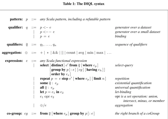
Table 2: Some collection monoids ~ T(α) 1_~ U~(x) properties list ++ [α] [ ] [x] bag ] {{α}} {{ }} {{x}} commutative set ∪ {α} { } {x} commutative and idempotent

are sent to the same node to be joined. By moving all computations to flatMap, our algebra detaches data distribution (specified by groupBy and coGroup) from parallel data processing (specified by flatMap). This separation simplifies program optimization considerably. For example, as we will see in Section 6.2, query unnesting can be done using just one rule, because there is only one place where a nested query can occur: at the flatMap functional argument.

This section extends our previous work on the monoid algebra [17] by improving the semantics of some operations (such as, orderBy and repeat) and introducing more operations (such as, the cross product).

Collection monoids and homomorphisms. In abstract algebra, a monoid is an algebraic structure equipped with a single associative binary operation and a single identity element. More formally, given a setS, a binary operator⊗fromS ×S toS, and an element e∈S, the structure(S,⊗, e)is called a monoid if⊗is associative and has an identitye:

x⊗(y⊗z) = (x⊗y)⊗z for allx, y, z∈S x⊗e=x=e⊗x for allx∈S

Monoids may satisfy additional algebraic laws. The monoid(S,⊗, e)is commutative ifx⊗y =y⊗x, for all x, y ∈ S. It is idempotent if x⊗x = x, for all x∈ S. Given that a monoid(S,⊗, e)can be identified by its operation⊗, it is simply referred to as⊗, with1⊗ to denote its identitye. Given two monoids⊗and⊕, a monoid homomorphismfrom⊗to⊕is a functionHthat respects the monoid structure:

H(X⊗Y) =H(X) ⊕H(Y)

H(1⊗) =1⊕

A data collection, such as a list, a set, or a bag, of type T(α), for some typeα, can be captured as acollection monoid ~, which is a monoid equipped with a unit injection function_U~of typeα→T(α). Table 2 shows some well-known collection types captured as collection monoids.

For example, {{1}} ] {{2}} ] {{1}}constructs the bag {{1,2,1}}. A collection homomorphism is a monoid homomorphismH(⊕, f)from a collection monoid⊗to

a monoid⊕defined as follows, forH =H(⊕, f): H(X⊗Y) = H(X) ⊕H(Y)

H(U⊗(x)) = f(x)

H(1⊗) = 1⊕

For example, H(+, λx.1)X over the bag X returns the number of elements in X. Not all collection homomorphisms are well-behaved; some may actually lead to contradictions. In general, a collection homomorphism from a collection monoid⊗to a monoid ⊕ is well-behaved if ⊕ satisfies all the laws that ⊗ does (the laws in our case are commutativity and idempotence). For example, converting a list to a bag is well-behaved, while converting a bag to a list and set cardinality are not. For example, set cardinality would have led to the contradiction: 2 = H(+, λx.1) ({a} ∪ {a}) =H(+, λx.1){a}= 1.

All unary operations in the monoid algebra are collection homomorphisms. To capture binary equi-joins, we define binary functions that are homomorphic on both inputs. Abinary homomorphism H from the collection monoids⊕and⊗to the monoidsatisfies, for allX,X0,Y, andY0:

H(X⊕X0, Y ⊗Y0) =H(X, Y) H(X0, Y0)

One such function is

H(X, Y) =H(, fx)(X) H(, fy)(Y)

for some functionsfxandfythat satisfy:

fx(x)fy(y) = fy(y)fx(x) for allxandy The Monoid Algebra. The DIQL data model supports four collection types: a bag, which is an unordered collection (a multiset) of values stored in memory, a DataBag, which is a bag distributed across the worker nodes of a computer cluster, a list, which is an ordered collection in memory, and a DataList, which is an ordered DataBag. Both bags and lists are implemented as Scala Traversable collections, while both DataBags and DataLists are implemented as RDDs in Spark, DataSets in Flink, and TypedPipes in Scalding. The DIQL type inference engine can distinguish bags from lists and DataBags from DataLists by just looking at the algebraic operations: the orderBy operation always returns a list or a DataList, while the order is destroyed by all DIQL algebraic operations except flatMap. To simplify the presentation of our algebra, we present only one variation of each operation, namely one that works on bags. The flatMap, for example, has many variations: from a bag to a bag using a functional that returns a bag, from a list to list using a functional that returns a

list, from a DataBag to a DataBag using a functional that returns a bag, etc, but some combinations are not permitted as they are not well-behaved, such as a flatMap from a bag to a list.

The flatMap operation.The first operation, flatMap, generalizes the select, project, join, cross, and unnest operations of the nested relational algebra. Given two arbitrary types α and β, the operation flatMap(f, X)

over a bag X of type {{α}} applies the function f of typeα→ {{β}}to each element ofX, yielding one bag for each element, and then merges these bags to form a single bag of type {{β}}. It is expressed as follows as a collection homomorphism from the monoid]to the monoid]:

flatMap(f, X) _, H(], f)X which is equivalent to the following equations:

flatMap(f, X]Y) = flatMap(f, X) ]flatMap(f, Y) flatMap(f,{{a}}) = f(a)

flatMap(f,{{ }}) = {{ }}

Many common distributed queries can be written using flatMaps, including the equi-joinX ./pY:

flatMap(λx.flatMap(λy.ifp(x, y)then{{(x, y)}} else{{ }}, Y),

X)

The flatMap operation is the only higher-order homomorphic operation in the monoid algebra. Its functional argument can be any Scala function, including a partial function with a refutable pattern. In that case, the second flatMap equation becomes a pattern matching that returns an empty bag if the refutable pattern fails to match.

flatMap(λp. e,{{a}})

=amatch{casep => e; case => {{ }} } whereλp. eis an anonymous function, expressed asp⇒

ein Scala, where pis a Scala pattern and eis a Scala expression.

The groupBy operation. Given a type κ that supports value equality (=), a type α, and a bagX of type {{(κ, α)}}, the operation groupBy(X) groups the elements ofX by their first component (the group-by key) and returns a bag of type{{(κ,{{α}})}}(a key-value map, also known as an indexed set). It can be expressed as follows as a collection homomorphism:

groupBy(X) _, H(m, λ(k, v).{{(k,{{v}})}})X

which is equivalent to the following equations:

groupBy(X]Y) = groupBy(X) m groupBy(Y) groupBy({{(k, v)}}) = {{(k,{{v}})}}

groupBy({{ }}) = {{ }}

The monoidm, calledindexed set union, is a full outer join that merges groups associated with the same key using bag union. More specifically,X mY is a full outer join betweenX andY that can be defined as follows using a set-former notation on bags:

X m Y

= {(k, a]b)|||(k, a)∈X,(k0, b)∈Y, k=k0} ] {(k, a)|||(k, a)∈X,∀(k0, b)∈Y :k0 6=k} ] {(k, b)|||(k, b)∈Y,∀(k0, a)∈X:k06=k} The first term joins X and Y on the group-by key and unions together the groups associated with the same key, the second term returns the elements of X not joined with Y, and the third term returns the elements of Y not joined with X. For example, groupBy({{(1,“a”),(2,“b”),(1,“c”)}})

returns{{(1,{{“a”,“c”}}),(2,{{“b”}})}}.

The orderBy operation.Given a typeκthat supports a total order (≤), a typeα, and a bagXof type{{(κ, α)}}, the operationorderBy(X)returns a list of type [(κ, α)] sorted by the order-by keyκ. It is expressed as follows as a collection homomorphism:

orderBy(X) _, H(⇑, λ(k, v).[(k, v)])X which is equivalent to the following equations:

orderBy(X]Y) = orderBy(X) ⇑ orderBy(Y) orderBy({{(k, v)}}) = [(k, v)]

orderBy({{ }}) = [ ]

The monoid ⇑ merges two sorted sequences of type [(κ, α)] to create a new sorted sequence. It can be expressed as follows using a set-former notation on lists (list comprehensions): (X1++X2)⇑Y = X1⇑(X2⇑Y) [(k, v)]⇑Y = [(k0, w)|||(k0, w)∈Y, k0 < k] ++[(k, v)] ++[(k0, w)|||(k0, w)∈Y, k0≥k] [ ]⇑Y = Y

The second equation inserts the pair(k, v)into the sorted listY, deriving a sorted list.

The reduce operation. Aggregations are captured by the collection homomorphismreduce(⊕, X), which aggregates a bagXof type{{α}}using the non-collection monoid⊕of typeα:

For example,reduce(+,{{1,2,3}}) = 6.

The coGroup operation. Although general joins and cross products can be expressed using nested flatMaps, we provide a binary homomorphism that captures lossless equi-joins and outer joins. The operation coGroup(X, Y) between a bag X of type {{(κ, α)}}and a bagY of type{{(κ, β)}}over their first component of typeκ(the join key) returns a bag of type {{(κ,({{α}},{{β}}))}}. It is homomorphic on both inputs as it satisfies the law:

coGroup(X1]X2, Y1]Y2)

= coGroup(X1, Y1) l coGroup(X2, Y2)

where the monoidlmerges pairs of bags associated with the same key.

X l Y = {(k,(a1]b1, a2]b2)) |||(k,(a1, a2))∈X,(k 0 ,(b1, b2))∈Y, k=k 0 } ] {(k, p)|||(k, p)∈X,∀(k0, q)∈Y :k06=k} ] {(k, q)|||(k, q)∈Y,∀(k0, p)∈X:k06=k}

For example, coGroup( {{(1,10),(2,20),(1,30)}},

{{(1,40),(2,50),(3,60)}} ) ={{(1,({{10,30}},{{40}})),

(2,({{20}},{{50}})),(3,({{ }},{{60}}))}}.

The cross product operation, cross(X, Y) is the Cartesian product betweenXof type{{α}}andY of type {{β}}that returns{{(α, β)}}. Unlike coGroup, it is not a monoid homomorphism:

cross(X1]X2, Y1]Y2)

= cross(X1, Y1) ] cross(X1, Y2) ]cross(X2, Y1)] cross(X2, Y2)

The repeat operation. Given a value X of type α, a function f of type α→α, a predicate p of type α→boolean, and a counter n, the operation

repeat(f, p, n, X)returns a value of typeα. It is defined as follows:

repeat(f, p, n, X) _, ifn≤0 ∨ ¬p(X) thenX

else repeat(f, p, n−1, f(X))

The repetition stops when the number of remaining repetitions is zero or the result value fails to satisfy the conditionp.

5

T

RANSLATION OF

DIQL

TO THE

M

ONOID

A

LGEBRA

Table 3 presents the rules for translating DIQL queries to the monoid algebra. The form QJeKtranslates the DIQL syntax of e (defined in Table 1) to the monoid algebra. The notationλp.e, wherepis a Scala pattern, is an anonymous functionfdefined asf(p) =e. Although

the rules in Table 3 translate join queries to nested flatMaps, in Section 6.2, we present a general method for deriving joins from nested flatMaps.

The order that select-queries are translated in Table 3 is as follows: the distinct clause is translated first, then the order-by clause, then the group-by/having clauses, then the ‘from’ clause (the query qualifiers), then the ‘where’ clause, and finally the select header (the query result). Rule (1) translates a distinct query to a group-by that removes duplicates group-by grouping the query result values by the entire value. Rule (2) translates an order-by query to an orderBy operation.

Rules (3) and (4) translate group-by queries. Recall that, after group-by, every pattern variable in a query except the group-by pattern variables, are lifted to a collection of values to contain all bindings of this variable associated with a group. To specify these bindings, we use the notationV_qpto denote the flat tuple that contains all pattern variables in the sequence of qualifiersq that do not appear in the group-by pattern p. It is defined as V_qp = (v1, . . . , vn) (the order of v1, . . . , vnis unimportant), wherevi∈(VJqK− PJpK) andVis defined as follows:

VJp <−e, qK = PJpK∪ VJqK

VJp <−− e, qK = PJpK∪ VJqK

VJp=e, qK = PJpK∪ VJqK wherePJpKis the set of pattern variables in the pattern p. As a simplification, we lift only the variables that are accessed by the rest of the query, since all others are ignored. The queryselect (e,V_qp)from qin Rules (3) and (4) is the query before the group-by operation that returns a collection of pairs that consist of the group-by key and the non-group-group-by variables V_qp. Hence, after groupBy, the non-group-by variables are grouped into a collection to be used by the rest of the query. The operation lift((v1, . . . , vn), s, e), where s is the collection that contains the values of the non-group-by variables in the current group, lifts each variablevito a collection by rebinding it to a collection derived froms asflatMap(λ(v1, . . . , vn).{{vi}}, s).

Rule (5) translates a generatorp <−eto a flatMap. Rule (6) is similar, but embeds the annotation ‘small’ (which is the identity operation), to be used by the optimizer as a hint about the collection size. Rule (7) gives the translation of a let-binding for an irrefutable patternp. For a refutablep, the translation is:

QJeKmatch{casep => QJselectefromqK

case => {{ }} }

Rules (8) and (9) are the last rules to be applied when all qualifiers in the query have been translated, and hence, the ‘from’ clause is empty. Rule (8)

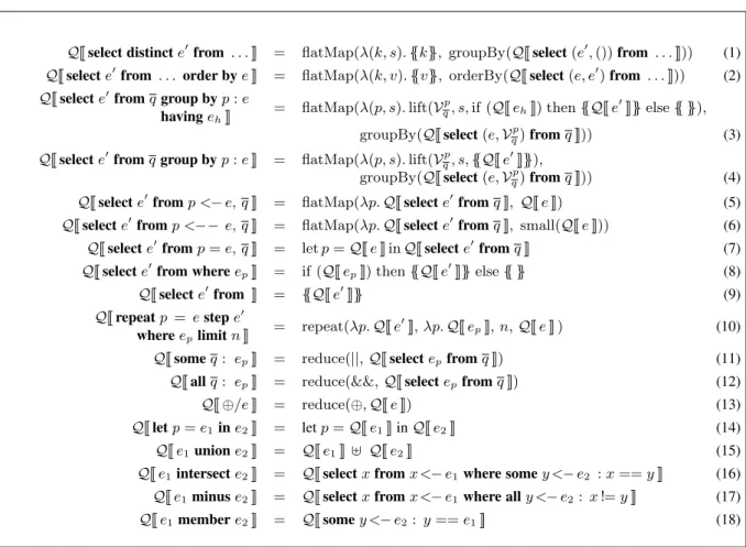
Table 3: DIQL query translation rules

QJselect distincte0from . . .K = flatMap(λ(k, s).{{k}}, groupBy(QJselect(e0,())from . . .K)) (1)

QJselecte0from . . . order byeK = flatMap(λ(k, v).{{v}}, orderBy(QJselect(e, e0)from . . .K)) (2)

QJselecte0fromqgroup byp:e

havingehK = flatMap(λ(p, s).lift(V p

q, s,if (QJehK) then{{QJe0K}}else{{ }}), groupBy(QJselect(e,Vp

q)fromqK)) (3) QJselecte0fromqgroup byp:eK = flatMap(λ(p, s).lift(Vp

q, s,{{QJe

0_K

}}),

groupBy(QJselect(e,Vp

q)fromqK)) (4) QJselecte0fromp <−e, qK = flatMap(λp.QJselecte0fromqK, QJeK) (5)

QJselecte0fromp <−− e, qK = flatMap(λp.QJselecte0fromqK, small(QJeK)) (6)

QJselecte0fromp=e, qK = letp=QJeKinQJselecte0fromqK (7)

QJselecte0from whereepK = if (QJepK) then{{QJe0K}}else{{ }} (8)

QJselecte0from K = {{QJe0K}} (9)

QJrepeatp =estepe0

whereeplimitnK = repeat(λp.QJe

0_K

, λp.QJepK, n,QJeK) (10)

QJsomeq: epK = reduce(||,QJselectepfromqK) (11)

QJallq: epK = reduce(&&,QJselectepfromqK) (12)

QJ⊕/eK = reduce(⊕,QJeK) (13)

QJletp=e1ine2K = letp=QJe1KinQJe2K (14)

QJe1unione2K = QJe1K] QJe2K (15) QJe1intersecte2K = QJselectxfromx <−e1where somey <−e2 :x==yK (16) QJe1minuse2K = QJselectxfromx <−e1where ally <−e2: x!=yK (17) QJe1membere2K = QJsomey <−e2: y==e1K (18)

translates the ‘where’ clause of a query with an empty ‘from’ clause. Rule (10) translates the repeat syntax to the repeat operation. Rules (11) through (13) translate accumulations to reduce operations. Rule (14) translates a DIQL let-binding to a Scala let-binding. Finally, Rules (15) through (18) translate bag union, bag intersection, bag difference, and bag membership to a select query.

For example, in Query A (matrix multiplication), the only variable that needs to be lifted after group-by isz, since it is the only one used by the rest of the query. That is,V_qp = (z). Hence, the matrix multiplication is translated as follows:

QJselect(+/z, i, j)

from(x, i, k)<−X, (y, k , j)<−Y, z=x∗y wherek==k group by(i, j)K

=flatMap(λ((i, j), s).letz=flatMap(λz.{{z}}, s)

in{{QJ(+/z, i, j)K}} groupBy(join))

=flatMap(λ((i, j), s).{{(reduce(+, s), i, j)}}, groupBy(join))

where join is: QJselect((i, j), z) from(x, i, k)<−X, (y, k , j)<−Y, z=x∗y wherek==k K =flatMap(λ(x, i, k). flatMap(λ(y, k , j). letz=x∗y in if(k==k )then{{((i, j), z)}} else{{ }}, Y), X) =flatMap(λ(x, i, k). flatMap(λ(y, k , j). if(k==k)then{{((i, j), x∗y)}} else{{ }}, Y), X)

We will see in Section 6.2 that join-like queries such as this, expressed with nested flatMaps, are optimized to coGroups.

Finally, Table 3 does not show the rules for translating a co-group clausecgdefined in Table 1. These double

group-by clauses are translating to coGroups using the following rule: QJselecte0_fromq 1group byp1:e1 fromq2group byp2:e2K = flatMap(λ((p1, p2),(s1, s2)). lift(Vp1 q1, s1,lift(V p2 q2, s2,{{QJe 0_K}})), coGroup(QJselect(e1,Vp1

q1)fromq1K,

QJselect(e2,Vp2

q2)fromq2K))

For example, for Query B (matrix addition), we have Vp1 q1 = (x)andV p2 q2 = (y). Consequently, Query B is translated as follows: flatMap(λ(((x, i, j),(y, i , j )),(s1, s2)). letx=flatMap(λ(x, i, j).{{x}}, s1), y=flatMap(λ(y, i , j ).{{y}}, s2) in{{(+/(x++y), i, j)}}, coGroup(A, B))

whereA=QJselect((i, j), x)from(x, i, j) <−XK

= flatMap(λ(x, i, j).{{((i, j), x)}}, X)and, similarly, B = QJselect ((i , j ), y) from (y, i , j ) <− Y K

=flatMap(λ(y, i , j ).{{((i , j ), y)}}, Y).

6

Q

UERY

O

PTIMIZATION

Given a DIQL query, our goal is to translate it into an algebraic form that can be evaluated efficiently in a DISC platform. Current database technology has already addressed this problem in the context of relational databases. The DIQL data model and algebra though are richer than those of a relational system, requiring more general optimization techniques. The relational algebra, for instance, as well as the algebraic operators used by current relational engines, such as Calcite [9], cannot express nested queries, such as a query inside a selection predicate, thus requiring the query translator to unnest queries using source-to-source transformations before the queries are translated to algebraic terms. This limitation may discourage language designers to support nested queries, although they are very common in DISC data analysis (for example, the k-means clustering query (Query E)).

Currently, our optimizations are not based on any cost model; instead, they are heuristics that take into account the hints provided by the user, such as using

a <-- qualifier to traverse a small dataset. That is,

our framework tries to identify all possible joins and convert them to broadcast joins if they are over a small dataset, but currently, it does not optimize the join order. In this section, we present the normalization rules that put DIQL terms to a canonical form (Section 6.1), a general method for query unnesting (Section 6.2), pushing down predicates (Section 6.3), and column pruning (Section 6.4).

6.1

Query Simplification

Cascaded flatMaps can be fused into a single nested flatMap using the following law that is well-known in functional PLs:

flatMap(f,flatMap(g, S))

→flatMap(λx.flatMap(f, g(x)), S) (19) If S is a distributed dataset, this normalization rule reduces the number of required distributed operations from two to one and eliminates redundant operations if we apply further optimizations to the inner flatMap. It generalizes well-known algebraic laws in relational algebra, such as fusing two cascaded selections into one. If we apply this transformation repeatedly, any algebraic term can be normalized into a tree of groupBy, coGroup, and cross operations with a single flatMap between each pair of these operations. There are many other standard normalization rules, such as projecting over a tuple, (e1, . . . , en). i = ei, and rules that are derived directly from the operator’s definition, such as

flatMap(f,{{a}}) =f(a).

6.2

Deriving Joins and Unnesting Queries

The translation rules from the DIQL syntax to the monoid algebra, presented in Section 5, translate join-like queries to nested flatMaps, instead of coGroups. In this section, we present a general method for identifying any possible equi-join from nested flatMaps, including joins across deeply nested queries. (An equi-join is a join between two datasets X and Y whose join predicate takes the form k1(x) = k2(y), for x ∈ X and y ∈ Y, for some key functions k1 and k2.) It is exactly because of these deeply nested queries that we have introduced the coGroup operation, because, as we will see, nested queries over bags are equivalent to outer joins. Translating nested flatMaps to coGroups is crucial for good performance in distributed processing. Without joins, the only way to evaluate a nested flatMap, such as flatMap(λx.flatMap(λy. h(x, y), Y), X), in a distributed environment, where both collections X andY are distributed, would be to broadcast the entire collection Y across the processing nodes so that each processing node would join its own partition ofX with the entire datasetY. This is a good evaluation plan if Y is small. By mapping a nested flatMap to a coGroup, we create opportunities for more evaluation strategies, which may include the broadcast solution. For example, one good evaluation strategy for largeX andY that are joined via the key functions k1 and k2, is to partition X byk1, partitionY byk2, and shuffle these partitions to the processing nodes so that data with matching keys will go to the same processing node. This is called a

distributed partitioned join. While related approaches for query unnesting [19, 23] require many rewrite rules to handle various cases of query nesting, our method requires only one rule and is more general as it handles nested queries of any form and any number of nesting levels.

Consider the following DIQL query overXandY: Query F:

selectb

from(a,b)<−X

whereb>+/(selectdfrom(c,d)<−Y

wherea==c)

One efficient method for evaluating this nested query is to first groupYby its first component and aggregate:

Z =select(c,+/d) from(c,d) <−Ygroup byc and then to joinXwithZ:

Query G:

selectb

from(a,b)<−X, (c,sum) <−Z

wherea==c && b>sum

This query though is not equivalent to the original Query F; if an element ofXhas no matches inY, then this element will appear in the result of Query F (since the sum over an empty bag is 0), but it will not appear in the result of Query G (since it does not satisfy the join condition). To correct this error, Query G should use a left-outer join betweenXandZ. In other words, using the monoid algebra, we want to translate query Query F to:

flatMap(λ(k,(xs, ys)).flatMap(λb.

if (b >reduce(+, ys)) then{{b}}else{{ }}, xs) coGroup(flatMap(λ(a, b).{{(a, b)}}, X),

flatMap(λ(c, d).{{(c, d)}}, Y)))

That is, the query unnesting is done with a left-outer join, which is captured concisely by the coGroup operation without the need for using an additional group-by operation or handling null values.

We now generalize the previous example to convert nested flatMaps to joins. We consider patterns of algebraic terms of the form:

flatMap(λp1. g(flatMap(λp2. e, e2)), e1) (20) for some patterns p1 and p2, some terms e1, e2, and e, and some term function g. (A term function is an algebraic term that contains its arguments as subterms.) For the cases we consider, the terme2should not depend on the pattern variables in p1, otherwise it would not be a join. This algebraic term matches most pairs of nested flatMaps on bags that are equivalent to joins,

including those derived from nested queries, such as the previous DIQL query, and those derived from flat join-like queries. Thus, the method presented here detects and converts any possible join to a coGroup.

We consider the following term function (derived from the term (20)) as a candidate for a join:

F(X, Y) =

flatMap(λp1. g(flatMap(λp2. e, Y)), X) (21) We require thatg({{ }}) ={{ }}, so thatF(X, Y) ={{ }}if eitherXorY is empty. To transformF(X, Y)to a join betweenX andY, we need to derive two termsk1and k2frome (these are the join keys), such thatk1 6= k2 impliese = {{ }}, andk1 depends on thep1 variables whilek2depends on thep2variables, exclusively. Then, if there are such termsk1andk2, we transformF(X, Y)

to the following join: F0(X, Y) =

flatMap(λ(k,(xs, ys)). F(xs, ys), (22)

coGroup(flatMap(λx@p1.{{(k1, x)}}, X),

flatMap(λy@p2.{{(k2, y)}}, Y))) (Recall that the Scala pattern binderx@pmatches a value with the patternpand bindsxto that value.) The proof that F0(X, Y) = F(X, Y) is given in Theorem A.1 in the Appendix. This is the only transformation rule needed to derive any possible join from a query and unnest nested queries because there is only one higher-order operator in the monoid algebra (flatMap) that can contain a nested query.

For example, consider Query F again: selectb

from(a, b)<−X

whereb >+/(selectdfrom(c, d)<−Y wherea==c)

It is translated to the following algebraic termQ(X, Y): flatMap(λ(a, b).if (b >reduce(+,flatMap(N, Y))

then{{b}}else{{ }}, X)

where N = λ(c, d). if (a == c) then{{d}}else{{ }}. This term matches the term function F(X, Y)

in Equation (21) using g(z) = if (b >

reduce(+, z)) then{{b}} else{{ }} and e = if (a ==

c) then{{d}}else{{ }}. We can see that k1 = a and k2 = c because a 6= c implies e = {{ }}. Thus, from Equation (22),Q(X, Y)is transformed to:

flatMap(λ(k,(xs, ys)). Q(xs, ys),

coGroup(flatMap(λx@(a, b).{{(a, x)}}, X),