Zurich Open Repository and Archive University of Zurich Main Library Strickhofstrasse 39 CH-8057 Zurich www.zora.uzh.ch Year: 2016
Learning to be Efficient: Algorithms for Training Low-Latency,
Low-Compute Deep Spiking Neural Networks
Neil, Daniel ; Pfeiffer, Michael ; Liu, Shih-Chii
Abstract: Recent advances have allowed Deep Spiking Neural Networks (SNNs) to perform at the same accuracy levels as Artificial Neural Networks (ANNs), but have also highlighted a unique property of SNNs: whereas in ANNs, every neuron needs to update once before an output can be created, the computational effort in an SNN depends on the number of spikes created in the network. While higher spike rates and longer computing times typically improve classification performance, very good results can already be achieved earlier. Here we investigate how Deep SNNs can be optimized to reach desired high accuracy levels as quickly as possible. Different approaches are compared which either minimize the number of spikes created, or aim at rapid classification by enforcing the learning of feature detectors that respond to few input spikes. A variety of networks with different optimization approaches are trained on the MNIST benchmark to perform at an accuracy level of at least 98%, while monitoring the average number of input spikes and spikes created within the network to reach this level of accuracy. The majority of SNNs required significantly fewer computations than frame-based ANN approaches. The most efficient SNN achieves an answer in less than 42% of the computational steps necessary for the ANN, and the fastest SNN requires only 25% of the original number of input spikes to achieve equal classification accuracy. Our results suggest that SNNs can be optimized to dramatically decrease the latency as well as the computation requirements for Deep Neural Networks, making them particularly attractive for applications like robotics, where real-time restrictions to produce outputs and low energy budgets are common.
DOI: https://doi.org/10.1145/2851613.2851724
Posted at the Zurich Open Repository and Archive, University of Zurich ZORA URL: https://doi.org/10.5167/uzh-132664
Conference or Workshop Item
The following work is licensed under a Creative Commons: Attribution-NoDerivatives 4.0 International (CC BY-ND 4.0) License.
Originally published at:
Neil, Daniel; Pfeiffer, Michael; Liu, Shih-Chii (2016). Learning to be Efficient: Algorithms for Training Low-Latency, Low-Compute Deep Spiking Neural Networks. In: SAC 2016 31st ACM Symposium on Applied Computing Pisa, Italy April 4-8, 2016, Pisa, Italy, 4 April 1904 - 8 April 2016.
Learning to be Efficient: Algorithms for Training
Low-Latency, Low-Compute Deep Spiking Neural Networks
Daniel Neil
Institute for Neuroinformatics Winterthurerstrasse 190
Zurich, Switzerland
[email protected]
Michael Pfeiffer
Institute for Neuroinformatics Winterthurerstrasse 190
Zurich, Switzerland
[email protected]
Shih-Chii Liu
Institute for Neuroinformatics Winterthurerstrasse 190
Zurich, Switzerland
[email protected]
ABSTRACT
Recent advances have allowed Deep Spiking Neural Net-works (SNNs) to perform at the same accuracy levels as Ar-tificial Neural Networks (ANNs), but have also highlighted a unique property of SNNs: whereas in ANNs, every neu-ron needs to update once before an output can be created, the computational effort in an SNN depends on the number of spikes created in the network. While higher spike rates and longer computing times typically improve classification performance, very good results can already be achieved ear-lier. Here we investigate how Deep SNNs can be optimized to reach desired high accuracy levels as quickly as possible. Different approaches are compared which either minimize the number of spikes created, or aim at rapid classification by enforcing the learning of feature detectors that respond to few input spikes. A variety of networks with different op-timization approaches are trained on the MNIST benchmark to perform at an accuracy level of at least 98%, while mon-itoring the average number of input spikes and spikes cre-ated within the network to reach this level of accuracy. The majority of SNNs required significantly fewer computations than frame-based ANN approaches. The most efficient SNN achieves an answer in less than 42% of the computational steps necessary for the ANN, and the fastest SNN requires only 25% of the original number of input spikes to achieve equal classification accuracy. Our results suggest that SNNs can be optimized to dramatically decrease the latency as well as the computation requirements for Deep Neural Net-works, making them particularly attractive for applications like robotics, where real-time restrictions to produce outputs and low energy budgets are common.
CCS Concepts
•Theory of computation→ Design and analysis of algorithms;•Computing methodologies→Neural net-works; •Hardware→Neural systems;
Permission to make digital or hard copies of part or all of this work for personal or classroom use is granted without fee provided that copies are not made or distributed for profit or commercial advantage and that copies bear this notice and the full citation on the first page. Copyrights for third-party components of this work must be honored.
Copyright is held by the owner/author(s). SAC 2016 April 04-08, 2016, Pisa, Italy ACM 978-1-4503-3739-7/16/04.
http://dx.doi.org/10.1145/2851613.2851724
Keywords
spiking deep neural networks; spiking neural network la-tency; neural network efficiency
1.
INTRODUCTION
Deep neural network architectures [10] have recently achieved remarkable success in a variety of domains, including image classification [23, 20], speech recognition [7, 6], or more re-cently even game playing [14]. Despite their success, the substantial cost of training and executing these networks has resulted in a resurgence of interest in novel algorith-mic and hardware methods to speed up the computation of deep networks. Inspired by brain-like computation, Spiking Neural Networks (SNNs) have been suggested as one such alternative [4, 18, 16]. Because they perform neuron up-dates in an event-driven and input-triggered manner, they can exhibit greater efficiency, since not all neurons need to be updated every time step, and the latency of classi-fication is very fast. They have been criticized for their inability to match the performance of traditional machine learning on typical benchmarks, but recent work such as [2] and [3] have shown that with proper learning algorithms and tuning, SNNs can achieve equivalent accuracy on ma-chine learning benchmarks as traditional Artificial Neural Networks (ANNs). This is particularly promising for imple-mentations of SNNs on the extraordinarily low-power and efficient computing platforms that the field of neuromorphic engineering has produced [13, 5, 9, 15], and their use to-gether with neuromorphic sensors such as silicon retinas [1] and silicon cochleas [12], which can drive Deep SNNs in real-time [22, 16] with frame-free streams of events.
Whereas in frame-based ANNs the amount of computing steps to compute an output is constant, no matter what the input, it is a unique property of SNNs to provide several ways to control the amount of computation during classifi-cation. For example, the firing rate of input neurons can be varied, and weights and thresholds within the SNN can be adapted to produce higher or lower spike rates. However, as was shown in [3], the classification accuracy depends on these parameters , and high rates and long integration times might be required to match the performance of a traditional ANN with a SNN.
Traditional machine learning focuses more or less exclusively on the question of improving the accuracy of a classifier, be-cause run times of a fixed architecture can be assumed to
be constant. However, there are many applications where fast and efficient inference is equally important, which mo-tivates our approach to train SNNs in such a way that good classification accuracy, defined by a fixed performance level, is reached as fast and with as little computation as possi-ble. We evaluate a variety of different approaches to take execution latency and computational cost into account dur-ing traindur-ing, allowdur-ing the network to best balance accuracy against computational effort. Networks can be encouraged to compute more efficiently either by punishing high firing rates and redundant representations, or by training feature detectors that react early after having seen only a small num-ber of spikes from their respective inputs. Here we show that all tested approaches can yield Deep SNNs that per-form at the desired level of accuracy of 98% on the MNIST benchmark, while dramatically reducing the latency and the number of compute steps compared to an ANN of identical size. This suggests that Deep SNNs are ideally suited to solve difficult classification tasks in real-time and at limited power budgets.
2.
METHODOLOGY
2.1
Network Architecture and Dataset
For all experiments in this work, the network architecture was a 784-1200-1200-10 fully-connected feed-forward neural network, which was suggested in [8]. Networks were ini-tially trained as ANNs composed of rectified linear units (ReLUs), using a learning rateαof 0.01, momentum of 0.1, and weights initialized uniformly between [−0.1,0.1]; this is referred to as “default” training in the remainder of this work. Unless otherwise specified, dropout was set to 0.5. A total of 522 networks were trained on the MNIST benchmark for handwritten digit classification [11], using a training set of 60,000 and a test set of 10,000 28x28 gray-level images.
2.2
SNN Conversion and Normalization
The goal of this work is to achieve efficient classification with SNNs, while maintaining parity of accuracy with traditional ANNs. Following the approach introduced in [3], a standard (here, also referred to as rate-based) ANN is trained first as described above, and then converted into a SNN, where spike rates approximate activations within the ANN. This is done by using the weights of the ReLU network directly as the connection weights of an equivalent SNN composed of (non-leaky) Integrate-and-Fire neurons. In all experiments, the neurons are trained without bias, in order to save compu-tation. The approaches for increasing the efficiency of the network described below are either applied directly during the training, or, in some cases when the efficiency algorithm showed a tendency to decrease the accuracy in the process of decreasing computation, the network was fine-tuned after normal training.
Weight normalization for SNNs, previously introduced for convolutional and fully connected networks in [3], produces spiking networks that achieve equal classification performance to their rate-based equivalents. Here, we investigate its use for reducing the amount of computation. The normalization process starts from a previously trained ANN, which is con-verted into an SNN as described above. Finally, the weights
of each layer are rescaled by a constant factor, determined by the data-normalization method of [3]. This constant fac-tor is estimated from the training set so that a maximally-activated neuron will spike exactly once per timestep. Before this constant factor is applied, the original networks could sometimes have neurons momentarily activated beyond their spiking threshold with sufficiently high weights. This leads to inaccuracies, as each neuron is only able to communi-cate a single spike per timestep, regardless of how much the activation exceeds the threshold; this results in the loss of the extra activation due to the discretization of a single spike. Alternatively, in other networks one might find that the maximum activation in response to standard input is far less than the spiking threshold, and the neuron thus requires an unnecessarily high number of spikes to begin producing events that can be picked up by downstream neurons. A more detailed description of this data-based normaliza-tion can be found in [3]. For all networks and optimizanormaliza-tion techniques presented here, we evaluated how much data-normalization contributes to the efficiency of computation.
2.3
Evaluation Criteria
An SNN classifier was considered successful when the classi-fication accuracy on the test set reached 98%, a level which can nowadays be reached by most deep ANNs, within the number of operations required by a frame-based ANN. Since performance typically improves as evidence accumulates, we computed the minimum number of input spikes per digit (which are converted into spike trains as in [3]) such that the overall accuracy on the test set reaches 98%. This cor-responds to input latency. Furthermore, we calculated the amount of computation as the total number of operations per digit to reach this performance level. In spiking net-works an operation is defined as the addition of a synaptic weight to its neuron’s membrane potential.
2.4
Methods for Reducing Firing Rates
The first class of algorithms to train efficient networks are those that aim to decrease the number of spikes within a network. Reducing the number of spikes needed for the net-work decreases computation because each spike triggers fur-ther computation in the downstream neurons, in particular in fully-connected networks. Networks that generate fewer spikes will therefore have large savings in the overall com-putation.
2.4.1
Sparse Coding
Sparse coding aims to represent the data using a small sub-set of the available basis functions at a given time. Thus, lower-compute spiking networks can make use of sparsity to achieve an encoding of inputs with fewer active neurons and therefore lower overall firing rates. Sparsity can be enforced by adding a regularization term Lsparse to the overall cost function, which penalizes deviations from a target firing rate starg in order to encourage learning of a sparse weight ma-trix [19]. We used the implementation from [17], in which the penalty term is computed from the vectory of neuron activations, and the deviations fromstargare calculated per
component with cost factorscost:
Lsparse=scost· ∥y−starg·1∥ (1) Three networks for each combination of sparsity constraints were trained, using sparsity costsscost∈ {0.1,0.01,0.001,0.0001} and target ratesstarg∈ {0.2,0.05,0.01}. The networks were initially trained without sparsity for 20 epochs, after which training enforcing sparsity was continued fore2 secondary
training epochs, wheree2∈ {5,50,50}.
2.4.2
L2 Cost on Activation
Another method of decreasing the number of spikes is to add a cost function that directly takes into account the predicted number of spikes. When using the conversion technique, the activation of a ReLU neuron in the ANN directly represents the expected firing rate of the neuron in the SNN. A cost function which penalizes high activations therefore decreases the expected number of spikes in the network. In this work, we use a modified L2-norm of the following form:
Lact(y) =cact· ∑
i
I(yi> cmin)·y2i (2) Three networks at each combination of activation penalty cact∈ {0.1,0.01,0.001,0.0001}andcmin∈ {0.5,1.0,1.5,2.0} were trained for epochse∈ {5,20,50}after 2 epochs of pre-training to initialize weights to an approximately correct regime.
2.5
Methods for Rapid Classification
The second category of algorithms are those that produce accurate classifications more quickly. Since the Integrate-and-Fire neurons of the SNN approximate the continuous activation of a ReLU neuron by their firing rate, the goal of the following approaches is to make neurons, especially in higher layers, reach their steady-state firing rates more quickly. A shorter runtime implies fewer spikes, and thus less computation.
2.5.1
Dropout
Dropout [21] has been used very successfully as a regular-ization technique for large ANNs. In brief, the dropout algorithm sets each neuron’s activation to zero with prob-ability p during the forward computation. At very high dropout rates, the network is forced to pattern-complete from a minimal amount of input. For example, ifp= 0.9, each subsequent layer is forced to classify correctly with only 10% of normal inputs. We transfer this concept to SNNs, where at any given point in time many neurons will not be active. Dropout in SNNs thus means that the net-work is encouraged to classify after very few input spikes. Here we train five networks for dropout probabilities p ∈
{0.0,0.4,0.5,0.6,0.7,0.8}.
2.5.2
Dropout Learning Schedule
Because extremely high dropout could make training more difficult and cause a loss of accuracy, we propose an al-ternative strategy: after training the network normally for 50 epochs, training is continued over e2 epochs while the
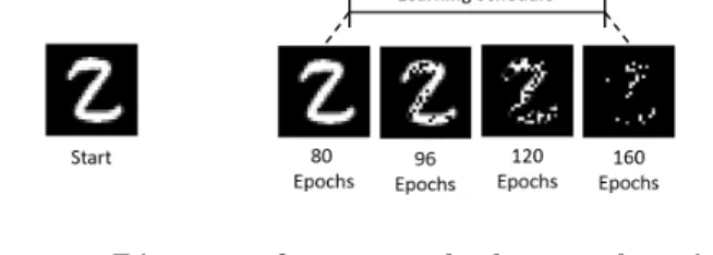
dropout ratepis gradually increased to pf inal. The train-ing schedule of an example input (digit “2”) can be seen
Figure 1: Diagram of an example dropout learning schedule with 160 epochs. The first 80 epochs use zero dropout, but the rate of dropout is gradually increased from 0% to 80% over the last 80 epochs.
in Fig. 1, where the entire digit is presented throughout the first phase, then parts of the image are dropped with a gradually increasing rate in the second phase. While Fig. 1 shows the dropout of the input, all layers of the network similarly have the same dropout level. Three networks for each combination ofpf inal ∈ {0.4,0.5,0.6,0.7,0.8,0.9}and additional training epochse2∈ {20,50,80}were trained.
Since this technique can be performed on an already-trained network, it can be effectively used in combination with ex-isting networks.
2.5.3
Stacked Auto-Encoder with Zero Masking
Similar in motivation to the variants of dropout introduced above, a stacked auto-encoder (SAE) trained with high zero-masking, i.e. replacing input pixels with zero, will learn ef-fective ways to restore a signal even given very little input. Since SAEs are trained with a cost function that measures how well each layer can restore its own input, a high zero-masking rate of e.g. p= 0.9 requires the network to learn to reconstruct the input signal from only 10% of the in-put signal. While the standard approach for ANNs is to use an SAE to extract the signal from corrupt or noisy in-puts, in the domain of SNNs this amounts to generating predictions of the external representation. From the first input spike, the SAE attempts to “undo” the zero-masking caused by the inputs that have not yet arrived. For each additional input spike, the challenge gets easier as the effec-tive zero-masking of time is gradually undone and a more complete signal is provided. SAEs that have been trained with high zero-masking may restore the signal with very lit-tle information, which allows them to begin producing out-puts very quickly. Here we initially train networks as SAE, followed by a discriminative training with classification la-bels foreepochs. Three networks for every combination of zero-masking ratep∈ {0.1,0.3,0.5,0.8,0.85,0.95,0.99}and training epochse∈ {20,50,80}were trained.3.
RESULTS
As described in Sec. 2.3, we evaluate different approaches by quantifying the number of input spikes and the amount of computation necessary to reach 98% accuracy on MNIST. Fig. 2 summarizes the computational cost of running a work trained according to these approaches. Ideally, net-works should be located to the left, which would imply that
Total Computation for >98% Accuracy (Lower is Better) ×106 0.5 1 1.5 2 2.5 3 3.5 4 4.5 SAE (norm.) SAE Sched. (norm.) Sched. Dropout (norm.) Dropout Act. Cost (norm.)
Act. Cost Sparse (norm.) Sparse Default (norm.) Default Frame-based Cutoff
Figure 2: Boxplot indicating amount of computation for SNNs using different optimization approaches. This boxplot indicates minimum, first quartile, me-dian (red line), third quartile, and maximum, with outliers shown as red stars. The majority of the op-timization methods lie to the left of the black ver-tical line, indicating they require less computation than a frame-based ANN to achieve the same 98% classification accuracy. The best result shown here achieves the target accuracy in less than 42% of the computational operations required for an ANN.
98% classification accuracy can be achieved with only a few operations within the network. The black line in Fig. 2 shows the number of operations necessary to arrive at an answer for the frame-based ANN, and nearly all of the ex-amined SNNs require fewer operations. Furthermore, by comparing to the baseline results (labeled “Default,”), we can see that nearly all optimization algorithms offer a sub-stantial improvement. Networks that do not achieve 98% accuracy are not shown; certain parameter configurations such as extremely high dropout or unbalanced cost on the activation prevented these networks from achieving the tar-get accuracy.
It can also be observed that weight normalization decreases computation for most networks. In Fig. 2, normalized net-works from the same optimization algorithm had a tendency to shift the results to the left, implying a decrease of the to-tal amount of computation in the networks. In general, the normalized networks were both faster (lower latency) and more efficient (fewer operations) than their unnormalized counterparts (see Table 1), with the exception of the SAEs. These networks had weights so large that normalization had a tendency to decrease the weights, thus requiring further latency to achieve the same activation.
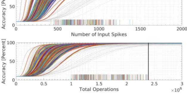
Figure 3 shows the accuracy of all 522 tested networks over time, i.e. either as a function of the number of input spikes (top), or the number of total operations (bottom). Since ev-idence is accumulating over time, these curves are typically monotonically increasing. The thin light gray curves indi-cate networks that did not achieve 98% accuracy within the compute constraint, which is indicated as a black vertical line. For those networks that did achieve 98% accuracy, a colored vertical line on the horizontal axis indicates the point at which the network crossed 98%, and the corresponding
ac-Figure 3: Dependency of accuracy on the number of input spikes and total operations for trained SNNs using different optimization approaches. The top figure depicts the accuracy versus latency while the bottom shows accuracy versus computation. Each line shows the accuracy curve for one of the 522 networks. Curves for networks that achieve 98% accuracy within the compute constraint are plotted in different (but arbitrary) colors, and the remaining networks are plotted in light gray. In both plots, a colored vertical tick mark on the horizontal axis is drawn to indicate the point at which a network passes 98% accuracy. In the bottom figure, the black vertical line indicates the amount of computation required for a frame-based ANN.
curacy curve is plotted in color. One can see that the most efficient networks achieved classification with 0.997 MOps, compared to the fixed computation costs of the frame-based ANN requiring 2.39 MOps. This amounts to a reduction of operations by more than 58%.
Out of all the different networks, the network with the short-est latency to reach 98% accuracy is the SAE, which reaches the desired performance after only 445 input spikes. As mentioned above, the unnormalized SAE networks outper-formed the normalized SAE networks. This is because the weights were so large that they were decreased by the nor-malization process, rather than increased, requiring more spikes to achieve the same level of accuracy. The fastest networks, which are the leftmost curves in Fig. 3, corre-spond to the networks trained with extremely high dropout rates ofp= 0.70 andp= 0.80. However, they were not able to achieve greater than 98% accuracy and so are shown in grey. In fact, even rate-based ANNs before conversion were not able to achieve accuracies above 98.10% with such high dropout rates, so they were excluded from further analysis. In order to compare the influence of different parameter settings for one approach, we plotted a set of performance curves for a given algorithm, in this case the dropout learn-ing schedule (Sec. 2.5.2) in Fig. 4. Highlighted in bright colors are the curves corresponding to all curves for all net-works that use this approach and achieved greater than 98% accuracy in fewer computes than a frame-based ANN. These are 46 of the 54 parameter combinations tested, and the networks have been weight-normalized. Their perfor-mance is tightly aligned, despite the large variations in the
Figure 4: Same as Fig. 3, but highlighting only the results for the 54 SNNs trained with a Dropout Learning Schedule in color, with the remaining SNNs in light gray. One can see the remarkable similarity of learning results for different parameter settings.
Default
Dropout Sparse Coding
Dropout Learn Sched. Activ. Cost
SAE
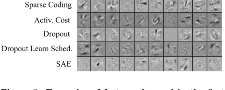
Figure 5: Examples of features learned in the first hidden layer with different optimization approaches. 10 features were selected randomly, and are dis-played with normalized gray levels. Note that, simi-lar to previous studies, Gabor-like and stroke-like features of the MNIST digits appear for all ap-proaches.
tested parameters, indicating robustness to the parameters of the dropout learning schedule. Moreover, these networks achieved the overall lowest compute cost of 0.997 MOps, while simultaneously having among the lowest latency, pro-ducing accurate classification after only 602 input spikes. A summary of the performance results for the different opti-mization methods, together with suggested parameter ranges for each method can be found in Table 1. It shows that in general all methods outperform the default case of an unprocessed SNN by a wide margin. The best methods re-duce computation by 70% of Ops, and the latency by almost 75%. Among the methods tested, we see an advantage for networks trained with dropout learning schedule in the nor-malized case, and SAE in the unnornor-malized case. With the exception of SAE, in general weight-normalization is advan-tageous for all methods.
In order to analyze qualitative differences in the features learned by different learning approaches, each row in Fig. 5 shows ten randomly-selected features (i.e. weight vectors) learned by the first hidden layer connecting to the input
layer. As expected, the first layer learns Gabor-like and stroke-like filters in all cases, thus showing no major differ-ences between the weights learned by different approaches.
4.
DISCUSSION
The purpose of this work is to demonstrate the power and efficiency of spiking neural networks. These networks were able to achieve equivalent classification performance as their rate-based equivalents, and often did so in far fewer opera-tions and with a shorter latency. Due to the efficiency of a spike-based implementation, the input can be correctly clas-sified before a frame-based approach could even read in all the necessary pixels to compute.
Here we examined different methods for incorporating effi-ciency already into the training process of neural networks, thereby allowing networks to learn to be efficient. Overall, nearly all methods and parameter sets yielded much im-proved results in terms of efficiency, while maintaining clas-sification accuracy. Even more encouraging, several different training methods converge to approximately the same fun-damental minima of computation as well as latency (around 1.5 MOps, in Fig. 2), which is a phenomena that warrants further study.
The fastest accurate classification was achieved using unnor-malized SAEs, which reached 98% accuracy after only 420 spikes. A network without any optimization required on av-erage 1753 spikes, which results in a latency more than four times as long. The most efficient network in terms of opera-tions, a normalized network trained with a dropout learning schedule, needs only 1.04 MOps compared to the standard default training of 3.43 MOps, amounting to almost 70% reduction.
While no algorithm clearly wins, and further research can demonstrate how these results extend to other tasks, the newly introduced dropout learning schedule algorithm is per-haps the best to use in practice. It is compatible with ex-isting learned architectures, straightforward to implement, and yields extremely low-compute and low-latency networks. Moreover, when used with existing networks, the overall ac-curacy can be monitored during the learning schedule and training can be terminated early or late, depending on how much accuracy loss is acceptable.
Importantly, the presented SNNs communicate all necessary values with a single binary event, and thus do not rely on a costly multiplier implementation in hardware. Thus, if hardware costs are considered, optimized SNNs might be even more advantageous, since they can be implemented us-ing simple adders, and are thus very amenable to a simple, and low-power optimized hardware implementation.
5.
ACKNOWLEDGMENTS
We acknowledge the EU project SeeBetter (FP7-ICT-270324), Samsung Advanced Institute of Technology, and the Swiss National Science Foundation Grants 200021 146608 and 200021 135066.
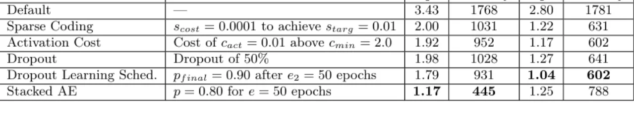
Table 1: Summary of Results: Comparison of the number of operations (measured in millions of adds) and latency (measured as the number of input spikes) necessary to reach 98% accuracy for different optimization approaches. Networks with unnormalized and normalized weights are compared.
Unnormalized Normalized Method Parameters Ops Latency Ops Latency
Default — 3.43 1768 2.80 1781
Sparse Coding scost= 0.0001 to achievestarg= 0.01 2.00 1031 1.22 631
Activation Cost Cost ofcact= 0.01 abovecmin= 2.0 1.92 952 1.17 602
Dropout Dropout of 50% 1.98 1028 1.27 641
Dropout Learning Sched. pf inal= 0.90 aftere2= 50 epochs 1.79 931 1.04 602
Stacked AE p= 0.80 fore= 50 epochs 1.17 445 1.25 788
[1] C. Brandli, L. Muller, and T. Delbruck. Real-time, high-speed video decompression using a frame-and event-based DAVIS sensor. In2014 IEEE
International Symposium on Circuits and Systems (ISCAS), pages 686–689. IEEE, 2014.
[2] Y. Cao, Y. Chen, and D. Khosla. Spiking deep convolutional neural networks for energy-efficient object recognition.International Journal of Computer Vision, pages 1–13, 2014.
[3] P. U. Diehl, D. Neil, J. Binas, M. Cook, S.-C. Liu, and M. Pfeiffer. Fast-classifying, high-accuracy spiking deep networks through weight and threshold balancing. InInternational Joint Conference on Neural Networks (IJCNN), 2015.
[4] C. Farabet et al. Comparison between
frame-constrained fix-pixel-value and frame-free spiking-dynamic-pixel convnets for visual processing.
Frontiers in Neuroscience, 6, 2012.
[5] S. Furber, F. Galluppi, S. Temple, and L. Plana. The SpiNNaker Project.Proceedings of the IEEE, 102(5):652–665, 2014.
[6] A. Hannun et al. Deep Speech: Scaling up end-to-end speech recognition.arXiv preprint arXiv:1412.5567, 2014.
[7] G. Hinton, L. Deng, D. Yu, G. E. Dahl, A.-r. Mohamed, N. Jaitly, A. Senior, V. Vanhoucke, P. Nguyen, T. N. Sainath, et al. Deep neural networks for acoustic modeling in speech recognition: The shared views of four research groups.IEEE Signal Processing Magazine, 29(6):82–97, 2012.
[8] G. E. Hinton et al. Improving neural networks by preventing co-adaptation of feature detectors.arXiv preprint arXiv:1207.0580, 2012.
[9] G. Indiveri, E. Chicca, and R. Douglas. A VLSI array of low-power spiking neurons and bistable synapses with spike-timing dependent plasticity.IEEE Trans on Neural Networks, 17(1):211–221, 2006.
[10] Y. LeCun, Y. Bengio, and G. Hinton. Deep learning.
Nature, 521(7553):436–444, 2015.
[11] Y. LeCun, L. Bottou, Y. Bengio, and P. Haffner. Gradient-based learning applied to document recognition.Proceedings of the IEEE, 86(11):2278–2324, 1998.
[12] S.-C. Liu and T. Delbruck. Neuromorphic sensory systems.Current Opinion in Neurobiology,
20(3):288–295, 2010.
[13] P. Merolla et al. A million spiking-neuron integrated circuit with a scalable communication network and interface.Science, 345(6197):668–673, 2014. [14] V. Mnih, K. Kavukcuoglu, D. Silver, A. A. Rusu,
J. Veness, M. G. Bellemare, A. Graves, M. Riedmiller, A. K. Fidjeland, G. Ostrovski, et al. Human-level control through deep reinforcement learning.Nature, 518(7540):529–533, 2015.
[15] D. Neil and S.-C. Liu. Minitaur, an event-driven FPGA-based spiking network accelerator.IEEE Trans on Very Large Scale Integration (VLSI) Systems, 22(12):2621–2628, 2014.
[16] P. O’Connor, D. Neil, S.-C. Liu, T. Delbruck, and M. Pfeiffer. Real-time classification and sensor fusion with a spiking Deep Belief Network.Frontiers in Neuroscience, 7, 2013.
[17] R. B. Palm. Prediction as a candidate for learning deep hierarchical models of data, 2012.
[18] J. P´erez-Carrasco and others. Mapping from
frame-driven to frame-free event-driven vision systems by low-rate rate coding and coincidence
processing–Application to feedforward ConvNets.
IEEE Trans on Pattern Analysis and Machine Intelligence, 35(11):2706–2719, 2013.
[19] C. Poultney, S. Chopra, Y. L. Cun, et al. Efficient learning of sparse representations with an
energy-based model. InProc. of NIPS, pages 1137–1144, 2006.
[20] K. Simonyan and A. Zisserman. Very deep convolutional networks for large-scale image recognition.arXiv preprint arXiv:1409.1556, 2014. [21] N. Srivastava, G. Hinton, A. Krizhevsky, I. Sutskever,
and R. Salakhutdinov. Dropout: A simple way to prevent neural networks from overfitting.The Journal of Machine Learning Research, 15(1):1929–1958, 2014. [22] E. Stromatias, D. Neil, F. Galluppi, M. Pfeiffer, S.-C.
Liu, and S. Furber. Live demonstration: handwritten digit recognition using spiking Deep Belief Networks on SpiNNaker. In2015 IEEE International
Symposium on Circuits and Systems (ISCAS), pages 1901–1901, 2015.
[23] C. Szegedy, W. Liu, Y. Jia, P. Sermanet, S. Reed, D. Anguelov, D. Erhan, V. Vanhoucke, and
A. Rabinovich. Going deeper with convolutions.arXiv preprint arXiv:1409.4842, 2014.