Secondary Mortgage Market Purchase Yields

Andrea J. Heuson

Finance Department University of Miami Box 248094 Coral Gables, FL 33124-6552 (305) 284-1866 Direct (305) 284-4800 Fax aheuson@miami.edu

Adam Schwartz

Finance Department University of Mississippi University, MS 38677 (662) 915-5729 (662) 915-7960 adam@bus.olemiss.edu

V. Carlos Slawson, Jr.

Finance Department Louisiana State University

2163 CEBA Baton Rouge, LA 70803-6308 (225) 578-6255 Direct (225) 578-6366 Fax cslawson@lsu.edu August 19, 2002

Secondary Mortgage Market Purchase Yields

In this paper we evaluate 15-year and 30-year mortgage origination yields in the secondary mortgage from 1985-2001. We regress house price volatility estimates and readily available term structure parameters on daily, secondary-market, commitment yields provided by FHLMC. We find a strong link between practice and mortgage prepayment and default option theory over time and across market conditions, suggesting that the secondary mortgage market is functioning efficiently. Of note, empirical evidence presented here indicates that volatility in house prices, a standard proxy for the valuation of the option to default, is responsible for a measurable component of required secondary market origination yields.

Secondary Mortgage Market Purchase Yields

A mortgage secured by a home is typically one of the largest financial obligations borne by the individual family unit. Loan origination followed by immediate sale in the secondary market is the dominant method of financing housing in the United States today. Despite the apparent simplicity of the transaction, and the speed with which it can now be accomplished, a mortgage is one of the more complex securities that exists in financial markets. In this paper, we test several hypotheses about the mortgage market. Specifically, we regress house price

volatility estimates and readily term structure variables on a large sample of daily origination data provided by the Federal Home Loan Mortgage Corporation (FHLMC).

To develop our hypotheses, we use a theoretical options pricing mortgage model containing both prepayment and default options to simulate the impact of available parameters on required origination yields. We find that the cross-section and time series behavior of actual commitment yields conforms closely to mortgage theory. This evidence that secondary

mortgage market yields correspond to theory supports the contention that the largest national credit market accessed by individual homeowners is functioning efficiently.

We use secondary market yields of mortgage-backed assets because they possess several features and qualities that make them suitable for our focus. First, these yields incorporate both the loan contract rate and origination fees, standardizing across different combinations offered by lenders. In practice, primary lenders rely heavily on posted purchase yields in setting their offerings to borrowers. Second, the secondary mortgage market is national in scope and is not affected by conditions that might impact primary lenders in certain geographic regions. Third, the secondary market is open to all categories of originators so the yields are not biased by forces unique to thrift, commercial bank or mortgage banking providers of primary market mortgage

credit. Fourth, the secondary market is now the largest provider of mortgage financing—some 60% of mortgage origination volume has been securitized in recent years. Fifth, secondary market yields are not proprietary and a long time series of daily observations derived by securitizers in a consistent fashion is readily available. Our focus on publicly available secondary market yields frees us from the constraint of relying on a privileged data source.

The remainder of this paper is organized as follows. First, we offer a brief review of analytical and empirical mortgage models. Second, we develop testable hypotheses about relationships between readily available parameters and the origination contract rate on

prepayable, defaultable fixed-rate loans, such as those provided by the FHLMC . Third, we then subject these hypotheses to empirical testing for a long time series of actual, daily purchase yields data provided by the FHLMC. Finally, we discuss the extent to which market practice, as evidenced by the empirical determinants of the mortgage-treasury spread, is consistent with theory.

1. Options in Mortgages

1.1 Analytical Models

Initial theoretical research by Dunn and McConnell (1981a, 1981b) values the right to prepay a callable and assumable fixed rate mortgage and simulates secondary market prices of Government National Mortgage Association (GNMA) pass-through securities backed by pools of FHA/VA mortgage loans in a variety of interest rate environments. This work is extended by Archer and Ling (1993), who recognize that the borrower also has the right to default on a loan, and by Kau et al., (1992, 1994), who use a two-state variable specification to incorporate the

competitiveness of the exercise of mortgage options.1 Hilliard et al. (1998), the analytical model used in this paper, provides a binomial alternative to the finite-difference techniques used by Kau et al. (1992, 1994) and greatly improve computational efficiency when compared to

non-recombining bivariate binomial trees.

Further enhancements have been added to analytical models to focus on specific

complexities the administrative structure of the primary mortgage market adds to the valuation of loans containing two embedded interacting options. For example, primary lenders may offer two or more combinations of loan contract rate and origination points to individual borrowers and combinations differ across lenders on any given day, despite the fact that a secondary market purchaser sets a single price each day for a conforming loan of a given maturity. LeRoy (1996) analyzes the contract rate/points tradeoff at the loan level as a semi-pooling equilibrium where origination fees separate borrowers based on unobservable prepayment probabilities. Stanton (1995) models the idiosyncratic prepayment behavior of a mortgage pool by assuming that refinancers face heterogeneous transactions costs while Stanton and Wallace (1995) allow characteristics of the replacement mortgage to impact the decision to prepay an existing loan. All of these models concur in finding that increases in the probability of prepayment raise the yield a lender requires to originate a loan—a result that receives strong empirical support in this paper.

Dunn and Spatt (1999) use arbitrage methods to investigate the interaction between maturity, amortization and points in valuing default-free callable debt contracts. They

demonstrate that the amortization feature implies that a loan’s contract rate and the value of its

1_{FHA/VA loans, which were the focus of Dunn and McConnell’s research, are freely assumable.} Since the early 1980s, conventional loans, (the type usually traded in the secondary mortgage market), have not been assumable. As a result, later models do not allow a borrower to transfer a mortgage if the ownership of the home changes during the loan’s life.

embedded prepayment option rise with maturity. This result, which is consistent with traditional option valuation theory, holds despite the fact that the Dunn and Spatt approach does not rely on assumptions about the shape of the term structure, the stochastic process of interest rates,

borrower preferences or idiosyncracies of the mortgage market. Our empirical evidence supports the analytical work of Dunn and Spatt in that the required yield on a mortgage is a positive function of a loan’s maturity across a variety of financial market conditions.

Ambrose, Buttimer and Capone (1997) focus on the option to default. They incorporate institutional delays in the foreclosure process which allow the borrower to live in the home without paying rent. These delays trade off against the transaction costs of foreclosure and the possibility of deficiency judgements against delinquent homeowners. Simulation results suggest that an unwillingness to pursue deficiency judgements has led to substantially higher default rates on FHA and VA loans. Empirical evidence presented here indicates that volatility in house prices, a standard proxy for the value of the option to default, is responsible for a measurable component of required secondary market origination yields.

1.2 Empirical Tests

Many authors use valuation models to simulate the prices of mortgages with embedded options or to predict expected prepayment behavior. Schwartz and Torous (1989) integrate a prepayment function estimated from actual loan terminations into the Brennan and Schwartz (1982, 1985) two-factor interest rate model for default free securities. Their simulations conform to the observed behavior of generic mortgage-backed security prices during the precipitous mid-1980s decline in interest rates. Stanton (1995) uses his heterogeneous transaction costs model to simulate prepayment rates on mortgage-backed securities and finds that the resulting termination

functions forecast actual refinancing flows at least as well as those of the Schwartz and Torous model. These papers do not compare simulated and actual mortgage values, however,

presumably because trade prices on mortgage-backed securities are proprietary data. Our focus on publicly available secondary market yields frees us from the constraint of relying on a privileged data source.

Collin-Dufresne and Harding (1999) derive a closed-form solution for a one-state variable model (the short term interest rate) with an embedded prepayment expectation function and compare the prices generated to monthly average mortgage-backed security values from the early 1990s. Although the closed form approach is faster than a binomial tree, and the resulting estimated prices fit the data reasonably well, the analytical results cited in the previous section of this paper show that the house price process (which controls the value of the option to default) is an integral component of the value of a standard mortgage.

Chatterjee, Edmister and Hatfield (1998) collect actual loan originations from a multi-state primary lender during the 1990s and use the initial value of these mortgages to discriminate between various multi-state mortgage valuation models on the basis of predictive accuracy. They find that a two-factor model incorporating house value and a spot interest rate is more efficient than a two-factor interest rate model, (which incorporates a long-term yield and a spot rate), with or without an additional house price component. This result leads us to select the Kau, et al. (1992, 1994) framework and the bivariate binomial model specification of Hilliard, et al. (1998) as our source for predictions about the expected behavior of mortgage origination yields.

Related empirical work focuses on comparing market yields on mortgages to those on securities that lack embedded options. Early research (e.g. Black, Garbade and Silber (1981),

Hendershott, Shilling and Villani (1983) and Hall (1985)) establishes the spread between a mortgage yield and a Treasury yield for a maturity equal to the expected life of the mortgage as a proxy for the option premium demanded to originate a pre-payable loan. Extensions such as Nothaft, Rothberg and Gabriel (1989) and Kolari, Frazier and Anari (1998) demonstrate that this spread changes with market conditions in a manner consistent with standard option pricing theory. For example, the MBS-Treasury spread (M-T spread) increases in volatile markets and when the term structure flattens (the downward sloping yield curve is thought to signal lower market rates, which could spur prepayments). Archer and Ling (1997), among others, note that principal protection on loans sold in the secondary market means that mortgage default generates the early return of principal for the investor. Therefore, changes in default and prepayment option values have the same impact on the M-T spread.

Bradley, Gabriel and Wohar (1995) analyze monthly values of the M-T spread to determine the impact of changes in the amount of mortgage credit supplied by savings and loan institutions on the cost of mortgage funds. They find that a significant structural shift occurred in the residential mortgage market beginning in mid-1982. This shift is attributed to technical and regulatory changes that allowed the separation of the mortgage origination, servicing and portfolio functions. These developments increased competition and operational efficiency in the market to the point where it may no longer have been profitable for thrift originators to hold mortgage loans. Statistical tests show that increases or decreases in the amount of mortgage credit supplied by thrift institutions did not have an impact on the M-T spread in the later portion of the sample, ostensibly because of the dominance of securitization. Our empirical analysis is performed on a sample of secondary market origination yields that begins in 1985 in order to

insure that all the data we are evaluating is drawn from a market where the characteristics of the mortgage, not the originator, governs the pricing of the loan.

Despite the importance of securitization to the mortgage origination industry and the improvements in computational power and theoretical sophistication in mortgage modeling, to our knowledge, no one has evaluated the actual behavior of origination yields in a secondary market to determine whether practice conforms to theory over time and across market conditions.

2. Testable Hypotheses for Specific Environments

We next develop hypotheses about the behavior of secondary mortgage market

origination yields during the 1980s and 1990s by reviewing and using existing mortgage theory to simulate option values and equilibrium contracted rates in specific environments.

2.1 The Valuation Model

The value of a mortgage loan M is a function of the spot rate r, the house value H, the contract rate c, the mortgage maturity m, and the loan-to-value ratio l, so that:

M = PVRP – C – P (1)

where,

PVRP = the present value of the remaining mortgage payments C = the value of the prepayment option (a call), and

P = the value of the default option (a put).

We use the two-variable binomial technique of Hilliard et al. (1998) to incorporate the prepayment option and the default option via the following risk neutral processes:

(3) , ) ( (2) and , ) ( ^ ^ r r H H dz r dt r dr dz dt s r H H d

σ

κ

σ

+ − Π = + − = where,

H = the house price,

s = the service flow from the house,

κ

= the speed of adjustment to the long-term mean,

Π = the long-term mean interest rate,

H

σ

= the volatility of the house price process,

r

σ

= the volatility of the interest-rate process, and

r H dz

dz , are Wiener processes with correlation

φ

.

To ensure a computationally simple bivariate binomial lattice, the processes (2) and (3) are transformed as demonstrated in Nelson and Ramaswamy (1990) and applied in Hilliard, Schwartz and Tucker (1996) to achieve unit-volatility. The transformed differentials are then transformed again to insure constant variances and achieve independence. The resulting stochastic diffusions are uncorrelated and can be modeled on a recombining lattice.

2.2 Simulated Prepayment and Default Option Values and Option Adjusted Loan Contract Rates

Our simulations mimic actual origination practices. Residential loans are quoted in combinations of contract rate and origination points and then sold in the secondary market on the basis of the yield implied by these two parameters and a standard loan life, (typically 5 to 7 years for a 15-year loan and 10 to 12 years for a 30-year loan). Borrowers choose loan amounts

subject to payment-to-income and loan-to-appraised value constraints2. We assume origination fees of 1.5%, (a typical value) and solve simultaneously for the contract rate and corresponding default and prepayment option values for loans that would be priced at 98.5% of par. This strategy produces the minimum contract rate needed to induce a lender to make a loan with a pre-determined loan-to-value ratio and maturity, given the current spot rate3.

Changing financial market conditions affect the expected interest rate parameters of the valuation model,

κ

and

σ

_r, and the volatility of the house price process,

σ

_H. Our simulations study the impact of representative assumptions for each of these inputs and initial mortgage maturity on prepayment and default option values and the corresponding option adjusted contract rate a lender requires to originate a loan. We vary the current spot rate (r), the speed of

adjustment (κ), and the interest rate and house price volatilities (σr and σH) while holding the

base parameters of the governing diffusions constant at: s = annualized service flow = 8.5%,

Π = long-term mean of the spot interest rate = 7.5%, and

φ

= correlation between the house price process and the interest rate process of 0%4.

Each panel of Table 1 shows the individual components of the mortgage value, PVRP, C

and P, (the present value of the remaining payments, the call option to prepay and the put option

2_{Loan payments inclusive of escrows are typically constrained at less than 25% to 28% of gross} consistent income while total long-term debt payments can consume no more than 33% to 36% of that income.

3_{The mortgage valuation model assumes the Cox, Ingersoll and Ross (1979) interest rate}

process, which is neutral in terms of interest rate risk. Any interest rate risk premium is absorbed by Π and

κ

(Eq. 3), so the instantaneous spot rate is only additional parameter needed to

complete the interest rate specification.

4_{Thesimulations do not include transactions costs faced by borrowers who prepay or default.} Kau and Slawson (2002) demonstrate how these frictions can be incorporated into the bivariate binomial model used in this paper.

to default, respectively) as a percentage of the par value of the loan, (lH0). The actual mortgage value, which is constrained to be 98.5% of par, is the net of the component parts.

The first three panels of Table 1 display outcomes for changing house price and interest rate volatility under three interest rate environments that mimic conditions in the mortgage market over the past fifteen years. Given that securitization practice assumes a standard life of 5 to 7 years for 15-year loans and 10 to 12 years for 30-year loans, we choose the 10-year constant maturity Treasury yield as a market proxy for the spot rate. The 10-year yield has been quoted on a daily basis since January 1962. Its value averaged 7.46% over the January, 1962 –

September, 2001 time period, with a high of 15.84% and a low of 3.78%. The mean 10-year constant maturity yield was 7.65% from January, 1962 to December, 1984, (prior to the beginning of our sample) and 7.19% from January, 1985 to September, 2001, (our sample period). Therefore, we chose 7.5% as the long term mean. In addition, the simulations in the first three panels assume a speed of reversion to the long-term mean of 25% while 15% and 5% are chosen to measure high and low house price and interest rate volatility levels, respectively.

Panel 1 of Table 1 assumes current interest rates 300 basis points above the assumed long-term mean of 7.5%, (a spot rate of 10.5% and a downward-sloping term structure) as in the 1980s. Results for interest rates 150 basis points below the long-term mean, (a spot rate of 6%, which leads to a mildly upward-sloping term structure), corresponding to the refinancing boom of the early 1990s, appear in Panel 2. Panel 3 reflects the historically low level of interest rates in the late 1990s, (here the spot rate is 3% and the term structure slopes upward steeply).

The top three panels of the Table underscore the importance of interaction effects between put and call option values as other conditions change. Comparing the left-most (both volatilties high) and right-most (both volatilities low) 30-year or 15-year simulations (Columns

(1) and (4) holding maturity constant) for each level of the spot rate shows how dramatic an effect changing volatilities can have on option values and option-adjusted contract rates. As long as one of the two volatilities is at the “high” level, one of the two option values is at least 4% of the par value of the mortgage. Furthermore, simulated prepayment option values are close to half of the par value of a 30-year mortgage while default option values can measure 20% of the face value of a long-term loan using base parameters representative of actual market data.

Reading down any column of the first three panels of the table provides further evidence of the complex relationship between the present value of the loan payments and the default and prepayment option values. In general, the decline in the value of the call option as the spot rate falls is somewhat offset by an increase in the value of the default option. Therefore, the present value of the expected payments generated by the contract rate over the life of the loan and the option-adjusted contract rate drop along with the spot rate but at a slower rate of descent.

The contract rate to spot rate spreads in Table 1 are a convenient way to capture the multiple components of the value of a fixed-rate mortgage with embedded options. They allow us to compare theoretical predictions directly to the actual evolution of origination rates on loans sold in the secondary mortgage market. These yields that make up the spreads are observable on a daily basis over a long sample period that covers a wide variety of term structure slope, interest rate volatility and reversion, and house price volatility conditions.

2.3 Testable Hypotheses

Study of the first three panels of the table generates the following six testable hypotheses: 1) Reading down any column, the spread is positively related to the slope of the term structure, (defined as the 7.5% long term mean of the interest rate process less the current spot rate), within each maturity for all volatility combinations.

2) Reading down any column, the rate of increase in the contract rate to spot rate spread rises as the slope of the term structure rises, (the spot rate falls).

3) Within any of the 4 columns, the option-adjusted contract rate to spot rate spread is larger for a 30-year loan than a 15-year loan, ceteris paribus.

4) Reading down any column and comparing across maturity sub-columns, the spread widens faster for longer term loans as term structure slope increases, (the spot rate falls).

5) Comparing Column 1 to Column 2 and Column 3 to Column 4 within any panel, the spread increases with house price volatility for a given maturity.

6) Comparing Column 1 to Column 3 and Column 2 to Column 4 within any panel, the spread increases with spot rate volatility for a given maturity.

Panel 4 addresses the impact of different assumptions regarding the speed of reversion. All of the assumed parameter values are representative of actual market conditions during the period covered by the sample data5. The fourth panel of the table demonstrates the importance of the assumption of mean reversion in the interest rate process to the valuation of a fixed rate mortgage with embedded options. A higher speed of reversion serves to decrease the expected life of a high-coupon mortgage, (the downward sloping term structure section in the left-hand

5_{Estimation procedures used to actually estimate expected volatility and reversion parameters are} discussed in the empirical section of the paper.

side of the table), with a corresponding decrease in prepayment option value and contract rate to spot rate spread. In contrast, faster reversion to a higher spot rate requires a larger present value of the expected payments when the term structure slopes upward. In this instance, the contract rate to spot rate spread increases with the speed of reversion. Panel 4 of Table 1 yields an additional testable hypothesis regarding the impact of changing the speed of reversion of the interest rate process to its long-term mean:

7) The impact of the speed of reversion on the contract rate to spot rate spread is a function of the slope of the term structure, with a negative relationship expected for downward sloping term structures and a positive relationship expected for upward sloping yield curves.

3. Empirical Tests of Purchase Yield Hypotheses

3.1 The Mortgage Contract Rate Data

We employ a long time series of daily data on secondary mortgage market commitment rates for 15-year and 30-year mortgages purchased by the Federal Home Loan Mortgage Corporation to determine whether or not option-adjusted contract rate to spot rate spreads conform to the predictions of the bivariate binomial option pricing model. The contract rates reflect the return required by Freddie-Mac to purchase loans within the next 30 days and are stated net of the fee retained by the loan servicer. The data set runs from March 15, 1985 to August 15, 2001, (beginning after the structural shift in the mortgage market identified by Bradley, Gabriel and Wohar (1995)) and contains more than 8,200 observations, (more than 4,100 per maturity). It covers a broad spectrum of general financial and mortgage market

conditions such as the relatively high interest rate period of the mid-1980s, the refinancing boom of the late-1980s and the sustained period of low mortgage rates observed in recent years.

3.2 The Empirical Specification

We hypothesize the following empirical relationship for the combined time series of 15-year and 30-year mortgage origination yield spreads over the three-month T-Bill yields, (our proxy for the current spot rate):

SPRm,t = α0 + β1(SLOPE) + β2(SPOT RATE2) + β3(DUM30) +

β4 (SPOT RATE*DUM30) + β5(HOUSEVOL) + β6 (YIELDVOL) +

β7 (REVERSION) + β8 – 18 (MONTHt) + εm,t (8)

where:

SPRm,t = the spread between the 30-year or 15-year secondary market mortgage rate

and the secondary market three-month T-Bill yield for each day in the sample, combined so that there are two observations for each day, SLOPE = the current slope of the term structure (ten-year constant maturity yield -

three-month Treasury Bill yield),

SPOT RATE = the current value of the three-month T-Bill yield,

DUM30 = a binary variable that is one for observations on the 30-year loan spread,

YIELDVOL = the expected volatility of the underlying interest rate process, HOUSEVOL = the expected volatility of the underlying house price process,

REVERSION = the absolute value of the expected speed of reversion of the interest rate process to its long-term mean multiplied by the current slope of the term structure,

MONTHt = a binary variable that takes on the value of one for daily observations in a

given month6 , and

εm,t = an error term that has desirable statistical properties given potential auto-

correlation and heteroscedasticity.

If the prediction of Hypothesis 1 in Table 1 holds, the option-adjusted contract rate-to-spot rate spread, which combines the positive effect of the present value of the expected loan payments and the negative impact of the dual option values, will rise as the term structure of interest rates rises, (short-term rates fall). Thus, we expect (β1 > 0). The squared spot yield term

is included to capture non-linearities in the relationship between this spread and the yield curve slope. Given that the predicted distance widens more rapidly as the spot rate drops, (Hypothesis 2), the coefficient on β2 should be negative.

The coefficient of DUM30 will be positive (β3> 0) if increased option values require that

the spread on a 30-year loan exceed that on a 15-year loan in all market conditions, as in Hypothesis 3. It follows that the positive relationship between loan maturity and option value requires the coefficient on the interaction term (SLOPE * DUM30), to be negative (β4 < 0) so that

the option-adjusted 30-year spread exceeds the 15-year spread by a larger amount at steeper term structure slopes, (lower spot rate levels), as in Hypothesis 4.

If the spread rises with house price and interest rate volatility, two variables that measure the negative impact of options held by the borrower, then (β5 >0) and (β6 > 0), as stated in

Hypotheses 5 and 6, respectively. In addition, if the contract rate to spot rate spread drops with faster reversion to the long term mean with downward sloping term structures but rises with faster reversion for upward sloping yield curves, (Hypothesis 7), then the estimated coefficient

for β7 will be positive. Finally, as noted in Schwartz and Torous (1989), more home sales occur

in the summer months. In order to account for this seasonality, we include monthly binary variables to measure the impact of changes in securitization volume on mortgage rate-to-spot rate spreads.

3.3 Estimates of Expected Interest Rate and House Price Volatility and the Speed of Reversion

Given the obvious difficulties in applying traditional linear regression formulae to long series of daily interest rate data, and the potential asymmetry in error term distributions for 15-year and 30-15-year loans, we will apply a GARCH (1,1) estimation routine containing an AR (4) auto-regressive specification to determine the coefficients of Equation (8)7. Following Bennett, Peach and Peristiani (2000), we also employ the GARCH methodology to estimate expected house price and yield volatilities.

Expected interest rate volatility values are based on monthly yield fluctuation forecasts generated using the Cox, Ingersoll and Ross (1979) short-rate process as described by Chan, Karolyi, Longstaff and Sanders (1992). The expected volatility regressions take the general form:

rt – rt-1 = α + βrt-1 + εt (9)

where:

7 _{The GARCH specification takes the following form:} εm,t = hm,t1/2 (ët)

hm,t = ARCH0 + ARCH1 (εm,t-1) + GARCH1 (hm,t-1) , and

ë ~ Independent, Normal (0,1)

Here, ARCH0 measures the level of the variance process while ARCH1 and GARCH1 measure

the impact of the recent and historical squared residuals, respectively. The sum of the ARCH1

rt = the monthly average value of daily average three-month T-Bill yields,

E[εt] = 0, and

E[εt2] = σ2 rt-1

Each month Equation (9) is estimated over the past two years of monthly averages of daily changes in the secondary market yield of the 90-day Treasury Bill under a GARCH (1,1) specification. The volatility parameter σ2 _{is part of the standard output in the Version 8 SAS}

HETERO sub-routine and the speed with which the spot rate is currently reverting to its long term mean is the beta coefficient in each rolling regression of Equation (9). By construction, the beta coefficient is less than zero if mean reversion is present in the interest rate data and larger negative values indicate an increasing speed of reversion. We use the absolute value of each month’s estimate when fitting the regressions of Equation (8) to simplify the interpretation of the results.

Forecasts for expected house price uncertainty are computed in a similar fashion, but for each quarter, using annualized percentage changes in the Office of Federal Housing Enterprise Oversight’s repeat sales house price index. Here we estimate over the current quarter and the previous nineteen quarters and include quarterly binary variables to allow for seasonality in the underlying data8

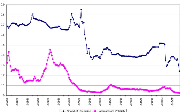
Monthly values for expected interest rate variability and speed of reversion are displayed in Figure 1 and appear reasonable. Spot rate volatility typically varies between 20% and 40% in the late 1980s and early 1990s before settling down to an average of 5% to 10% for the duration of the sample. Speed of reversion values average 70% in the first half of the sample and 40% in the later portion.

Quarterly proxies for expected house price volatility and the underlying housing

appreciation rate appear in Figure 2. House price volatility averages 15% in the early part of the sample period and 10% in recent months but the rate of increase in housing prices has been less predictable in recent years. Taken together, the estimated values in Figures 1 and 2 reassure us that the base parameter assumptions that govern the simulations used to construct Table 1 are representative of market conditions during the sample period.

3.4 Estimation Results

The expected volatility and reversion estimates shown in Figures 1 and 2 and daily values for the slope of the term structure and the current spot rate provide the independent variables for the empirical specification of Equation 8. Estimation results for the entire sample and sub-periods that divide the 15+ year period into three approximately equal segments appear in Table 2. Most of the independent variables are highly significant in the expected direction in the full sample and sub-period regressions. In addition, the overall explanatory power of the equation is consistently high, providing further support for the option valuation model’s predictions.

Specifically, the option-adjusted contract rate to spot rate spread widens as the slope of the term structure increases, (the spot rate falls relative to its long-term mean). As noted in Hypothesis 1, (which predicted a positive coefficient for β1), this result occurs because

increasing default option values mitigate some of the decline in prepayment option values and thus prevent the option-adjusted contract rate from dropping as fast as the spot rate. Simulation results in Table 1 show that the net effect of the negative impact of put and call option values increases as the spot rate falls. This result is corroborated by the negative estimated coefficient for β2, the squared spot yield term addressed in Hypothesis 2. The negative coefficient allows

the spread to widen further at lower spot rates, incorporating the non-linearity in the relationship between the option-adjusted contract rate and the spot rate spread within any single column of Table 1.

The option-value component of this relationship is always larger for a 30-year loan than for a 15-year loan because both prepayment and call option values are positively related to a loan’s maturity. Hence, the contract rate to spot rate spread is always larger for 30-year loans and it widens faster for longer-term loans as the spot rate falls. The positive coefficient for DUM30 predicted by Hypothesis 3 and the negative coefficient for the (SPOT YIELD*DUM30)

interaction term predicted by Hypothesis 4 capture these effects. Their empirical support in Table 2 strengthens the correlation between the analytical results of Table 1 and the actual behavior of mortgage origination yields as the level of spot rates rises and falls across the sample period still further.

It is interesting to note that the interaction term is insignificant in the most recent five-year segment of the sample. This time period reflects historically low spot yields and relatively low volatility in interest rates and house prices, all market conditions which tend to minimize both prepayment and call option values. This may explain why there is no statistical difference between the behavior of 30-year origination rates and 15-year origination rates in the right-most column of Table 2.

Consistent with option pricing theory, the contract rate to spot rate spread rises with increases in the proxies for expected volatility in both housing prices and interest rates. The positive coefficients for HOUSEVOL and YIELDVOL corroborate Hypotheses 5 and 6,

respectively. In the segmented samples, the HOUSEVOL coefficient is largest during the 1985-1989 time period and the YIELDVOL coefficient is largest during the 1990-1994 interval.

Figure 2 shows that expected house price volatility dropped dramatically after 1990 so the regression results may be documenting a shift in emphasis from default options to prepayment options in the secondary mortgage market at that time. A steady decline in market yields and a steady increase in refinancing volume both began in the early 1990’s so the estimated

coefficients are consistent with both market experience and option pricing theory.

The simulation results in the fourth panel of Table 1 predict that the contract rate to spot rate spread will fall dramatically with faster mean reversion when the spot rates temporarily exceed the long-term mean but rise gradually with faster mean reversion when spot rates are temporarily low. Therefore, we constructed the REVERSION variable, (β7, discussed under

Hypothesis 7), by multiplying the absolute value of the expected speed of reversion by the slope of the term structure and expected the estimated coefficient to carry a positive sign9. This result does occur over the full sample and most of the sub-samples but REVERSION coefficients are not significantly different from zero. Further inspection of the values for the empirical proxies for YIELDVOL and the speed of reversion displayed in Figure 1 show that the two series exhibit similar patterns over the entire sample period. This suggests that the value of adding the

REVERSION variable to a specification that already contains YIELDVOL is marginal at best. The coefficients of all of the error correction variables are significant in all regressions, underscoring the importance of allowing for changes in the overall financial environment across the long sample period. Autoregressive parameters are generally significant. Specifically, first through fourth order coefficients are significant in the full sample while first and second order and either third or fourth order coefficients are significant in the sub-samples.

9_{We take the absolute value of the speed of reversion coefficient estimated each month because} those values are negative by construction.

Coefficients on dichotomous variables that measure the impact of seasonality caused by calendar-based changes in securitization volume are consistently negative when significant in January, February and March. In addition, they are positive when significant in September and October. The size of the coefficients is less than 3 basis points in absolute value when

significant in either direction. This shows that origination yields in the secondary mortgage market are positively related to origination volume but that the size of the effect is quite small.

4. Summary and Conclusions

We examine a 15-year time series of daily data secondary mortgage market commitment rates to determine whether observed pricing behavior in the secondary mortgage market is consistent with the predictions of mortgage option pricing theory. We use an analytical

mortgage valuation model to develop hypotheses for the behavior of the equilibrium contract rate under market conditions representative of the three time periods, 1985-1989, 1990-1994, and 1995-2001. This methodology captures the myriad influences on the value of a prepayable, defaultable fixed-rate loan in an empirically tractable form.

As shown in this paper using ranges of parameters consistent with market experience, mortgage theory predicts that:

1) the spread between the option-adjusted mortgage contract rate and the current spot rate increases at an increasing rate as the slope of the term structure rises, (the spot rate falls relative to its long-term mean),

2) the spread increases at a faster rate as spot yields fall, 3) the spread is always greater for longer term loans,

4) 30-year premia exceed 15-year premia by a greater amount in low spot rate environments,

5) increased house price volatility increases the option adjusted contract rates and spreads,

6) increased interest rate volatility increases the option adjusted contract rates and spreads, and

7) the relationship between the option adjusted contract rate spread and the speed of reversion to the long-term mean in the interest rate process depends upon the slope of the term structure.

The 15-year sample of daily, secondary-market, commitment data provided by the

Federal Home Loan Mortgage Corporation for our empirical tests demonstrates that the behavior of the origination rates on 15-year and 30-year loans is very consistent with the predictions of the option model. Hypotheses 1 through 6 are supported empirically, providing strong evidence that mortgage yields are set efficiently under a variety of market conditions. The coefficient for our reversion measure in Hypothesis 7 is not statistically different from zero in the full sample or in any of the subperiods. Given the size of the secondary market for fixed-rate residential

mortgages and the weight attached to the mortgage liability in the portfolios of individual homeowners, efficient pricing of loans over time and in cross-section is an important result from a both a theoretical and a social welfare perspective.

References

Ambrose, B., R. Buttimer and C. A. Capone. “Pricing Mortgage Default and Foreclosure Delay.”

Journal of Money, Credit and Banking 29 (1997), 314-325.

Archer, W.R., and D. C. Ling. “Demographic vs. Option Drive Mortgage Terminations.” Journal of Housing Economics 6 (1997), 137-163.

_______ “Pricing Mortgage-Backed Securities: Integrating Optimal Call and Empirical Models of Prepayment.” AREUEA Journal 21 (1993), 373-404.

Bennett, P., R. Peach and S. Peristiani. “Implied Mortgage Refinancing Thresholds.” Real Estate Economics 28 (2000), 405-434.

Black, D. G., K.D. Garbade and W. L. Silber. “The Impact of the GNMA Pass-Through Program on FHA Mortgage Costs.” Journal of Finance 36 (1981), 457-469.

Bradley, M.G., S.A. Gabriel and M.E. Wohar. “The Thrift Crisis, Mortgage-Credit

Intermediation, and Housing Activity.” Journal of Money, Credit and Banking 27 (1995), 476-497.

Brennan, M. J. and E. S. Schwartz. “An Equilibrium Model of Bond Pricing and a Test of Market Efficiency.” Journal of Financial and Quantitative Analysis 17 (1982), 201-229. _______ “Determinants of GNMA Mortgage Prices.” AREUEA Journal 13 (1985), 209-228. Chan, K. C., A. Karolyi, F.A. Longstaff and T. Sanders, “An Empirical Comparison of

Alternative Models of the Short-Term Interest Rate.” Journal of Finance 47 (1992), 1209-227.

Chatterjee, A., R. O. Edmister and G. B. Hatfield. “An Empirical Investigation of Alternative Contingent Claims Models for Pricing Residential Mortgages.” Journal of Real Estate Finance and Economics 17 (1998), 139-162.

Collin-Dufresne, P. and J. P. Harding. “A Closed Form Formula for Valuing Mortgages.”

Journal of Real Estate Finance and Economics 19 (1999), 133-146.

Cox, J.C, J.E. Ingersoll and S. Ross. “Duration and the Measurement of Basis Risk.” Journal of Business 52 (1979), 51-61.

Dunn, K. B and J. J. McConnell. “Valuation of GNMA Mortgage-Backed Securities.” Journal of Finance 36 (1981a), 599-616.

_________ “Rate of Return Indexes for GNMA Securities.” Journal of Portfolio Management 7 (1981b) 65-74.

Dunn, K.B. and C. S. Spatt. “Call Options, Points and Dominance Restrictions on Debt Contracts.” The Journal of Finance 54 (1999), 2317-2337.

Hall, A.R. “Valuing the Mortgage Borrower’s Prepayment Option.” AREUEA Journal 13 (1985), 229-247.

Hendershott, P.H., J.D Shilling. and K.E. Villani. “Measurement of the Spread Between Yields on Various Mortgage Contracts and Treasury Securities.” AREUEA Journal 11 (1983), 476-490.

Hilliard, J.E., J.B. Kau and V.C. Slawson, Jr. “Valuing Prepayment and Default in a Fixed Rate Mortgage: A Bivariate Binomial Options Pricing Technique.” Real Estate Economics 28 (1998), 431-468.

Hilliard, J.E., A. L. Schwartz and A. L. Tucker. “Bivariate Binomial Options Pricing (With an Application to American Futures Options with Stochastic Interest Rates).” Journal of Financial Research 19 (1996), 585-602.

Kau, J.B., D.C. Keenan, W.J. Muller III and J. Epperson. “A Generalized Valuation Model for Fixed-Rate Residential Mortgages.” Journal of Money, Credit and Banking 24 (1992), 279-299.

_______ “The Value at Origination of Fixed Rate Mortgages with Default and Prepayment Options.” Journal of Real Estate Finance and Economics 11 (1992), 5-36.

Kau, J.B.and V.C. Slawson, Jr. “Frictions, Heterogeneity, and Optimality in Mortgage Modeling.” Journal of Real Estate Finance and Economics 24:3 (2002), 239 – 260. Kolari, J.W., D. R. Fraser and A. Anari. “ The Effect of Securitization on Mortgage Market

Yields: A Cointegration Analysis.” Real Estate Economics 26 (1998), 677-693. LeRoy, S. “Mortgage Valuation Under Optimal Prepayment.” Review of Financial Studies 9

(1996), 677-707.

Nelson, D. and K. Ramaswamy. “Simple Binomial Processes as Diffusion Approximations in Financial Models.” Review of Financial Studies 3 (1990), 393-430.

Nothaft, F. E., J.P. Rothberg and S.A. Gabriel. “On the Determinants of Yield Spreads Between Mortgage Pass-Throughs and Treasury Securities.” Journal of Real Estate Finance and Economics 2 (1989), 301-325.

Schwartz, E. S. and W. N. Torous. “Prepayment and the Valuation of Mortgage-Backed Securities.” The Journal of Finance 44 (1989) 375-392.

Stanton, R. “Rational Prepayment and the Valuation of Mortgage-Backed Securities.” Review of Financial Studies 8 (1995), 677-708.

Stanton, R. and N. Wallace. “Mortgage Choice: Whats the Point?” Working Paper, University of California at Berkeley 1995.

_____________________________________________________________________________________

TABLE 1: Option Values, Option Adjusted Contract Rates and Contract Rate to Spot Rate Spreads for 90% Loan-to-Value 15- and 30-year Mortgages Under Different Initial Term Structure, Interest Rate Volatility and Speed of Reversion Assumptionsa

______________________________________________________________________________ Panel 1: Current Spot Rate = 10.5% (Term Structure Slope = -3.0%, Downward Sloping)a

(1) (2) (3) (4)

σr = 15%, σH = 15% σr = 15%, σH = 5% σr = 5%, σH = 15% σr = 5%, σH = 5%

30-Year 15-Year 30-Year 15-Year 30-Year 15-Year 30-Year 15-Year

PVRP 162.06% 131.16% 144.87% 122.64% 135.13% 115.18% 114.96% 106.10%

Call 49.07% 25.48% 46.03% 24.08% 24.15% 11.07% 16.08% 7.57% Put 14.49% 7.18% 0.34% 0.05% 12.48% 5.61% 0.39% 0.03%

Option-adjusted Mortgage Contract Rate

13.74% 13.31% 12.15% 12.03% 12.06% 11.43% 10.02% 9.97% Contract Rate to Spot Rate Spread

3.24% 2.81% 1.65% 1.53% 1.56% 0.93% -0.48% -0.53%

Panel 2: Current Spot Rate = 6.0% (Term Structure Slope = 1.5%, Mildly Upward Sloping)a

(1) (2) (3) (4)

σr = 15%, σH = 15% σr = 15%, σH = 5% σr = 5%, σH = 15% σr = 5%, σH = 5%

30-Year 15-Year 30-Year 15-Year 30-Year 15-Year 30-Year 15-Year

PVRP 146.60% 121.74% 123.47% 111.16% 127.03% 109.87% 103.39% 100.02%

Call 30.82% 15.75% 22.47% 12.42% 14.59% 5.49% 2.86% 1.42% Put 17.28% 7.49% 2.50% 0.24% 13.94% 5.89% 2.03% 0.10%

Option-adjusted Mortgage Contract Rate

10.70% 9.86% 8.70% 8.31% 9.63% 8.51% 7.39% 6.97% Contract Rate to Spot Rate Spread

_________________________________________________________________________________ Panel 3: Current Spot Rate = 3.0% (Term Structure Slope = 4.5%, Steeply Upward Sloping)a

(1) (2) (3) (4)

σr = 15%, σH = 15% σr = 15%, σH = 5% σr = 5%, σH = 15% σr = 5%, σH = 5%

30-Year 15-Year 30-Year 15-Year 30-Year 15-Year 30-Year 15-Year

PVRP 138.08% 115.90% 113.61% 103.85% 122.88% 107.21% 102.15% 98.77%

Call 20.11% 9.52% 8.21% 4.89% 9.32% 2.68% 0.24% 0.10% Put 19.46% 7.88% 6.91% 0.46% 15.06% 6.04% 3.41% 0.17%

Option-adjusted Mortgage Contract Rate

9.01% 7.73% 6.96% 5.98% 8.25% 6.78% 6.39% 5.50% Contract Rate to Spot Rate Spread

6.01% 4.73% 3.96% 2.98% 5.25% 3.78% 3.39% 2.50%

Panel 4: Changing Speed of Reversion to the Mean for 30-Year Mortgages, Holding Interest Rate and House Price Volatility at 15% a

Downward Sloping Term Structure Steeply Upward Sloping Term Structure

(Spot Rate = 10.5%) (Spot Rate = 3.0%)

Speed of Reversion Speed of Reversion

0% 50% 100% 0% 50% 100% PVRP 233.44% 148.55% 139.53% 228.94% 126.62% 121.77% Call 116.12% 36.87% 28.70% 84.73% 12.41% 9.32% Put 18.82% 13.18% 12.33% 45.71% 15.70% 13.95%

Option-adjusted Mortgage Contract Rate

16.21% 12.62% 11.70% 8.84% 9.06% 9.19% Contract Rate to Spot Rate Spread

5.71% 2.12% 1.20% 5.84% 6.06% 6.19%

a _{Base Assumptions: Annualized Service Flow = 8.5%, Long Term Mean of the Interest Rate Process =}

7.5%, Correlation Between House Price and Interest Rate Processes = 0%, Origination Points = 1.5% For Panels 1, 2 and 3: Speed of Interest Rate Reversion to Long Term Mean = 25%.

_____________________________________________________________________________________

TABLE 2: Regressions Explaining the Spread Between Contract Rates on 15- and 30-year Mortgages and Spot Rates as a Function of Expected Volatility and Market Condition Variables

Dependent Variable = Spread Between Daily Secondary Market Commitment Yields and Treasury Bill Yields, an Empirical Proxy for the (Option-adjusted Contract Rate – Spot Rate) Spread

March 1985 to August 2001: 4,169 Observations for Each Maturity Combined, t-statistics in parentheses.

Full Sample 1985 – 1989 1990 – 1994 1995 – 2001 TERM .8653* .6953* .8954* .8991* STRUCTURE (62.1) (4.8) (44.57) (16.0) SLOPE SPOT -.7302* -1.0397* -.4273* -1.1531* YIELD 2 _{(-9.5) ( -8.1) ( -2.8) ( -7.7)} DUM30 .0027* .0083* .0062* .0033* (3.1) (4.3) (5.5) (2.9) SPOT YIELD -.0287* -.0593* -.0496* .0061 *DUM30 (-2.3) (-2.5) (-3.0) (0.3) HOUSE .0032* .0492* .0060 .0058* VOL (2.8) (4.0) ( 0.5) (3.2) YIELD .0048* .0049* .0223* .0110* VOL (4.3) (2.4) (8.8) ( 1.9) REVERSION .3829 2.2459 .3410 -1.5356 (1.4) (0.9) (0.9) (-0.9) INTERCEPT .0227* .0148* .0121* .0164* (18.1) ( 6.1) (8.6) (18.0) ARCH0 .0016* .0014* .0016* .0011* x 10-8_{) (16.1) (6.1) (4.9) (7.5)} ARCH1 .1594* .1091* .0920* .1450* (20.8) (9.9) (6.5) (13.7) GARCH1 .7826* .8587* .7940* .8159* (98.9) (69.4) (24.3) (68.0) Adj. R-Square .9974 .9957 .9975 .9928

FIGURE 1: Expected Interest Rate Volatility and Speed of Reversion Parameters 0 0.1 0.2 0.3 0.4 0.5 0.6 0.7 0.8 0.9 198501 198601 198701 198801 198901 199001 199101 199201 199301 199401 199501 199601 199701 199801 199901 200001 200101

FIGURE2: Estimated House Price Volatility Estimated Quarterly Over the Past 5 Years and the Underlying Annualized Quarterly Appreciation Rate

0 0.02 0.04 0.06 0.08 0.1 0.12 0.14 0.16 0.18 0.2 198501 198603 198801 198903 199101 199203 199401 199503 199701 199803 200001 200103