Labor Hiring, Investment and Stock Return Predictability in the
Cross Section
∗
Santiago Bazdrech
†, Frederico Belo
‡and Xiaoji Lin
§November 12, 2008
Abstract
We document that thefirm level hiring rate predicts stock returns in the cross-section of US publicly tradedfirms even after controlling for investment, size, book-to-market and momentum as well as other known predictors of stock returns. The predictability shows up in both Fama-MacBeth cross sectional regressions and in portfolio sorts and it is robust to the exclusion of micro cap firms from the sample. We propose a production-based asset pricing model with adjustment costs in labor and capital that replicates the main empirical findings well. Labor adjustment costs makes hiring decisions forward looking in nature and thus informative about the firms’ expectations about future cash-flows and risk-adjusted discount rates. The model implies that the investment rate and the hiring rate predicts stock returns because these variables proxy for thefirm’s time-varying conditional beta.
JEL Classification: E22, E23, E44, G12
Keywords: Labor Hiring, Investment, Stock Return Predictability, Cross-Sectional Asset Pric-ing, Production-Based Asset Pricing
∗First Draft: June 2008. We thank John Boyd, Murray Frank, Bob Goldstein, Timothy Kehoe, Felix Meschke,
Nick Roussanov and Lu Zhang for helpful comments and Eugene Fama and Kenneth French for making their datasets available. We also thank seminar participants at the University of Minnesota for comments. All errors are our own.
†Assistant Professor, Department of Finance, University of Minnesota, 321 19th Ave. South., # 3-135, Minneapolis
MN 55455. e-mail: santiago@umn.edu
‡Assistant Professor, Department of Finance, University of Minnesota, 321 19th Ave. South., # 3-137, Minneapolis
MN 55455. e-mail: fbelo@umn.edu
§Assistant Professor, Department of Finance, The London School of Economics and Political Science, Houghton
We examine the relationship between firms’ hiring decisions and stock return predictability in the cross-section of stock returns. Wefind thatfirms with current high rates of labor hiring have low future stock returns. The predictability holds after controlling for investment, size, book-to-market and momentum as well as other known predictors of stock returns. The predictability shows up in both Fama-MacBeth cross sectional regressions and in portfolio sorts and the results are robust to the exclusion of micro cap firms from the sample.
Why does hiring predict stock returns? In this paper, we argue that in an economy with time-varying risk, the firm level hiring and investment rate are proxies for the firm’s conditional beta. To establish this link, we propose a production-based asset pricing model that treats the firms’ hiring decision as analogous to an investment decision. We then specifiy adjustment costs in both labor and capital inputs, similar in spirit to the q-theory models of investment and akin to Merz and Yashiv (2007). Labor adjustment costs makes hiring decisions forward looking in nature thus making thefirm level hiring rate informative about thefirms’ expectations about future cash-flows and risk-adjusted discount rates. Optimal hiring and investing determinefirms’ profits, including both rents from capital and labor. In turn, these decisions determine thefirm’s stock return, which can be expressed in terms of firm characteristics, including the firm’s investment and hiring rate. Thus the model implies that thefirm’s investment and hiring rates proxy for thefirm’s conditional beta.
The key assumption that differentiates our model from standard q-theory is that of labor adjust-ment costs. Intuitively, these costs include training and screening of new workers and advertising of job positions as well as output that is lost through time taken to readjust the schedule and pattern of production. This assumption has both theoretical and empirical support. The search and matching models of Diamond (1982), Mortensen (1981), and Pissarides (1985) emphasize the existence of frictions in the labor markets. Shapiro (1984) and Merz and Yashiv (2007) show that reasonably large estimates of labor adjustment costs are important to match several facts in the data.1 The addition of adjustment costs in labor inputs is essential for our results. Without these costs, thefirms’ market value does not reflect the value of the labor inputs since labor is costlessly adjusted and thus receives its share in output. Because the stock of labor is freely adjusted every period, hiring decisions are not informative about the firms expectations about future conditions and hence stock returns. With adjustment costs in labor, a component of the firm’s market value is determined by the value of the firm’s labor force (see Merz and Yashiv 2007 and the discussion in Danthine and Donaldson 2002). The quasi-fixed nature of labor allows firms to extract rents and make operational profits. Thus, by linking the market value of thefirm to its labor force, labor adjustment costs establish a link between thefirm’s stock returns and its hiring decisions.
Our motivation for examining the predictive content of hiring for stock returns follows from a large empirical literature documenting strong correlations between stock market returns and labor market variables. For example, Campbell (1996), Jagannathan and Wang (1996), Jagannathan
1A partial list of additional studies that investigate adjustment costs include Hamermesh (1989), Caballero, Engel
and Haltiwanger (1997), Cooper and Willis (2004), and Hall (2004). Hamermesh (1993) reviews a set of direct estimates of the costs of adjusting labor.
et al. (1998), and Santos and Veronesi (2000) all find that labor income and stock returns are related. Boyd, Hu and Jagannathan (2005) find a relationship between unemployment news and stock market returns and Lustig and Van Nieuwerburgh (2008) find that human wealth returns and financial asset returns are negatively correlated.2 These studies focus on aggregate measures of labor market conditions however, and the motivation and the interpretation of the empirical findings is made through the lens of a consumption-based approach to asset pricing. Instead, we focus on firm specific labor market variables, the firm level hiring rate, and we interpret the empiricalfindings through the lens of a production-based approach to asset pricing thus focusing on the characteristics of the firms’ technologies.
In the empirical section, we run standard Fama-MacBeth cross sectional regressions to examine how the predictability of the hiring rate for stock returns varies over time and across different groups of firms. We find that the predictive content of the hiring rate for stock returns has significantly increased over our sample period from 1965 to 2006, and it is particularly strong after the late 70’s. In addition, we show that the predictive power of the hiring rate for stock returns varies with the characteristics of thefirms’ technology as measured by thefirms’ capital intensity or by its industry classification. The predictability content of the hiring rate is higher for labor intensivefirms than for capital intensivefirms.
We also document new facts regarding the well known relationship between the investment rate and future stock returns.3 Wefirst confirm that thefirm level investment rate predicts stock returns: firms with high investments rate tend to have subsequently low stock returns. Our novelfinding is that the predictability of the investment rate varies with thefirms’ technology, as measured by the firms’ capital intensity or industry classification. Complementing the results about hiring and labor intensity, wefind that the predictive power of the investment rate is high for capital intensivefirms but low for labor intensivefirms. Finally, we document that over our sample period the predictive power of investment for stock returns has decreased over time, the exact opposite pattern of what wefind for the hiring rate.
The results from the Fama-MacBeth cross sectional regressions are confirmed in portfolio sorts. We construct nine value-weighted and equally-weighted portfolios double sorted on investment and hiring rates. We find that the average returns on these portfolios are decreasing in both the investment and hiring rate, and the sorting procedure generates an impressive spread in average returns. For example, the portfolio composed of firms with low investment rates and low hiring rates has a value weighted excess return of 8.37% (annually) in the data, whereas the portfolio composed of firms with high investment rates and high hiring rates has a value weighted excess return of only 1.32% (annually), a significant spread of 7.05%. We find that the unconditional CAPM is unable to explain the cross-sectional variation in the returns of these portfolios. The Fama-French (1993) three factors model is more successful at capturing the variation in returns of
2References on human capital and asset returns go as far back as Mayers (1972) and Fama and Schwert (1977). 3A partial list of empirical studies showing that investment and average returns are negatively correlated includes:
Cochrane (1991), Richardson and Sloan (2003), Titman, Wei, and Xie (2004), Anderson and Garcia-Feijoo (2006), Cooper, Gulen, and Schill (2007), Polk and Sapienza (2007), Xing (2007) and Fairfield, Whisenant, and Yohn (2003).
these portfolios but it is unable to price the portfolio composed offirms with high investment and hiring rates, at least in equally weighted portfolios. This portfolio represents a puzzle for the Fama French model: the returns on this portfolio are typical of a risky-value stock as measured by the portfolio high market and HML beta, but the average returns on this portfolio are too small, even taking into account its low SMB beta.
We calibrate the production-based model developed here to match well known US financial market data in order to understand the cross-sectional empirical facts and test our theoretical explanation for the relationship between hiring, investment and stock returns. We show that the model is able to qualitatively replicate the main empiricalfindings well. The model produces Fama-MacBeth regression slope coefficients that are negative for both the investment and hiring rates and with magnitudes that are very close to the empirical estimates. In addition, we show that the existence of labor adjustment costs is crucial to replicate the negative relation between hiring rates and future stock returns. A simulation of the model in which labor can be freely adjusted produces Fama-MacBeth slope coeffcients associated with the firm’s hiring rate that are indistinguishable from zero.
The production-based model also replicates the portfolio sorts results found in the data. The simulated nine investment and hiring rates double sorted portfolios exhibit returns that are de-creasing in both the investment and hiring rates. The sorting procedure also generates the negative relationship between the book-to-market ratio and the investment and hiring rates observed in the real data. In addition, the model replicates the rejection of the CAPM on these portfolios. As in the real data, this rejection follows from the fact that the spread in the unconditional CAPM market beta across these portfolios is too small relative to the spread in the average excess returns. The Fama-French (1993) performs sgnificantly better than the CAPM but is also rejected in the simulated data. The rejection is mainly driven by the difficulty of the model in pricing some port-folios, in particular the high hiring-high investment portfolio, similarly to what is observed in the real data.
The production-based model can also be used to interpret other known facts in the empirical asset pricing literature such as the value premium.4 In our model, value firms hire and invest less than growth firms, which implies that the expected returns on hiring and investment are higher for value firms. Hence, valuefirms earn higher expected stock returns than growth firms do. The economic mechanism underlying the value premium in our model is similar to that in Zhang (2005) and Liu, Whited and Zhang (2008) who study the value premium by exploring the one-to-one mapping between the market-to-book ratio and the marginal q of investment (a function of the investment rate). In our model, the assumption of adjustment costs to labor implies that the market-to-book ratio depends on both the marginal q of investment and the marginal q of hiring (a function of the hiring rate). Thus our model predicts that labor hire, in addition to investment, plays an important role in explaining the value premium.
4A partial list of studies exploring why book-to-market ratio positively forecasts average stock returns includes
Berk, Green and Naik (1999), Carlson, Fisher and Giammarino (2004), Kogan (2004), Zhang (2005), Cooper (2006), and Liu, Whited and Zhang (2008).
Related Literature: Our empirical work is related to a large empirical literature on the cross-section of stock returns that explore the predictability of firm characteristics for stock returns.5 Our theoretical work is related to the production/investment-based asset pricing literature that emerged from the q-theory of investment. This literature establishes an explicit link between the investment rate and stock returns.6 In most of this literature however, labor is either not explicitly modeled or does not play any role in explaining stock returns because it can be costlessly adjusted. Therefore our work sheds new light on the economic determinants of the covariations of hiring, investment and stock returns in the cross-section.
The production-based model proposed here is related to the work by Merz and Yashiv (2007) who consider an aggregate firm in a setup in which, as in our model, firms’ face adjustment costs in both capital and labor. They find that adding labor adjustment costs substantially improves the fit of the model in matching the time series properties of aggregate stock market prices. We extend Merz and Yashiv to thefirm level which allows us to study the cross-section of stock returns. In addition, we focus on stock return predictability, an issue not considered in Merz and Yashiv. Finally, we evaluate the model using stock market return data and by examining the properties of the model in a simulation economy calibrated to match well known US financial market data, whereas Merz and Yashiv focus on the empirical estimation of the production and adjustment cost functions.
Our theoretical work is also related to the work by Danthine and Donaldson (2002) who show that operating leverage resulting from frictions in the determination of the wage rate magnifies the risk premium of equity returns. Danthine and Donaldson model cannot be directly used to interpret the relationship between hiring rates and stock returns however, because the equlibrium model has full employment. Thus at the aggregate level, the hiring rate simply reflects changes in the size of the population. We note however that frictions in the determination of the wage rate can potentially magnify the impact of labor adjustment costs on equity returns. For tractability and to emphasize the role of labor adjustment costs for our results, we don’t explore this interesting additional channel in the current version of the model..
Finally, our focus on the predictability of the hiring rate, a labor market variable, is also re-lated in spirit to the work by Chen, Kacperczyk and Ortiz-Molina (2007) (CKOM hereafter) who document that firms in more unionized industries have higher stock returns on average. CKOM argue that their findings are consistent with the hypothesis that labor unions decrease firms’ op-erating flexibility, which is in fact a type of friction in the labor market that is generalized by the adjustment cost function considered in our equilibrium model. In addition, most of the analysis in CKOM is based on the expected stock returns implied by the Fama-French (1993) model and thus
5A partial list of papers documenting accounting variables,financial variables and corporate events that forecast
average stock returns include Banz (1981), Basu (1983), Rosenberg, Reid, and Lanstein (1985), Fama and French (1992), Bhandari (1988), Jegadeesh and Titman (1993), Ikenberry, Lakonishok, and Vermaelen (1995), Loughran and Ritter (1995), Chan, Jegadeesh, and Lakonishok (1996), and Piotroski (2000).
6An incomplete list of contributions include: Cochrane(1991),Cochrane(1996), Berk, Green and Naik (1999),
Kogan(2001,2004), Gomes, Kogan and Zhang(2003),Carlson, Fisher and Giammarino(2004),Zhang (2005), Gala
(2006), Gomes, Yaron and Zhang (2006), Belo (2008), Li, Livdan and Zhang (2008) and Liu, Whited and Zhang
the predictability of the labor unionization rates for the cross sectional returns is directly related to differences in the Fama-French factor loadings. In contrast, we look at realized stock returns and we find that the cross-sectional differences in the average returns across portfolios sorted on investment and hiring rates are not completely explained by the Fama-French (1993) factors. Fi-nally, the labor union data used in CKOM is only available at the industry level whereas the hiring rate that we use here is available at thefirm level. Thus our focus on the hiring rate allows us to capturefirm level information about operational flexibility that is missed by labor union industry data.
The paper proceeds as follows. Section I presents the empirical facts in the data regarding the relationship between investment, hiring and stock returns. Section II presents the theoretical model that we use to understand the empirical evidence. Section III reports the quantitativefindings form a simulation of the model. Section IV concludes.
I
The Empirical Link Between Labor Hiring, Investment and
Stock Return Predictability
We follow two complementary empirical methodologies to examine the relationship between the firm level investment and hiring rates and stock return predictability in the data. The first ap-proach consists of running standard Fama and MacBeth (1973) (henceforth FMB) cross sectional regressions of firm level returns on firm level characteristics that include the firm level investment and hiring rates as explanatory variables. The second approach consists of constructing portfolios sorted on firm level investment and hiring rates. We follow these two approaches because of the well known advantages and disadvantages of each approach, as discussed extensively in Fama and French (2008), for example. Thus the two approaches allows us to cross-check the results.
A
Data
Monthly stock returns are from the Center for Research in Security Prices (CRSP) and accounting information is from the CRSP/COMPUSTAT Merged Annual Industrial Files. The sample is from July 1965 to June 2006. We exclude from the sample any firm-year observation with missing data or for which total assets, the gross capital stock, or total employees are either zero or negative. In addition, as standard, we omit firms whose primary SIC classification is between 4900 and 4999 (regulated firms) or between 6000 and 6999 (financial firms). Following Vuolteenaho (2002) and Xing (2008), we require afirm to have a December fiscal-year end in order to align the accounting data across firms. Since most firms have a December fiscal-year end, this selection requirement does not bias the representativeness of the sample. Following Fama and French (1993), we also require that each firm must have at least two years of data to be included in the sample. Finally, following Titman, Wei and Xie (2004), we excludefirms with total net sales below US $10 million to excludefirms in their early stage of development. This last requirement has a very small impact on the overall set of results.
The two key variables for the empirical work are the firm level investment and hiring rate. We construct these variables as follows. Firm level capital investment (It) is given by COMPUSTAT
data item 128 (Capital Expenditures). The capital stock (Kt)is given by the data item 8 (Property,
Plant and Equipment). The number of employees or stock of labor (Nt) is given by data item 29
(Employees). Net hiring (Ht) is given by the change in the stock of labor in year t from year t-1
(Ht=Nt−Nt−1).The investment rate is given by the ratio of investment to beggining of the period capital stock (IKt=It/Kt−1) (as in Xing (2008) and Kaplan and Zingales (1997)) and the hiring rate is given by the ratio of hiring to the beggining of the period stock of labor(HNt=Ht/Nt−1). Thus our hiring rate is effectively the net growth rate of the labor stock of thefirm. We winsorize the top 1% of the investment and hiring rate distribution to reduce the influence of a small number of large outliers observed in our sample. Appendix A-1 provides a detailed description of the additional data used.
B
Summary Statistics
B.1 Investment and Hiring Rates
Table I reports detailed firm level and cross-sectional summary statistics of the investment and hiring rate data in our sample. For comparison, the table also reports the summary statistics of book-to-market ratio and asset growth variables, which are two known stock return predictors. Panel A reports the mean values across firm level moments of these variables. In computing these statistics, we require a firm to have at least 10 observations in order to estimate these statistics with enough precision at thefirm level. Two important facts about the statistics reported in Panel A are worth emphasizing. First, the hiring rate and, to a less degree, the investment rate, have relatively low autocorrelations. The mean across firms autocorrelation of the hiring rate is 0.06, which is lower than the mean autocorrelation of 0.30 of the investment rate and much lower than the mean autocorrelation of 0.52 of the book-to-market ratio. The relatively low autocorrelation of the hiring rate and the investment rate is an important fact in the data since it is well known that variables with an high autocorrelation often generate spurious evidence of predictability (see Ferson, Sarkissian and Simin (2003) for a detailed discussion on this issue). Second, the mean correlation between thefirm’s investment and hiring rate is 0.33. This relatively low correlation suggests that investment and hiring decisions carry potentially different information about the firms’ prospects, and hence aboutfirm’s future returns. In turn, this fact provides support for the approach in this paper of jointly considering the role of the investment and hiring rate variables as stock return predictors. Finally, in unreported results, we also compute the average correlation between the firm level hiring rate and the aggregate unemployment rate and find it to be low (-0.13). Since Boyd, Hu and Jagannathan (2005) have shown that unemployment news are related to the stock market, this low correlation suggests thatfirm level hiring rate is potentially capturing independent information about the firms’ prospects that is not contained in the aggregate unemployment rate.
Table I, Panel B reports the average values (across time) of cross sectional moments of the investment and hiring rates as well as the book-to-market ratio and asset growth. Importantly, both the investment and hiring rate exhibit substantial cross sectional variation which suggests that a large fraction of the information content of both the investment and hiring rates is firm specific. In turn, this fact provides support for the use of the firm level investment and hiring rate characteristics as opposed to an aggregate labor market factor. In addition, the cross-sectional moments (in addition to the firm level moments) show that the correlation between thefirm level hiring or investment rate and thefirm level asset growth is high (0.46 and 0.41 respectively). This fact suggests that it is important to control for the asset growth effect in the empirical tests in order to establish a marginal predictive power for returns of the investment and hiring rate.
B.2 Other Variables
Table II reports the summary statistics of selected variables used in our empirical work. It reports mean values for monthly returns (RET), investment rate (IK), hiring rate (HN), book to market (BM), (log) market capitalization (SIZE), momentum (MOM), net assets growth (AG), profitability (YB), labor to real capital ratio (LK) and labor share (LS). In Panel A, we separately reports the summary statistics for all thefirms in our sample as well as for a sub-sample offirms that excludes micro capfirms (All Firms but Micro). Following Fama French (2008), micro caps are defined as stocks with a market capitalization bellow the bottom 20th percentile of the NYSE cross-sectional market size distribution. Naturally, the average returns of the All Firms but Micro subsample are lower than the average returns for the full sample of firms, reflecting the well documented higher average returns of micro caps. In unreported results, we also examine the representativeness of our sample by comparing the summary statistics of our sub-sample of COMPUSTAT firms with the summary statistics of allfirms in COMPUSTATfirms and we conclude that the summary statistics of the two samples are very similar. This suggests that our sub-sample offirms is representative of the universe of all COMPUSTATfirms (results available upon request).
[Insert Table II here]
To investigate and characterize the predictability of the investment and the hiring rate across firms with different technologies, we group firms according to two distinct firm level technology related characteristics (which we justify below): capital intensity and industry classification. Table II, Panel B reports the summary statistics for three groups of firms classified according to firm’s capital intensity, which we proxy by thefirm’s labor to capital ratio (LK). We consider afirm to be capital intensive if it has a LK ratio below the 20th percentile of the LK cross sectional distribution in a given year. Similarly, the capital and labor group is composed of firms that have a LK ratio between the 20thand the 80thpercentile of the LK cross sectional distribution. Finally, we consider afirm to be labor intensive if it has a LK ratio on the top 20thpercentile of the LK cross-sectional distribution. In terms of average characteristics, capital intensive firms in our sample tend to have lower returns, lower investment and hiring rates, are bigger than labor firms, have slightly
higher book-to-market ratios, are less profitable and have lower labor shares.7 We note that the classification could also be made based on the firm’s capital and labor shares to more accurately reflect the value of the inputs and hence their importance in the production of thefirm’s output. This approach is not feasible in practice, however. Due to missing firm level wage bill data in COMPUSTAT for a significant number of firms, the labor share can only be computed for 10% of thefirms on our sample.
Table II, Panel C reports the summary statistics forfive groups offirms classified according to thefirm’s industry standard industry code (SIC) and using thefive industry classification available in Prof. Kenneth French’s website. We focus on a small number of industries in order to guarantee a large number of firms in each industry, as required to run the Fama-MacBeth cross sectional regressions with sufficient precision. The five industries that we consider are: (1) Consumer, which includes consumer durables goods (cars, tvs, furniture and household appliances), consumer nondurables (food, tobacco, textiles, apparel, leather and toys), wholesale, retail, and some services (laundries and repair shops); (2) Manufacturing (machinery, trucks, planes, office furniture, paper and commercial printing), energy (oil, gas, and coal extraction, chemicals and allied products) and utilities; (3) High-Tech, which include business equipment (computers, software and electronic equipment), telephone and television transmission; (4) Healthcare, medical equipment and drugs; and (5) all other firms (Other).
C
Fama-MacBeth Cross-Sectional Regressions
In this section we run FMB regressions of monthly stock returns onfirm level hiring and investment rates and report the time series averages of each cross-sectional regression loading along with its time-series t-statistic (computed as in Newey-West with 4 lags). In order to better characterize the predictive power of the hiring and the investment rate for stock returns in the data, we discuss separetely our results across the following groups of firms: (1) all firms together (pooled sample) versus all firms excluding micro cap stocks; and (2) technology groups, measured by the firm’s capital intensity and thefirm’s industry classification. In all the analysis, we run FMB regressions across the full sample period and across two sub-periods of equal size in order to examine the stability of the relationships over time. We conclude this section by comparing the predictability power of the investment and hiring rate with that from a large set of other known return predictors of stock returns.
C.1 Predictability in the Pooled Sample and Excluding Micro Caps
In Table III, we report results the FMB regressions for a sample that includes all firms in the sample (left panels) and for a sample that includes all firms excluding micro caps (right panels). The separate analysis of a sample of firms that excludes micro caps is motivated by the fact that FMB regression results can be largely dominated by micro caps, because these firms are plentiful
7The summary statistics for the labor share date is not based onfirm level data but it is computed using aggregate
and tend to have more extreme values of the explanatory variables and more extreme returns (see discussion in Fama and French (2008)). In each FMB regression we considerfive different empirical specifications, which differ in the explanatory variables considered. In the first two specifications, we use either the investment rate or the hiring rate separately as explanatory variables and in the third specification we include both variables together. In the fourth specification, we add other well known return predictors (also known as anomalies) to examine if the investment and the hiring rates have additional marginal ability to predict stock returns in the presence of these known anomalies. Here, we focus on the size (market capitalization), book-to-market ratio and the momentum anomalies.8 In section C.3 we consider other return anomalies. As in Fama-French (2008) we omit the inclusion of the market beta since the market beta for individual stocks is not precisely measured in the data.
The full sample results in Table III, Panel A for the sample that includes all firms (left panel) shows that both investment and hiring rates predict future returns across all specifications. The regression produces negative average slopes associated with investment and hiring rates. These results confirm the well documented negative relationship between high current investment rates and low future stock returns and reveal the novel fact that high current hiring rates also predicts low future returns. Examining the results in Table III in more detail, the results also show that the predictive power of investment and hiring rates is economically significant. For example, when the investment rates and hiring rates are considered separately, a one standard deviation increase in the investment rate and hiring rate (see values reported in Table I, Panel A) is associated with a decrease of 1.74% and 2.03% respectively in the firm’s annualized future returns. The average slope associated with the size, book-to-market and momentum characteristics produces the standard signs documented in the literature. Here, high values of size are associated with low future returns, whereas high values of book-to-market and momentum are associated with high future returns.
[Insert Table III here]
Turning to the analysis of the stability of the results over time, Table III, Panel B reports the FMB regression results for the sub-sample that goes from July 1965 to June 1985 and Table III, Panel C reports the FMB regression results for the sub-sample that goes from July 1985 to June 2006. Comparing the results both across the sample that includes all firms and the sample that excluded micro firms, the pattern for the hiring rate predictability is clear: the slope coeffi -cients for the hiring rate are higher (in absolute value) and more statistically significant across all specifications in the later sub-sample period than in the initial sub-sample period.
To examine in detail the change over time in the predictive content of the firm level investment and hiring rate for stock returns, we run Fama-MacBeth regressions on rolling 15 year window samples and control for size, book-to-market and momentum. Figure 1 plots the time series of the
8
The use of the size characteristics follows from the work of Banz (1981). The use of the book-to-market charac-teristic follows from the work of Rosenberg, Reid, and Lanstein (1985), Chan, Hamao, and Lakonishok (1991), and Fama and French (1992). The use of the momentum characteristics follows from the work by Jegadeesh and Titman (1993).
corresponding investment and hiring rate Fama-MacBeth slope t-statistic. The hiring rate becomes a statistically significant predictor of stock returns in the late 70’s. Interestingly, we observe a symmetric pattern for the investment rate. The investment rate looses is predictive power in the mid 80’s. We interpret these findings in the theoretical model below.
[Insert Figure 1 here]
C.2 Predictability Across Technologies
In the previous section we pooledfirms with different technologies together in the FMB regressions. Implicit in this procedure is the assumption that the investment and the hiring rate have the same predictive power for stock returns across firms. But firms differ in many dimensions which may make the previous assumption implausible. One fundamental characteristic that distinguishesfirms is the type of technology used in the production of its output. In this section, we investigate how the predictability of the investment and hiring rates varies with thefirm’s technology by grouping firms according to two technology related characteristics: (1) firm’s capital intensity; or (2)firm’s industry classification.
The use of thefirst characteristic, capital intensity, as a proxy for thefirm’s technology is natural since labor and capital are inputs with different characteristics and the capital intensity provides information about the relative importance of each input in the firm’s production process. The hypothesis that the predictive power of the hiring and investment varies with thefirm’s capital and labor intensity can be motivated by examining a limiting example. Consider afirm that (almost) only uses labor to produce output. Naturally, in this case, thefirm’s investment rate provides little information about thefirms prospects’ and thus its predictive content for stock returns should be negligible; only the hiring rate should be informative about thefirm’s future returns. Analogously, the hiring rate should have no predictive power for afirm that (almost) only uses capital. The use of the second characteristic, firm’s industry classification, as a proxy for the firm’s technology is also natural. Technologies vary on dimensions other than just capital and labor intensity, and thus grouping firms based on capital and labor intensity might not necessarily create technologically affine groups of firms. For example, capital and labor are non-homogeneous inputs across tech-nologies. Some technologies require highly skilled labor to operate (e.g. pharmaceuticals) whereas other technologies can accommodate a large proportion of low-skilled workers (e.g. construction). Likewise, the embodied technological progress in capital is also likely to vary across technologies. These differences suggest that the information content of investment and hiring rates may vary across industries and these differences might be captured by grouping firms at the industry level.
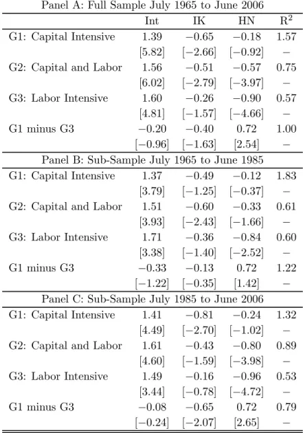
Table IV reports the results for the FMB cross-sectional regressions across firms grouped by capital intensity. The full sample results presented in Panel A confirm the hypothesis that the predictive power of the hiring and the investment rates varies with the firm’s capital and labor intensity. In both cases, the slope coefficients are negative but the magnitude and the statistical significance of the coefficient varies across each type of firm. As conjectured, only the investment rate has predictive power for stock returns within capital intensivefirms whereas for labor intensive
firms, only the hiring rate has predictive power. The t-test for the difference in the slope coefficient for thesefirms (G1 minus G3) confirm statistically that the difference in the slope coefficient across the capital intensive and the labor intensive group of firms is statistically significant, especially in the more recent sample period (Panel C).
[Insert Table IV here]
Turning to the analysis of the stock return predictability across industries, Table V reports the full sample FMB cross-sectional regression results across five industries. In computing these regressions, we require that each industry specific cross-section has at least 15 firms in order to estimate the industry specific slope coefficients with sufficient precision. As before, the regression produces negative average slopes for the hiring and investment rates across all industries. More interestingly, the results show some variation in the predictive power of hiring and investment rates across industries. Focusing on the full sample period results in Panel A, the investment rate is a significant predictor of returns in the manufacturing and high-tech sectors, whereas the hiring rate is significant return predictor in the consumer, manufacturing and high-tech sectors. Consistent with the analysis in the previous section, the predictability of the hiring rate is particularly strong in the more recent sample period in which the hiring rate is a statistically significant predictors of returns in all the industries considered (at the 10% level in the health-care sector). Taken together, the results in this section suggest that the sensitivity of thefirm’s future returns to the investment and hiring rates varies across technologies.
[Insert Table V here]
C.3 Relationship With Other Anomalies
In this section we examine if the investment and hiring rate maintain its predictive power after controlling for a broader set of stock return predictors. In choosing the set of return predictors, we follow Fama-French (2008). In addition to the standard size, book-to-market and momentum char-acteristics, we examine asset growth, net stock issues, positive accruals, and positive profitability.9 These additional anomaly variables are the statistically significant predictors of returns reported in Fama-French (2008), table IV, row "All but Micro". We considerfive empirical specifications which differ in the set of return predictors included. We consider size, book-to-market and momentum in all specifications and in specifications one to four we consider one the previous additional anomaly variables separately. Finally, in the last specification we consider all anomaly variables together.
The first specification in Table VI, Panel A reports the full sample results when the asset growth characteristics is included. The slope coefficient associated with asset growth is negative and statistically significant as in Fama-French (2008) and in the original Cooper, Gulen and Schill
9
The use of the asset growth characteristic follows from the work of Cooper, Gulen and Schill (2008). The use of the net stock issues characteristic follows from the work of Ikenberry, Lakonishok, and Vermaelen (1995), Loughran and Ritter (1995), Daniel and Titman (2006) and Pontiffand Woodgate (2006). The use of the accruals characteristics folows from the work initiated by Sloan (1996). Finally, the use of the profitability characteristic follows from the work of Haugen and Baker (1996) and Cohen, Gompers, and Vuolteenaho (2002).
(2008). Comparing with the previously reported results in Table III, Panel A, we note that the presence of the asset growth variable decreases the slope coefficient associated with investment and hiring in half. This is expected since, as documented in Table I, both the investment and hiring rate are significantly correlated with asset growth. Interesting however, the hiring rate is still a significant predictor of returns after controlling for asset growth. But the asset growth characteristic seems to drive out the investment rate factor.
[Insert Table VI here]
Specifications two to four in Table VI, Panel A report the full sample results when the net stock issues, positive accruals and positive profitability are included separately. The estimated slope coefficients associated with these variables produces the sign previously documented in the literature. High net stock issues and accruals are associated with low future returns, whereas high values of profitability are associated with high future returns. Impressively, both the investment and the hiring rate maintain its predictive power when each anomaly variable is included, despite the decrease in the magnitude of the associated investment and hiring rate slope coefficients. Only when all anomalies variables are included together (last specification) the investment and hiring rate loose their marginal predictive power. This result is not surprising given the well decomunented predictive power for stock returns of all these anomaly variables.
D
Portfolio Approach
We now turn to a portfolio approach to investigate the predictive content of the investment and the hiring rate for stock returns. We examine the characteristics of nine portfolios double sorted on hiring and investment rates. In constructing these portfolios, we follow Fama and French (1993). In each June of yeart, wefirst sort the universe of common stocks into three portfolios based on the firm’s hiring rate (cutoffs at the 33th and 66th percentile) at the end of year t-1. Then, each one of these three hiring portfolios are then equally sorted into three portfolios based on their investment rate (cutoffs at the 33th and 66th percentile) at the end of year t−1. Once the portfolios are formed, their value and equally weighted returns are tracked from July of year t to June of year t+1. The procedure is repeated in June of year t+1. For tractability, we only study portfolios using the whole sample of firms and do not investigate the variation across groups of firms as we did in the previous section.
[Insert Table VII here]
Table VII reports mean characteristics for each portfolio. Except for returns, all characteristics are measured at the time of the portfolio formation. Consistent with the results from the FMB regressions, the value weighted and the equally weighted average excess returns are decreasing in both the investment and hiring rates. The sorting procedure generates an impressive spread in the average excess returns of these portfolios. For example, the low investment rate-low hiring rate portfolio (low-low) has a value weighted excess return of 8.37% in the data whereas the high
investment rate-high hiring rate portfolio (high-high) has a value weighted excess return of only 1.32%(a difference of7.05%per year). This difference is even more impressive for equally weighted returns (9.7%per year). The characteristics of these portfolios also reveal that the book-to-market ratio (BM) is significantly negatively correlated with the average investment and hiring rates of these portfolios whereas and Asset Growth (AG) are positively correlated with the average investment and hiring rates. These variables have been found to be strong predictors of future returns by previous research (see, for example, the summary provided in Fama and French, 2008) and thus the large spread in the returns of these portfolios is consistent with these previousfindings.
In order to investigate if the spread in the average returns across these portfolios reflects a compensation for risk (at least as measured by standard risk factors), we conduct time series asset pricing tests using the CAPM and the Fama French (1993) model as the benchmark asset pricing models. In testing the CAPM, we run time series regressions of the excess returns of these portfolios on the market excess return portfolio while in testing the Fama-French three factor model we run time series regressions of the excess returns of these portfolios on the market excess return portfolio (Market), the SMB and the HML factors. We then examine the alphas (intercepts) of these regressions which are a measure of abnormal return. If the spread in the average returns of these portfolios is indeed a compensation for risk, then the alpha of these portfolios should be jointly zero. We test this prediction by the Gibbons, Ross and Shanken (Gibbons, Ross and Shanken ,1989) GRS test of the hypothesis that the alphas are jointly zero.
[Insert Table VIII here]
Table VIII, Panel A reports the asset pricing test results for the CAPM and for the Fama French (1993) model using both equally weighted and the value weighted portfolios and for the whole sample period. The CAPM is clearly rejected on both the equally weighted and value weighted portfolios by the GRS test (p-val of 0.00% and p-val of 5.03% respectively). The reason for this rejection follows from the fact that the spread in the unconditional CAPM market beta across these portfolios is too small relative to the spread in the average excess returns. Thus the model generates large statistically significant alphas for some portfolios, especially for the high-high portfolio. The returns on this portfolio clearly represent a puzzle for the CAPM. This portfolio behaves as a risky stock as measured by its high market beta but the realized average returns on this portfolio are very small. The poorfit of the CAPM on these portfolios can also be seen in the top panel in Figure 2, which plots the realized versus the predicted excess returns implied by the estimation of the CAPM on these portfolios. The straight line in each panel is the 45◦ line, along which all the assets should lie. The deviations from this line are the alphas (pricing errors). As a result of the low spread in betas, most portfolios lie along a vertical line and the high-high portfolio (portfolio 33 in the picture) is a clear outlier.
[Insert Figure 2 here]
The test results for the Fama French (1993) asset pricing model presented in Table VIII are better. The model is rejected in equally weighted portfolios by the GRS test (p-val of 0.01%) but
it’s not rejected on value weighted portfolio (p-val of 37.1%).10As in the CAPM, the returns on the high-high equally weighted portfolio represent a puzzle for the Fama French model. This portfolio behaves as a risky-value stock as measured by its high market and HML beta but the realized average returns on this portfolio are too small even considering its low (negative) SMB beta. The relative better fit of the Fama French model on these portfolios and the difficulty in pricing the high-high portfolio (portfolio 33) can also be seen in the plot of the pricing errors from this model presented in the right panel of Figure 2. In this picture, most portfolios lie along the45◦ degree line and the high-high portfolio is again an outlier. These results are robust. We obtain qualitatively similar conclusions when the Carhart (1997) momentum factor is included, when we examine an asset pricing model that includes a factor mimicking portfolio of the aggregate unemployment rate (following the evidence presented in Boyd, Hu and Jagannathan (2005)), the aggregate labor income growth factor (following the evidence presented in Jagannathan and Wang (1996)), or when the returns of these portfolios are measured net of the return on a matching portfolio formed on size and book-to-market equity (the portfolio adjusted average returns are similar to the intercepts on the three Fama-French factors time series regressions).
Taken together, the unconditional asset pricing test results presented in this section are con-sistent with the hypothesis that the firm betas are time varying. The unconditional CAPM beta is unable to capture the variation in the returns on these portfolios. The Fama French model is more successful at capturing the variation in the returns across these portfolios, but the model still leaves the returns on the high-high portfolio as a puzzle to be explained.
II
The Theoretical Link Between Hiring, Investment and Stock
Returns
In this section we propose a production-based asset pricing model that links thefirm’s hiring and investment rates to the firm’s stock return. The purpose of the model is to provide a theoretical justification for the use of the investment and hiring rate as predictors of stock returns and to un-derstand the economic driving forces that underlie the empirical evidence presented in the previous section. We show that the firm’s hiring and investment rate are proxies for the firm’s conditional beta. As a test of the story proposed by our model, in section III we provide a simulation of the model and verify that the model can replicate the empirical facts well.
A
Model
We consider an economy composed of a large number offirms that produce an homogeneous good. Here, we consider the production decision problem of one firm in this economy. This firm uses capital kt and labor nt to produce output yt and is subject to adjustment costs when changing
1 0
We not that the non rejection of the Fama-French model on value weighted portfolios is not robust across periods. In a sub-sample from 1975 to 2006, the Fama-French model is rejected on both equally weighted and value weighted portfolios. In this sub-sample, the misspricing of the high-high portfolio is even more pronounced than in the full sample (alpha of the high-high portfolios is statistically significant). Results are available upon request.
these inputs along the lines of Merz and Yashiv (2007). Thefirm is competitive and takes as given the market-determined stochastic discount factor Mt+1 used to value the cash-flows arriving in periodt+ 1, the stochastic wage rateWt+1 and the stochasticfirm level productivityext+zt, where
xt is an aggregate shock and zt is a firm specific shock.11 These stochastic variables are assumed
to be correlated but we postpone the specification of the stochastic processes of these variables to the simulation of the model section (section III) since the exact specification does not play a direct role on the results in this section.
Define the vector of state variables as st = (kt, nt, Wt, Mt, xt, zt) and let Vcum(st) be the cum
dividend contingent claim value of thefirm in period t. Thefirm makes investmentitand hiringht
decisions in order to maximize the cum dividend present value of the firm by solving the problem
Vcum(st) = max it+j,ht+j,j=1..∞E t ⎡ ⎣X∞ j=0 Mt,t+j+1dt+j ⎤ ⎦ (1)
subject to the constraints,
dt = yt−Wtnt−it−g(it, ht, kt, nt)−f (2)
yt = ext+ztf(kt, nt) (3)
nt+1 = (1−δk)nt+ht (4)
kt+1 = (1−δn)kt+it (5)
k0, n0 given
for all datestand where we useEt[.]to represent the expectation over all states of nature given all
the information available at time t. We focus on an all-equityfinancedfirm and therefore we model the dividendsdt in(2)as consisting of outputyt, less the wage billWtnt, investmentit, adjustment
costs of investment and hiring which are summarized by the function g(it, ht, kt, nt), and a fixed
cost of production f. A negative dividend is considered as equity issuance. Total output is given by (3) where f(kt, nt) is a standard production function that is increasing and concave in both
arguments. The law of motion for the capital and labor stock in (5) and (4) has a standard form except that the stock of labor is assumed to decline at an exogenous separation or ’attrition’ rate of δn, as in Shapiro (1984). The capital stock is assumed to depreciate at a rate of δk. As in Merz
and Yashiv (2007), the adjustment cost function g(it, ht, kt, nt) is homogeneous of degree one in
its arguments and is increasing and convex in the investment and hiring rate and decreasing and convex in the capital and labor stock.
1 1The existence of a strictly positive stochastic discount factor is guaranteed by a well-known existence theorem if
A.1 Decomposition of Firm’s Market Value and Stock Return
The first order conditions for thefirms’ maximization problem are given by
1 +git = Et[Mt,t+1(ykt+1+ (1−δk)−gkt+1+ (1−δk)git+1)] (6)
ght = Et[Mt,t+1(ynt+1−Wt+1−gnt+1+ (1−δn)ght+1)] (7) where we use the notation gitto denote the first partial derivative of the function g with respect to
the variable i, and similarly for the other variables. Thefirst order conditions (6) and (7) establishes a link between the exogenous stochastic discount factor, the exogenous wage rate and the firms’ investment and hiring decisions. The left hand sides of these equations are the marginal cost of investment and the marginal cost of hiring, respectively. The right sides of these equations are the risk adjusted discounted marginal benefit of investment and hiring, respectively. At the optimum, the firm chooses a level of investment and hiring such that the marginal costs and the marginal benefits are equalized.
To simplify the notation, define qtk and qnt as the marginal costs of investment and hiring (the investment marginal q and the hiring marginal q), respectively:
qkt ≡ 1 +git (8)
qtn ≡ ght (9)
To facilitate the exposition, we will assume for now that the production function f(.) has constant returns to scale (CRS) and we set the fixed costs of production to zero. Even though we will assume decreasing returns to scale and positive fixed costs of production in the simulation section of the model, these additional assumptions allows us to establish a link between the firm’s value, thefirm’s stock return and thefirm’s investment and hiring rates in closed form. Following Merz and Yashiv (2007), we show in Proposition 1 that in this setup, the market value of thefirm reflects the market value of the two inputs (capital and labor) used in the production of thefirm’s output. This result is simply an extension of Hayashi’s (1981) result to a multi factor inputs setting.
Proposition 1 (Merz and Yashiv (2007), Hayashi (1981)) When thefirm’s production and adjustment cost functions are both homogeneous of degree one (constant returns to scale) andfixed costs of production are zero, the ex dividend market value of the firm Vtexequals the sum of the market value of capital and market value of labor
Vtex= qktkt+1 | {z }
Market value of capital
+ qtnnt+1 | {z },
Market value of labor
where qtk≡1 +git and qtn≡ght are the marginal costs of investment and hiring respectively.
Intuitively, Proposition 1 states that the factor inputs are valued at their replacement costs, which in our setup are given by the marginal cost of investment and hiring (qtkandqnt). Because of the existence of labor adjustment costs, the marginal cost of hiring is typically non-zero, and thus a component of the market value of thefirm is attributed to labor. This result is in sharp contrast with the results from standard q theory with no adjustment costs in labor (qn
t ≡0), in which the
market value of the firm only reflects the value of thefirms’ stock of capital.
The decomposition of the market value of thefirm can be extended to establish a link between between thefirm’s stock return and thefirm’s investment and hiring rates, as stated in Proposition 2. To make the link more transparent, we proceed by specifying a functional form for the adjustment cost function. The results in this section hold for any homogeneous of degree one production and adjustment cost function. The functional form for adjustment costs function that we explore in this paper is g(it, ht, kt, nt) = ci 2 µ it kt ¶2 kt+ ch 2 µ ht nt ¶2 nt (10)
where ci and ch are constants. This specification is the natural generalization of the quadratic
investment adjustment cost specification popular in the q-theory of investment literature.12
Proposition 2 When the firm’s production and adjustment cost functions are both homogeneous of degree one (constant returns to scale) and fixed costs of production are zero, the firm’s stock return is given by Rst+1= q k t+1kt+2+qtn+1nt+2+dt+1 (1 +cikitt)kt+1+chhnttnt+1 (11) where qk
t ≡ 1 +cikitt and qtn ≡ chhntt are the marginal costs of investment and hiring respectively.
The expected stock market return can then be expressed as
Et £ Rst+1¤= Et £ qk t+1kt+2+qtn+1nt+2+dt+1 ¤ (1 +cikitt)kt+1+chhnttnt+1 (12)
Proof. Equation(11)follows directly from the defintion of stock returnRst+1 = V
e x
t+1+dt+1
Ve x
t and from Proposition 1, Vtex =qtkkt+1+qntnt+1. To go from (11) to (12) we use the fact that (11) holds ex post state by state and thus it also holds ex ante in expectation.
1 2
This specification differes from Merz and Yashiv (2007) who allow adjustment costs to hiring and investment to interact in order to capture the idea that simultaneous hiring and investment is less costly than sequential hiring and investment of the same magnitude because simultaneous action by the firm is less disruptive to production than sequential action. For tractability, we omit the interaction term from our exposition since, for reasonable calibrations, the interaction term does not change the qualitative implications of the model for the link between stock return predictability and thefirm investment and hiring rates that we explore in this paper.
A.2 The Link Between the Firm’s Investment Rate, Hiring Rate and Conditional Beta
Proposition 2 shows that characteristics are sufficient statistics for expected returns since the mar-ginal costs of investment and hiring as well as the firms’ dividends are a function of firm charac-teristics only. This interesting result is familiar from the investment-based asset pricing models of Cochrane (1991 and 1996), Liu, Whited and Zhang (2007) and Li, Livdan and Zhang (2008) for example. To understand the link between characteristics, firm beta and expected stock returns, we follow Cochrane (2005, p.14-16) and Chen and Zhang (2007) and re-write equation (12) in beta-pricing form:
Et£Rst+1 ¤
=Rtf+βtλmt (13)
whereqkt ≡1+cikitt ,qtn≡chhntt,Rft is the risk-free rate,βt≡ −Covt
¡
Rst+1, Mt+1 ¢
/Var(Mt+1) is the amount of risk, and the price of risk is given byλmt ≡Var(Mt+1)/Et[Mt+1]. Combining equations (12) and (13) yields βt= Ã Et £ qtk+1kt+2+qnt+1nt+2+dt+1 ¤ (1 +cikitt)kt+1+chnhttnt+1 − Rft ! /λmt (14)
which trivially links the firm’s conditional beta to firm characteristics. This result shows that a characteristic-based interpretation and a risk-based interpretation of expected returns are in fact the two sides of the same coin, as discussed extensively in Liu, Whited and Zhang (2007) and Chen and Zhang (2007), for example. In particular, characteristics can be seen as proxies for thefirm’s conditional beta (a risk-based explanation). In empirical work however, characteristics-based models are likely to outperform covariance-characteristics-based models. As discussed in Chen and Zhang (2007), this observation follows naturally from the fact that in a world with time varying betas, characteristics are more precisely measured than covariances, an observation that Gomes, Kogan and Zhang (2003) confirm in simulated data. Thus the use offirm level characteristics such as the investment and the hiring rate is supported theoretically by the fact that these characteristics are proxies for firm’s time varying conditional beta.
III
Model Predictions from a Simulation Economy
The firm’s stock return decomposition established in Propositon 2 can be used to understand the driving forces behind expected stock returns. By providing a link between firm level investment, hiring and stock returns, Proposition 2 allows us to to interpret the facts in the data. The analysis of this relationship is complicated however, because the investment and hiring rate are endogenous variables in the model. Thus a simple differentiation analysis of thefirm’s equilibrium stock return decomposition(12)with respect to the investment and hiring rate is not an appropriate procedure to evaluate the model implied relationship between stock returns and investment and hiring rates. To address this question, we create artificial data by simulating the theoretical model and investigate
the quantitative implications concerning the cross section of returns. We simulate 100 samples, each with 3600firms and 50 annual observations. The empirical procedure on each artificial sample is implemented and the cross-simulation results are reported. We also replicate the portfolio approach by constructing nine double-sorted portfolios sorted on investment and hiring rate and examine if the model can replicate the failures of the CAPM and the better fit of the Fama French (1993) model. Appendix A-3 provides a detailed description of the solution algorithm and the numerical implementation of the model.
A
Stochastic Processes and Functional Forms
Production requires two inputs, capital, k, and labor,l, and is subject to both an aggregate shock,
x, and an idiosyncratic shock,z. The aggregate productivity shock has a stationary and monotone Markov transition function, denoted byQx(xt+1|xt), and follows the following process:
xt+1 = ¯x(1−ρx) +ρxxt+σxεxt+1, (15) whereεxt+1 is an IID standard normal shock. The idiosyncratic productivity shocks, denoted byzj,t,
are uncorrelated acrossfirms, which we index by j, and have a common stationary and monotone Markov transition function, denoted byQz(zj,t+1|zj,t), and follows the following process:
zj,t+1=ρzzj,t+σzεzj,t+1, (16)
where εzj,t+1 is an IID standard normal shock and εzj,t+1 and εzi,t+1 for any pair (i, j) with i 6= j. Moreover, εxt+1 is independent ofεzj,t+1 for all j. In the model, the aggregate productivity shock is the driving force of economic fluctuations and systematic risk, and the idiosyncratic productivity shock is the driving force of the cross-sectional heterogeneity offirms.
The production function is decreasing returns to scale:
yt=ext+zj,tkαtkn αn
t , (17)
whereyt is output.
Following Berk, Green and Naik (1999) and Zhang (2005), we directly specify the pricing kernel without explicitly modeling the consumer’s problem. The pricing kernel is given by
logMt,t+1 = logβ+γt(xt−xt+1) (18)
γt = γ0+γ1(xt−x¯) , (19)
whereMt,t+1denotes the stochastic discount factor from timettot+ 1. The parameters{β, γ0, γ1} are constants satisfying 1> β >0, γ0 >0 and γ1<0.
Equation (18) can be motivated as a reduced-form representation of the intertemporal marginal rate of substitution for a fictitious representative consumer or the equilibrium marginal rate of transformation as in Cochrane (1993) and Belo (2008). Following Zhang (2005), we assume in
equation (19) that γt is time varying and decreases in the demeaned aggregate productivity shock
xt−x¯to capture the countercyclical price of risk with γ1<0.13
The equilibrium wage rate Wt is assumed to be an increasing function of the aggregate shock
xt
Wt=wexp(xt). (20)
withw >0.
B
Calibration
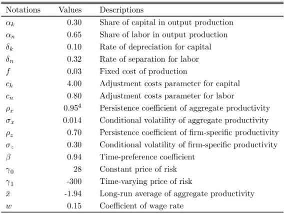
We calibrate parameters at annual frequency based on existing empirical evidence as well as by matching known aggregate asset pricing facts. Table IX presents these parameters. The first set of parameters specifies the technology of the firm. The second set of parameters describes the exogenous stochastic processes that the firm faces. The first three parameters are relatively uncontroversial and we set them according to exiting empirical estimates. We set the capital intensity parameter toαk= 0.3and the labor intensity parameter toαn= 0.65in the Cobb-Douglas
production function (17), which are close to the labor share parameters specified in Gomes(2001) for a CRS technology. The capital depreciationδk to be 10% a year as in Jermann (1998), and the
labor force attrition to be 32% equivalent to Merz and Yashiv’s (2007) 8% quarterly separation rate and consistent with the estimate of labor flows in Burgess Lane and Stevens (2000). We set the persistence of aggregate productivity shock ρx = 0.954 and conditional volatility σx = 0.007×2,
which corresponds to the quarterly estimates in Cooley and Prescott (1995). The long-run average level of aggregate productivity,x,¯ is a scaling variable. Following Zhang (2005), we set the average long-run capital in the economy at one, which implies that the long-run average of aggregate productivity x¯ = −1.93. To calibrate persistence ρz and conditional volatility σz of firm-specific
productivity, we follow Gomes (2001) and Zhang (2005) and restrict these two parameters using their implications on the degree of dispersion in the cross-sectional distribution of firms’ stock return volatilities. Thus ρz = 0.70, and σz = 0.30, which implies an average annual volatility of
individual stock returns of 24.4%, approximately the average of 25% reported by Campbell at al (2001) and 32% reported by Vuolteenaho (2001).
Following Zhang (2005), we pin down the three parameters governing the stochastic discount factor, β, γ0,and γ1 to match three aggregate return moments: the average real interest rate, the volatility of the real interest rate, and the average annual Sharpe ratio. This procedure yields
β = 0.94, γ0 = 28,and γ1 =−300,which generate an average annual real interest rate of 1.20%, an annual volatility of real interest rate of 5.8%, an average annual Sharpe ratio of the model is 0.33.
The rest of the parameters are not so straightforward to choose. In particular, the cost of adjustment parameters are very controversial. Estimates in the investment literature range from 20 in Summers (1980), to 2 in Whited (1993) to not significantly different from 0 in Hall (2001). The
1 3
The precise economic mechanism driving the countercyclical price of risk is, e.g., time-varying risk aversion as in Campbell and Cochrane (1999).
costs of adjusting labor are also controversial. Most of the literature assumes they are insignificant, while direct estimates suggests they can be substantial (Hamermesh (1993) and Merz and Yashiv (2007)). We therefore set the adjustment cost parameters by calibrating the model to be consistent with recent estimates of labor and capital adjustment cost functions (Merz and Yashiv (2007)) and with features of the USfinancial markets. In particular we look for parameters that are consistent with a 5-8% equity premium. Specifically, we set the parameter ck = 4 which in the middle of
the range of emprical estimates, and we set cn = 0.8 since Merz and Yashiv estimated that ck is
about four to six times bigger than cn.We estimate the parameter w in the wage process Wt to
be0.20. In order to gurrentee thatfirms market value of equity is increasing in labor in the state space, we setw= 0.15.And thefixed cost of production is set atf = 0.03by matching the average book-to-maket ratio.
Table X reports the unconditional moments of well known moments from the simulated and the real data. The model matches quantitatively the mean and volatility of the risk free rate, the risk-premium and the average gross investment and net hiring rates in the data. The sharpe ratio implied by the model is slightly higher than the Sharpe ratio in the data and the average book to market is slighlty lower. The major difficulty of the model is in replicating the volatility of the investment and hiring rates which are too low in the model. In addition, the model generates a correlation between then investment and hiring rate that is too high relative to the correlation in the data.
C
Properties of the Model Solutions
C.1 The Value Function and Policy Functions
Using the numerical solution to the benchmark model, we plot and discuss the value and policy functions as functions of the underlying state variables. Because there are four state variables (cap-ital stock kt, labor stock nt, the aggregate productivity shock xt, and idiosyncratic productivity
shockzt), and the focus of the paper is the cross-sectional variations, we fix the aggregate
produc-tivity shock at its long-run average, xt= ¯x.Figure 3, Panels A and C plot the variables againstkt
and zt,with nt and xt fixed at their long-run average levels n¯ and x¯. Panels B and D in Figure 3
plot the variables against nt and zt, with kt and xt fixed at their long-run average level ¯k and x.¯
Each one of these panels has a set of curves corresponding to different values ofzt,and the arrow
in each panel indicates the direction along which zt increases.
[Insert Figure 3 here]
In Panels A and B in Figure 3, the firm’s cum-dividend market value of equity is increasing in the firm-specific productivity, the capital stock and the labor stock. In Figure 3, Panels C and D, the optimal investment and hire are increasing in the firm-specific productivity. This indicates that the more profitable firms with higherfirm-specific productivity invest and hire more than less profitable firms with lower firm-specific productivity. This finding is consistent with the evidence
documented by Fama and French (1995). In Figure 3, Panels C and D, the optimal investment rates and hire rates are decreasing in capital stocks and labor stock, respectively. Smallfirms with less capital invest and hire more and grow faster than bigfirms with more capital and more labor. That prediction is consistent with the evidence provided by Evans (1987) and Hall (1987).
C.2 Fundamental Determinants of Risk
Wefind that risk, measured asβtfrom equation (14), is decreasing in the three firm-specific state variables: the capital stock, the labor stock and thefirm-specific productivity. Using the benchmark parametrization, Panels E and F of Figure 3 plot βt against physical capital,kt, and labor stock,
nt,andfirm-specific productivity,zt, with the aggregate productivityfixed at its long-run averages,
xt= ¯x.Doing so allows us to focus on the cross-sectional variation of risk. Panels E and F plotβt
in four curves, each of which corresponds to one value of firm-specific productivity,zt. The arrow
in the panels indicates the direction along which zt increases. Small firms with less capital and
less labor are more risky than bigfirms with more capital and more labor. That is consistent with Li, Livdan and Zhang (2007). Consistent with Zhang (2005), less profitable firms are riskier than more profitable firms
D
Can the Model Replicate the Empirical Findings?
D.1 Stock Return Predictability and Hiring and Investment Rates
The main empirical fact established in this paper is that the current hiring rate, in addition to the current investment rate, is negatively correlated with future stock returns. The model can replicate the negative slope of the FMB coefficients remarkably well. Figure 4, Panels A and B plot the histogram of the estimated FMB slope coefficients associated with the investment rate and the hiring rate respectively, and Figure 4 Panel C plot the joint histogram of the investment and hiring rate slope coefficients. As the figures shows, the empirical FMB slope coefficients are well inside the distribution of the FMB slope coefficients generated by the model. The estimated average slopes in the simulated model are thus close to the empirical estimates. For the investment rate, the simulated average FMB slope is -0.85 which is slighlty higher than the empirical slope of -0.45. For the hiring rate the fit is better. The simulated average FMB slope is -0.56 which is virtually identical to the empirical slope of -0.57.
[Insert Figure 4 here]
D.2 Stock Return Predictability Across Firms With Different Technologies
In the data, future stock returns of capital intensive firms are more sensitive to variations in the investment rate than to variations in the hiring rate and the opposite was true for labor intensive firms. In addition, there is substantial variation in the predictive power of the investment and hiring rate across industries. We use the model to explore two potential explanations for this pattern. The first explanation is based on differences in the labor intensity parameter in the production function