Bi-directional Tracking using Trajectory Segment Analysis
Jian Sun
Weiwei Zhang
Xiaoou Tang
Heung-Yeung Shum
Microsoft Research Asia, Beijing, P. R. China
{
jiansun, weiweiz, xitang, and hshum
}
@microsoft.com
Abstract
In this paper, we present a novel approach to keyframe-based tracking, called bi-directional tracking. Given two object templates in the beginning and end-ing keyframes, the bi-directional tracker outputs the MAP (Maximum A Posterior) solution of the whole state se-quence of the target object in the Bayesian framework. First, a number of 3D trajectory segments of the object are extracted from the input video, using a novel trajectory ment analysis. Second, these disconnected trajectory seg-ments due to occlusion are linked by a number of inferred occlusion segments. Last, the MAP solution is obtained by trajectory optimization in a coarse-to-fine manner. Exper-imental results show the robustness of our approach with respect to sudden motion, ambiguity, and short and long pe-riods of occlusion.1
Introduction
Visual tracking is one of the fundamental problems in com-puter vision. Given the observations, i.e. a video sequence, tracking infers the states of the target object(s). Applica-tions range from video surveillance, human-computer inter-faces, and augmented reality to digital video editing.
Most tracking approaches work in a recursive way:
es-timating object location at the current timetbased on the
observations up to time t. In a Bayesian framework, the
tracking problem is commonly formulated as a recursive
es-timation of a time-evolving posterior distributionP(xt|y1:t)
of statextgiven all the observationsy1:t. Recursive
estima-tion has two major advantages: 1) it is efficient in computa-tion, and 2) it naturally fits into real-time or online tracking applications.
Many real world applications such as event statistics in video surveillance, object-based video compression, home video editing, video annotation, and visual motion capture can be regarded as offline tracking where all the frames from the input video sequence can be used. In offline tracking, moreover, a long video sequence can be decomposed into short ones by specifying a few keyframes, which is also called keyframe-based tracking. Each keyframe contains an object template which can be given by hand or by using some automatic object detection methods.
To utilize the information from these keyframes, a straightforward method is to apply the recursive approach from keyframes going forward or backward. One problem of this approach is that when tracking fails in the middle of the sequence, we have to add another keyframe at the
failed location. However, it is very difficult to predict when the method may fail, thus we have to add the keyframe in a trial-and-error manner which is prohibitively time consum-ing. The second problem is that the recursive method only uses information in one keyframe while ignoring informa-tion in the other keyframe.
Recent work on rotoscoping [1] tracks the contours in video for animation using user-specified contours in two or more frames. Rotoscoping makes full use of the informa-tion in the keyframes to improve the performance of contour tracking. However, rotoscoping is limited to tracking only parameterized curves, which is difficult to apply to other tracking applications.
In this paper, we develop a bi-directional tracking al-gorithm of generic objects by taking advantage of the in-formation in both keyframes. Formally, given a video
se-quence and two statesx1andxT in the beginning and
end-ing keyframes, we compute the MAP solution of the whole state sequence:
P(x2:T−1|y1:T, x1, xT)∼P(y1:T|x1:T)P(x2:T−1|x1, xT)
(1) The success of our algorithm depends on whether it can overcome the following two challenges.
One challenge is to provide an efficient optimization al-gorithm to obtain the MAP solution. In visual tracking, the whole continuous state sequence space usually has an enor-mous number of local minimums due to nonlinear dynam-ics and non-gaussian observations. Gradient-based meth-ods will often become stuck at a local minimum. The MAP solution can be also computed by Viterbi algorithm using a discrete HMM (Hidden Markov Model) representation. However, the the quantized state space is very large even
for a simple state representation for a320×240video.
The other challenge is to handle partial or complete oc-clusions. Short-time occlusions can often be handled by an appropriate dynamics model. However, for more complex occlusions, such as long-time occlusions or occlusions by similar objects, previous methods often fail. How to han-dle various difficult occlusions using the information in two keyframes is of both theoretical and practical interest in the bi-directional tracking.
In order to overcome the above difficulties, our bi-directional tracking uses a novel trajectory segment repre-sentation. Trajectory segments are a number of small frac-tions of possible object trajectories in the 3D video volume.
Trajectory segments are extracted from the input video us-ing a spectral clusterus-ing method. With this representation, the MAP solution can be efficiently obtained in a coarse-to-fine manner by a discrete HMM model. More important, at the trajectory segment level, we propose an occlusion rea-soning algorithm to robustly infer possible occlusion trajec-tory segments of the target object.
2
Previous Work
Tracking remains a very difficult vision problem due to sev-eral reasons, for example sudden motion, ambiguity and oc-clusion. The sudden motion of object may be caused by unexpected dynamic changes of the object itself or abrupt camera motion. When the target object comes close to a similar object, tracking algorithms often fail to locate the correct one due to ambiguity. The target object may be par-tially or completely occluded. Occlusion can be of short or long. A number of approaches have been proposed to alleviate these problems.
Direct optimization The direct optimization ap-proaches [12, 2, 7, 4] estimate the motion parameters between two neighboring frames by minimizing a deter-ministic cost function. The direct optimization approach assumes slow motion between two frames. This kind of approach is efficient but not very robust in situations with rapid sudden motion, ambiguity, and long-time occlusion.
Particle filtering Condensation [10] is the first particle
fil-tering [6, 11] based algorithm introduced in visual tracking. Particle filtering approximates the posterior distribution us-ing a set of “weighted particles”. The particle filterus-ing algo-rithm has advantages on handling sudden motion and short-time occlusion. However, it often difficult to handle am-biguity or long-time occlusion. Maccormick & Black pro-posed a “probabilistic exclusion principle” [13] to address the ambiguity problem. But their approach is limited to a special observation model for contour tracking.
Offline tracking Offline tracking exploits all the
informa-tion in the video sequence. In [9], the optical flow over the entire sequence is estimated simultaneously using a rank constraint on the rigid motion. Torresani & Bregler [17] track 3D points using a low rank constraint on a 3D morphable model and importance sampling in trajectory space. Multiple hypothesis tracking (MHT) was proposed by Reid [16] and improved by Cox & Hingorani [5] for mul-tiple objects tracking. They give a Bayesian formulation for determining the probabilities of measurement-to-target as-sociation hypotheses. Recent work in [8] optimizes a MAP solution of the joint trajectories of objects for multiple ob-ject tracking. Their approach severely relies on background substraction and object detection, and no explicit occlusion reasoning mechanism is presented.
3
Framework
In this paper, we chose a very basic state model and ob-servation model to demonstrate our bi-directional tracking approach in the keyframe-based framework.
State The target object is represented as a rectangleR =
{p, s∗w, sb ∗bh}, wherepis the center rectangle andsis the
scaling factor. wbandbhare a fixed width and height of the
object template, respectively. So, we denote the state of the
object asx= {p, s} ∈ X, whereX is the state space. In
the bi-directional tracking, the statex1in the first keyframe
I1and the statexT in the last keyframeIT are known.
Observation The observation is the color statistics of the
target object. The object’s color model is represented as
a histogram h = {h1, ..., hH} with H (typically, H =
8×8×8) bins in RGB color space. The Bhattacharyya
dis-tance between the associated histogramh(x0)of the state
x0and the associated histogramh(xi)of the statexiis
de-fined as: B2[h(x
0),h(xi)] = 1−PBj=1
p
hj(x0)hj(xi).
This model only captures global color statistics. A more so-phisticate multi-part color model [15] can be used if there is a certain spatial configration of the target object.
Trajectory Optimization The posterior of the whole state
sequenceX = {x2, ..., xT−1} for a given video sequence
Y = {y1, ..., yT} and known two states{x1, xT} can be
represented as follows under the first order Markov inde-pendence assumption: P(X|Y, x1, xT) = 1 Z T−1 Y i=2 ψ(yi|xi, x1, xT) T−1 Y i=1 ψ(xi, xi+1), (2)
where the local evidenceψ(yi|xi, x1, xT)is defined using
the Bhattacharyya distance:
ψ(yi|xi, x1, xT)∼exp(−min{B2[h(xi),h(x1)],
B2[h(x
i),h(xT)]}/2σh2),(3)
whereσ2
his the variance parameter. It measures the
similar-ity between the color histogramh(xi)of the statexito the
closest color histogram betweenh(x1)in the keyframesI1
orh(xT)inIT. The potential functionψ(xi, xi+1)between
two adjacent states is defined as:
ψ(xi, xi+1)∼exp(−D[xi, xi+1]/2σ 2
p), (4)
whereD[xi, xi+1] =||pi−pi+1||2+β||si−si+1||2is the
similarity between statexiandxj. σpis a variance to
con-trol the strength of smoothness andβ is a weight between
location difference and scale difference. It is a smoothness constraint on the whole trajectory of the target object.
The goal of the bi-directional tracking is to obtain the MAP solution of Equation (2). To efficiently perform the optimization and handle possible occlusion, we present a novel approach based on trajectory segment analysis. Fig-ure 1 shows the basic flow of our approach:
Trajectory Segment Analysis Occlusion Reasoning Trajectory Optimization
(Section 4) (Section 5) (Section 6)
Figure 1:Flowchart of bi-directional tracking.
1. Trajectory segment analysis. For a given video se-quence and object templates in two keyframes, trajec-tory segment analysis extracts a number of small 3D trajectory segments in the video volume using a spec-tral clustering method.
2. Occlusion reasoning. To handle both short-time and long-time occlusions, we connect disjointed trajectory segment pairs where an occlusion segment may exist in between.
3. Trajectory optimization. A number of discrete states in each frame are sampled from the segments obtained in step 2. The MAP solution of Equation (2) is obtained by a discrete HMM model in a coarse-to-fine manner.
4
Trajectory Segment Analysis
Trajectory segment analysis consists of two steps: 2D mode
extraction in each frame independently and 3D trajectory segment extraction in the whole video simultaneously.
4.1
2D mode extraction
The purpose of 2D mode extraction is to significantly re-duce the whole state space so that further analysis on a sparse state set is tractable. For each frame, we can com-pute an evidence surface using Equation (3). The 2D modes are peaks or local maxima on this surface. A 2D mode
rep-resents a state x′ whose observation is similar to the
ob-ject templates in the keyframes. Namely, the local evident
ψ(y|x′, x
1, xT)is high.
To efficiently find these modes, we adopt the mean shift [4] algorithm which is a nonparametric statistical method seeking the nearest mode of a point sample distrib-ution. Given an initial location, mean shift can compute the gradient direction of the convoluted evidence surface by a
kernelG[4]. With this property, the mean-shift algorithm
is a very efficient iterative method for gradient ascent to a local mode of the target object.
To perform 2D mode extraction, we uniformly sample the location in the image and the scale (3-5 discrete lev-els) to obtain a set of starting states. The spatial sampling interval is sightly smaller than half the size of the object. Then, the mean shift algorithm runs independently from each starting state. After convergence, we get a number
of local modes. Finally, we reject the state modex′ whose
local evidenceψ(y|x′, x
1, xT)≤0.5and merge very close
modes to generate a sparse set of local 2D modes in each frame, as shown in the bottom row of Figure 2.
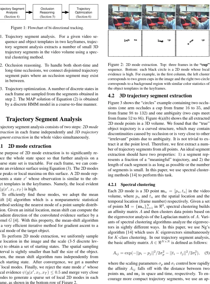
Figure 2: 2D mode extraction. Top: three frames in the “cup”
sequence. Bottom: each black circle is a 2D mode whose local evidence is high. For example, in the first column, the left cluster corresponds to two green cups in the image and the right two circle corresponds to a background region with similar color statistics of the object templates in the keyframes.
4.2
3D trajectory segment extraction
Figure 3 shows the “circles” example containing two
occlu-sions (one arm occludes a cup from frame16 to35, and
from frame98to132) and one ambiguity (two cups meet
from frame52to86). Figure 4(a)(b) shows the all extracted
2D mode points in a 3D volume. We found that the “true” object trajectory is a curved structure, which may contain discontinuities caused by occlusion or is very close to other “irrelevant” points due to ambiguity. It is not trivial to ex-tract it at the point level. Therefore, we first exex-tract a num-ber of trajectory segments from all points. An ideal segment extraction should have two properties: 1) a segment rep-resents a fraction of a “meaningful” trajectory, and 2) the length of each segment is as long as possible or the number of segments is small. In this paper, we use spectral cluster-ing methods [14] to perform this task.
4.2.1 Spectral clustering
Each 2D mode is a 3D pointmn = [pn, tn] in the video
volume, wherepn andtn are the spatial location and the
temporal location (frame number) respectively. Given a set
of pointsM= {mn}Nn=1inℜ
3, spectral clustering builds
an affinity matrixAand then clusters data points based on
the eigenvector analysis of the Laplacian matrix ofA.
Vari-ants of spectral clustering algorithms analyze the eigenvec-tors in sightly different ways. In this paper, we use Ng’s
algorithm [14] which usesK eigenvectors simultaneously
forK-class clustering. In our trajectory segment analysis,
the basic affinity matrixA∈ ℜN×N is defined as follows:
Aij = exp(−||pi−pj||2/2σp2− ||ti−tj||2/2σ2t), (5)
where the scaling parametersσpandσtcontrol how rapidly
the affinity Aij falls off with the distance between two
pointsmiandmj in space and time, respectively. To
ap-pearance dependent definition in this paper:
A′ij =αAij+ (1−α) exp(−B2[h(mi),h(mj)]/2σh2),
(6) where the last term measures the similarity between the
ap-pearances (color histogram in this paper) of two modes.αis
a weighting factor (typically0.5). The process to partition
the points intoKclusters is as follows:
1. Build the affinity matrixAaccording to Equation (6).
2. Construct the matrixL=D−1/2
AD−1/2
whereDis
a diagonal matrix (Dii =PNj=1Aij).
3. Compute the matrixE= [e1, ..., eK]∈ ℜN×K, where
ekis the normalizedKlargest eigenvectors ofL.
4. Treat each row of E as a point in ℜK, and cluster
them intoK clusters by K-means algorithm. Assign
the original point to clusterk if rowi of the E was
assigned to clusterk.
After spectral clustering, we treat all 3D points in clusterk
as a trajectory segmentT rk. Namely, we get a number of
Ktrajectory segmentsTr ={T r1, ..., T rK}. Figure 4(e)
shows the extracted trajectory segments on the “circles” se-quence. Spectral clustering successfully produces a number of “meaningful” trajectory segments.
4.2.2 Why use spectral clustering?
We get less “meaningful” results from a standard k-means clustering. The reason is that the “true” trajectory is usu-ally highly curved and some partition of it may not be a convex region, but every cluster of k-means has to be a con-vex region. Figure 4(a)(b) shows two k-means results using
different scaling factors of the time variablet. In fact, we
found that k-means always gives unsatisfactory results no matter what the scaling factor is for this example.
In contrast, in spectral clustering, 3D data points are
em-bedded on the surface of a unit sphere in anotherK
dimen-sional space spaned by theKlargest eigenvectors ofL. In
this space, curved trajectories or manifolds in the original 3D space can be well separated. Clustering in the embed-ded space using spectral analysis is the key to our trajectory segment analysis. We refer the reader to [14, 3] for more details and comparisons.
5
Occlusion Reasoning
If there is no occlusion of the target object, trajectory seg-ments extraction is already a very good “proposal” for state space sampling in trajectory optimization. However, due to partial or complete occlusion occurring in the input video, the occlusion (trajectory) segment (the states during occlu-sion stage) does not exist in already extracted segments. The occlusion segment should be inferred and sampled be-tween object trajectory segments. This section presents a
simple but effective occlusion reasoning algorithm at the trajectory segment level.
After analyzing the trajectory segments on a number of video sequences, we have several observations:
A. The trajectory segment including object templates in the keyframes must be in the “true” object trajectory. B. The trajectory segment parallel to the segment which
contains object templates should be excluded. C. No occlusion segment exists between two overlapping
trajectory segments along the time axis.
D. There are certain speed and time limits on an occlusion segment.
In observation B, two segments are parallel if the overlap-ping time and the shortest distance between them are not more than certain empirical thresholds. For example, in Figure 4(e) the vertical segment (red) in the center will be excluded because it is parallel to two segments (cyan and dark-green) containing object templates.
5.1
Occlusion reasoning algorithm
Based on the above observations, we propose an bi-directional, tree-growing algorithm for occlusion reasoning as follows:
1. Build two treesTA andTB. Each tree has an empty
root node. Then, add one trajectory segment contain-ing an object template in the keyframe to each tree as an active node. The remaining segments are denoted as a candidate set.
2. Exclude the trajectory segment from the candidate set using the current two trees according to observation B.
3. For each active leaf-node (node without child) inTA,
add theQ-best occlusion segments from the candidate
set or the active leaf-nodes inTB as its child nodes,
according to observations C and D. The newly added child node is set to active if it comes from the candidate set. Otherwise, it is set to inactive in both trees.
4. The treeTBgrows one step in a similar way.
5. If there is no active leaf-node in both trees, stop; oth-erwise, go step 2.
Occlusion trajectory generation For two disjoint
trajec-tories T r1 and T r2 in time, we want to fill in the
miss-ing occlusion segmentO in between, as shown in Figure
5. Given all points{mj= [pj, tj]}N
′
j=1inT r1andT r2, we
fit a B-spliner(s) =PNB
n=0Bn(s)qnusing weighted least
squares: min {qn} XN′ j=1w(mj)||r(s ′ j)−mj||2, (7) wheres′ j = (tj−t1)/N′is a temporal parametrization of
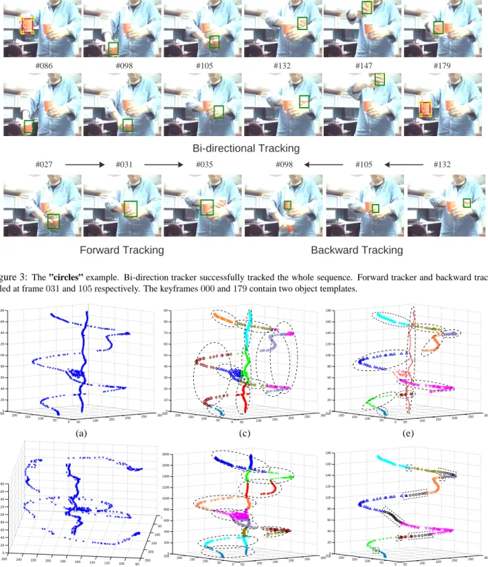
#016 #027 #065 #086 #105 #132 #000 #147 #179 #035 #052 #098 #027 #031 #035 #098 #105 #132 Bi-directional Tracking
Forward Tracking Backward Tracking
Figure 3: The ”circles” example. Bi-direction tracker successfully tracked the whole sequence. Forward tracker and backward tracker
failed at frame031and105respectively. The keyframes000and179contain two object templates.
50 100 150 200 250 300 0 50 100 150 200 2500 20 40 60 80 100 120 140 160 180 50 100 150 200 250 300 0 50 100 150 200 2500 10 20 30 40 50 60 70 80 90 50 100 150 200 250 300 0 50 100 150 200 2500 20 40 60 80 100 120 140 160 180 (a) (c) (e) 80 100 120 140 160 180 200 220 240 260 0 50 100 150 200 250 0 20 40 60 80 100 120 140 160 180 50 100 150 200 250 300 0 50 100 150 200 2500 200 400 600 800 1000 1200 1400 1600 1800 50 100 150 200 250 300 0 50 100 150 200 2500 20 40 60 80 100 120 140 160 180 (b) (d) (f)
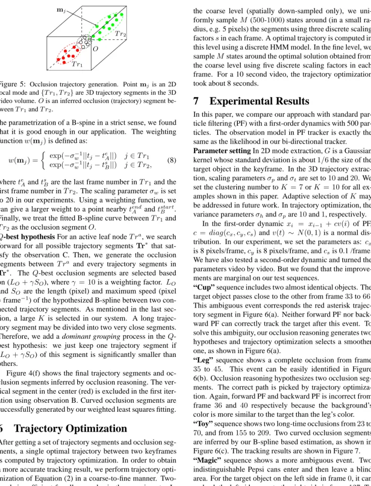
Figure 4: Trajectory segments analysis on ”circles” sequence. (a)(b) two views of all 2D mode points in 3D. The vertical axis is the
frame number in the sequence. (c)(d) two k-means results with different time scaling factors. K-means does not provide very meaningful ”segments” in terms of trajectory. (e) meaningful ”segments” from spectral clustering. (f) result after occlusion reasoning. Black circles in dashed rectangles are filled-in occlusion segments. Please view the electronic version for a better illustration in color.
mj
T r1
T r2
O
Figure 5: Occlusion trajectory generation. Pointmj is an 2D
local mode and{T r1, T r2}are 3D trajectory segments in the 3D
video volume.Ois an inferred occlusion (trajectory) segment be-tweenT r1andT r2.
the parametrization of a B-spine in a strict sense, we found that it is good enough in our application. The weighting
functionw(mj)is defined as:
w(mj) = exp(−σ−1 w ||tj−teA||) j∈T r1 exp(−σ−1 w ||tj−tsB||) j∈T r2, (8) wherete
AandtsB are the last frame number inT r1and the
first frame number inT r2. The scaling parameterσwis set
to 20 in our experiments. Using a weighting function, we
can give a larger weight to a point nearbytend
A andtstartB .
Finally, we treat the fitted B-spline curve betweenT r1and
T r2as the occlusion segmentO.
Q-best hypothesis For an active leaf nodeT ra, we search
forward for all possible trajectory segments Tr∗ that
sat-isfy the observation C. Then, we generate the occlusion
segments between T ra and every trajectory segments in
Tr∗. The Q-best occlusion segments are selected based
on (LO+γSO), whereγ = 10is a weighting factor. LO
andSO are the length (pixel) and maximum speed (pixel
∗frame−1) of the hypothesized B-spline between two
con-nected trajectory segments. As mentioned in the last
sec-tion, a largeK is selected in our system. A long
trajec-tory segment may be divided into two very close segments.
Therefore, we add a dominant grouping process in theQ
-best hypothesis: we just keep one trajectory segment if
(LO +γSO) of this segment is significantly smaller than
others.
Figure 4(f) shows the final trajectory segments and oc-clusion segments inferred by ococ-clusion reasoning. The ver-tical segment in the center (red) is excluded in the first iter-ation using observiter-ation B. Curved occlusion segments are successfully generated by our weighted least squares fitting.
6
Trajectory Optimization
After getting a set of trajectory segments and occlusion seg-ments, a single optimal trajectory between two keyframes is computed by trajectory optimization. In order to obtain a more accurate tracking result, we perform trajectory opti-mization of Equation (2) in a coarse-to-fine manner. Two-levels is sufficient for all examples in the experiments. In
the coarse level (spatially down-sampled only), we
uni-formly sampleM (500-1000) states around (in a small
ra-dius, e.g. 5 pixels) the segments using three discrete scaling
factorssin each frame. A optimal trajectory is computed in
this level using a discrete HMM model. In the fine level, we
sampleMstates around the optimal solution obtained from
the coarse level using five discrete scaling factors in each frame. For a 10 second video, the trajectory optimization took about 8 seconds.
7
Experimental Results
In this paper, we compare our approach with standard ticle filtering (PF) with a first-order dynamics with 500 par-ticles. The observation model in PF tracker is exactly the same as the likelihood in our bi-directional tracker.
Parameter setting In 2D mode extraction,Gis a Gaussian
kernel whose standard deviation is about1/6the size of the
target object in the keyframe. In the 3D trajectory
extrac-tion, scaling parametersσpandσtare set to10and20. We
set the clustering number toK = 7orK = 10for all
ex-amples shown in this paper. Adaptive selection ofK may
be addressed in future work. In trajectory optimization, the
variance parametersσhandσpare10and1, respectively.
In the first-order dynamic xi = xi−1 +cv(i) of PF,
c = diag(cx, cy, cs)andv(t) ∼ N(0,1)is a normal
dis-tribution. In our experiment, we set the parameters as: cx
is 8 pixels/frame,cyis 8 pixels/frame, andcsis 0.1 /frame.
We have also tested a second-order dynamic and turned the parameters video by video. But we found that the improve-ments are marginal on our test sequences.
“Cup” sequence includes two almost identical objects. The
target object passes close to the other from frame33to66.
This ambiguous event corresponds the red asterisk trajec-tory segment in Figure 6(a). Neither forward PF nor back-ward PF can correctly track the target after this event. To solve this ambiguity, our occlusion reasoning generates two hypotheses and trajectory optimization selects a smoother one, as shown in Figure 6(a).
“Leg” sequence shows a complete occlusion from frame
35 to 45. This event can be easily identified in Figure
6(b). Occlusion reasoning hypothesizes two occlusion seg-ments. The correct path is picked by trajectory optimiza-tion. Again, forward PF and backward PF is incorrect from
frame 36 and 40 respectively because the background’s
color is more similar to the target than the leg’s color.
“Toy” sequence shows two long-time occlusions from23to
70, and from155to209. Two curved occlusion segments
are inferred by our B-spline based estimation, as shown in Figure 6(c). The tracking results are shown in Figure 7.
“Magic” sequence shows a more ambiguous event. Two
indistinguishable Pepsi cans enter and then leave a blind
area. For the target object on the left side in frame0, it can
0 50 100 150 200 250 300 80 100 120 140 160 180 200 220 0 20 40 60 80 100 80 100 120 140 160 180 200 220 240 50 100 150 200 0 5 10 15 20 25 30 35 40 45 50 0 50 100 150 200 250 300 0 100 200 0 50 100 150 200 250 300 0 50 100 150 200 250 300 80 100 120 140 160 180 200 220 0 20 40 60 80 100 80 100 120 140 160 180 200 220 240 50 100 150 200 0 5 10 15 20 25 30 35 40 45 50 0 50 100 150 200 250 300 0 100 200 0 50 100 150 200 250 300
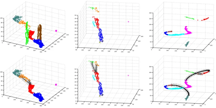
(a) Cup (b) Leg (c) Toy
Figure 6: Trajectory segments analysis results (Top) and occlusion reasoning results (Bottom). The black circles in dash rectangles are
inferred occlusion segments. (a) two segments corresponding to the cup in the center and a green region on the background are excluded. (b) two possible occlusion segments are hypothesized. (c) two highly curved occlusion segments are estimated.
solve this ambiguity, our bi-directional tracker can give two reasonable guesses by specifying two kinds of keyframes, as shown in Figure 7.
8
Conclusion
In this paper, we have presented a bi-directional tracking ap-proach based on trajectory segment analysis. Curved target object trajectories are successfully extracted by trajectory segment analysis and connected by the occlusion reasoning algorithm. With a trajectory segment representation, more challenging visual tracking tasks can be well handled.
There are many opportunities to improve and general-ize our approach, such as automatic selection of clustering number, handling large appearance changes between two keyframes, integrating more visual cues, developing other state representations, and bi-directional tracking of multi-ple objects.
References
[1] A. Agarwala, A. Hertzmann, D. Salesin, and S. Seitz. Keyframe-based tracking for rotoscoping and animation. In Proceedings of
SIGGRAPH 2004, 2004.
[2] S. Birchfield. Elliptical head tracking using intensity gradients and color histograms. CVPR, 1998.
[3] M. Brand and K. Huang. A unifying theorem for spectral embedding and clustering. Proceedings of Inte. Conf. on AI and Statistics, 2003. [4] D. Comaniciu, V. Ramesh, and P. Meer. Real-time tracking of
non-rigid objects using mean shift. CVPR, 2000.
[5] I.J. Cox and S.L Hingorani. An efficient implementation of reid’s multiple hypothesis tracking algorithm and its evaluation for the pur-pose of visual tracking. IEEE Tran. on PAMI., 8(2):138–150, 1996. [6] N. J. Gordon, D. J. Salmond, and A. F. M. Smith. Novel approach to
nonlinear/non-gaussian bayesian state estimation. IEE Proceedings
on Radar and Signal Processing., 140:107–113, 1993.
[7] G.D. Hager and P.N. Belhumeur. Efficient region tracking with para-metric models of geometry and illumination. IEEE Tran. on PAMI, 20(10):1025–1039, 1998.
[8] M. Han, W. Xu, H. Tao, and Y. H. Gong. An algorithm for multiple object trajectory tracking. CVPR, 2004.
[9] M. Irani. Multi-frame optical flow estimation using subspace con-straints. ICCV, 1999.
[10] M. Isard and A. Blake. Contour tracking by stochastic propagation of conditional density. ECCV, 1996.
[11] J. Liu and R. Chen. Sequential monte carlo methods for dynamic systems. J. Amer. Statist. Assoc., 93:1032–1044, 1998.
[12] B. Lucas and T. Kanade. An iterative image registration technique with an application to stereo vision. Proceedings of the Int. Joint
Conf. on AI., pages 593–600, 1981.
[13] J. MacCormick and A. Blake. A probabilistic exclusion principle for tracking multiple objects. ICCV, 1999.
[14] A. Y. Ng, M. Jordan, and Y. Weiss. On spectral clustering: Analysis and an algorithm. NIPS, 2002.
[15] P. P´erez, C. Hue, J. Vermaak, and M. Gangnet. Color-based proba-bilistic tracking. ECCV, 2002.
[16] D.B. Reid. An algorithm for tracking multiple targets. IEEE Tran.
on Automatic Control, 24(6):843–854, 1979.
#33 #48 #99 #00 #66 #83 #33 #66 #66 #18 #18 #48 #26 #36 #49 #00 #40 #45 #36 #40 #46 #26 #32 #40 #023 #045 #086 #000 #061 #070 #155 #178 #257 #114 #209 #226 #015 #062 #127 #000 #089 #110
Figure 7: “Cup”, “Leg”, “Toy”, and “Magic” examples (from top to bottom). In “cup” and “leg” examples, we compare bi-direction