Using word embeddings in Twitter election classification

Yang, X., Macdonald, C. and Ounis, I. (2018) Using word embeddings in

Twitter election classification. Information Retrieval, 21(2-3), pp. 183-207.

(doi:

10.1007/s10791-017-9319-5

)

This is the author’s final accepted version.

There may be differences between this version and the published version.

You are advised to consult the publisher’s version if you wish to cite from

it.

http://eprints.gla.ac.uk/150070/

Deposited on: 20 December 2017

Enlighten – Research publications by members of the University of Glasgow

http://eprints.gla.ac.uk

Xiao Yang · Craig Macdonald · Iadh Ounis

Accepted: 3 October 2017; Author’s version.

Abstract Word embeddings and convolutional neural networks (CNN) have attracted extensive attention in various classification tasks for Twitter, e.g. sentiment classifica-tion. However, the effect of the configuration used to generate the word embeddings on the classification performance has not been studied in the existing literature. In this paper, using a Twitter election classification task that aims to detect election-related tweets, we investigate the impact of the background dataset used to train the embed-ding models, as well as parameters of the word embedembed-ding training process, namely the context window size, the dimensionality and the number of negative samples, on the attained classification performance. By comparing the classification results of word embedding models that have been trained using different background corpora (e.g. Wikipedia articles and Twitter microposts), we show that the background data should align with the Twitter classification dataset both in data type and time period to achieve significantly better performance compared to baselines such as SVM with TF-IDF. Moreover, by evaluating the results of word embeddings models trained us-This manuscript extends a paper previously made available on arXiv (https://arxiv.org/abs/1606.07006) entitled “Using Word Embeddings in Twitter Election Classification”, and presented at the Workshop on Neural Information Retrieval at SIGIR 2016. This is an author’s version of DOI:10.1007/s10791-017-9319-5, accepted to be published in the Information Retrieval Journal. The final publication is available at https://link.springer.com. This work is supported by a grant from the Economic and Social Research Council (ES/L016435/1).

X. Yang

School of Computing Science University of Glasgow, UK E-mail: [email protected] C. Macdonald

School of Computing Science University of Glasgow, UK

E-mail: [email protected] I. Ounis

School of Computing Science University of Glasgow, UK E-mail: [email protected]

ing various context window sizes and dimensionalities, we found that large context window and dimension sizes are preferable to improve the performance. However, the number of negative samples parameter does not significantly affect the perfor-mance of the CNN classifiers. Our experimental results also show that choosing the correct word embedding model for use with CNN leads to statistically significant im-provements over various baselines such as random, SVM with TF-IDF and SVM with word embeddings. Finally, for out-of-vocabulary (OOV) words that are not available in the learned word embedding models, we show that a simpleOOVstrategy to ran-domly initialise theOOV words without any prior knowledge is sufficient to attain a good classification performance among the currentOOV strategies (e.g. random initialisation using statistics of the pre-trained word embedding models).

1 Introduction

Word embeddings have been proposed to produce effective word representations. For example, in theWord2Vecmodel [23], by maximising the probability of seeing a word within a fixed context window, it is possible to learn for each word in the vocabulary a dense real valued vector from a shallow neural network. As a conse-quence, similar words are close to each other in the embedding space [4, 9, 23], such as “quick” and “quickly” that are syntactically similar. However, word embeddings can provide more complex semantic relationships by applying algebraic operations to certain word vectors. For example, Mikolov et al. [24] observed that a simple al-gebraic operationvector(“King”)−vector(“Man”)+vector(“Woman”)results in a vector that is closest to the vector representation of “Queen”. A similar example is to find the country that a city belongs to, such as “France” is to “Paris” what “China” is to “Beijing”. Such semantic relationships are useful for various tasks such as infor-mation retrieval [25], named entity tagging [15], text classification [18] and machine translation [22].

However, a common issue of using word embeddings is the out-of-vocabulary (OOV) words that appear in datasets but not in word embedding models. Thus, the vector representations of theOOVwords cannot be obtained from the learned word embedding model. There are several existingOOV strategies in the existing litera-ture. For example, Kim [18] used the statistics from learned word embedding models to randomly initialise the vector representations for theOOVwords. On the contrary, OOVwords were ignored by both Bojanowski et al. [6] and Mitra et al. [25]. Dhingra et al. [11] proposed character-based distributed representations which learn embed-dings for each character rather than word, and therefore vectors forOOVwords are resolved at the character level. However, there has been little exploration of which strategy is better at dealing with theOOV words from the word level, and indeed both Kim [18] and Mitra et al. [25] suggested that further study on theOOV strate-gies for word embedding models is needed.

Recently, the use of word embeddings together with convolutional neural net-works (CNN) has been shown to be effective for various classification tasks such as sentence classification [18] and sentiment classification on Twitter [13, 28]. In such approaches, word embeddings are used to construct the vector representation of a

sentence or a tweet as the input of a CNN classifier. In order to investigate the effect of different CNN settings in sentence classification performance, a sensitivity anal-ysis of a one-layer CNN classifier has been conducted by Zhang et al. [37] through varying the hyperparameters such as the filter region size, the number of feature maps and the pooling strategy. However, the effect of the configuration used to generate the word embeddings on the classification performance has not been studied in the liter-ature. Indeed, while different background corpora (e.g. Wikipedia and Twitter) and parameters (e.g. context window and dimensionality) could lead to different word embeddings, there has been little exploration of how such background corpora and parameters affect the classification performance.

In this paper, using two Twitter datasets collected during the Venezuela parlia-mentary election in 2015 and the Philippines general election in 2016 respectively, we investigate the use of word embeddings with CNN in a new classification task, which aims to identify those tweets that are related to the election. Such a classifi-cation task is challenging because election-related tweets are usually ambiguous and it is often difficult for human assessors to reach an agreement on their relevance to the election [5]. For example, such tweets may refer to the election implicitly without mentioning any political party or politician. In order to tackle these challenges, we propose to use word embeddings to build richer vector representations of tweets for training the CNN classifier on our election dataset.

Our contributions are three-fold: First, we thoroughly investigate the parame-ter settings (e.g. context window, the dimensionality and negative sample size) of word embeddings on our election classification task. We show that word embed-dings trained using a large context window size and dimension size can help CNN to achieve significantly better classification performance over our baselines (e.g. SVM with TFIDF). Second, we explicitly study the effect of the background corpus. Our results show that when the type and time period of background corpus align with the classification dataset, the CNN classifier achieves statistically significant im-provements over the classification baseline of SVM with TF-IDF on our task. Third, we compare several random strategies to addressOOV words. Our results on two datasets demonstrated that simpler OOV strategies to randomly initialise theOOV words without any prior knowledge is sufficient to attain a good classification per-formance among the current OOV strategies Thus, our results suggest indeed that the background corpus and parameters of word embeddings have an impact on the classification performance. Moreover, our results contradict the findings of differ-ent tasks such as dependency parsing [3] and named differ-entity recognition (NER) [15] where a smaller context window is suggested. Such a contradiction suggests that the best setup of parameters such as the context window and dimensionality might differ from a task to another.

In the remainder of this paper, we explain the related work in Section 2. We de-scribe the CNN architecture used for our classification task in Section 3. In Section 4, we describe our dataset and the experimental setup. In Section 5, we investigate the impact of the context window size, dimensionality and negative sample size of word embeddings on the classification performance. In Section 6, we discuss the impact of two different types of background corpora (Wikipedia articles and Twitter microp-osts) on the effectiveness of the learned classifier. In Section 7, we study the strategies

that aims to deal with the out-of-vocabulary (OOV) words. We provide concluding remarks in Section 8.

2 Related work

In this section, we introduce related work in the areas of word embedding, Twitter classification and how they relate to the study presented in this paper.

2.1 Word embedding models

In most text classification tasks, terms within the documents are often used as features such as the classic TF-IDF vector representation. Word embedding models based on neural networks have emerged as an effective alternative to build vector represen-tations of text [4, 8, 21, 27]. The main aim of word embeddings is to learn vector representations of words by mapping semantic information into a geometric word embedding space. In these models, the vector representationw of a given word is usually learned through a fixed context windowW. In addition, to capture semantic information from the fixed context window, the recently proposedGloVemodel [27] also aims to capture global corpus statistics through the word co-occurrence proba-bilities. Another word embedding model, namelyWord2Vec[21, 23], maximises the conditional probability of a word given the context words that appeared around that word within the context windowW. After training, the learned vector representations wcan be used to reveal the relation between two words using their corresponding vector representationswiandwjand a similarity measure (e.g.cosinesimilarity):

sim(wi,wj) =cosine(wi,wj) =

wi·wj

||wi||||wj||

(1)

In particular, theWord2Vecmodel contains two separate embeddings, namely the input and output embeddings [25]. However, the output embedding is usually dis-carded in most applications [15, 18, 22]. To leverage both of the embeddings, Mitra et al. [25] proposed a dual word embedding model for document ranking by retaining the output embedding that is often discarded in other applications. Using thecosine similarity defined in Eq. (1), Mitra et al. [25] noted that words in a dual word em-bedding model are more likely related by topics (e.g. “yale” is close to “faculty”). Without retaining the outputs embeddings, words are more likely related by types (e.g. “yale” is close to “harvard”). In particular, Bansal et al. [3] and Pennington et al. [27] observed that the embedding parameters can also affect the type of generated word embeddings. This shows that word embeddings can exhibit different properties in various settings, which leads to our proposed study on the effect of the embed-ding parameters such as the context window sizeW on the resulting classification performance.

Embedding parameters

A number of studies have already shown that the context window and dimensionality of the used word embedding vectors can affect performance in various tasks such as dependency parsing [3] and named entity recognition (NER) [15]. For instance, us-ing publicly available corpora such as Wall Street Journals and Wikipedia, Bansal et al. [3] investigatedWord2Vecword embeddings in a dependency parsing task, which aims to provide a representation of grammatical relations between words in a sen-tence. By only varying the context window size from 1 to 10, their results on the accuracy of part-of-speech (POS) tagging showed that the context window size of Word2Veccan affect the type of the generated word embedding. In particular, they observed that a smaller context window gives a better performance on accuracy. In the named entity recognition (NER) task, Godin et al. [15] investigated three context window sizesW ={1,3,5} based on the accuracy of NER tagging. From their re-sults, they also reached a similar conclusion, namely that a smaller context window gives a better performance using theWord2Vecword embeddings when the model is trained from a large Twitter corpus containing 400 million tweets.

Using a subset of the semantic-syntactic word relationship test set, Mikolov et al. [23] investigated the dimensionality of theWord2Vec word embeddings and the size of background data. In the test set, word pairs are grouped by the type of rela-tionship. For example “brother-sister” and “grandson-granddaughter” are in the same relationship of “man-woman”. The accuracy is measured such that given a word pair, another word pair with the correct relationship should be retrieved. Using this ac-curacy measure, they noted that at some point increasing the dimensionality or the size of background data only provides slightly better performance. Therefore, they concluded that the dimensionality and background data size should be increased to-gether [23]. Mikolov et al. [23] also studied another parameter, namely the number of negative samples, which defines how many negative examples are randomly sampled from the corpus vocabulary to train the word embedding models. For example, for the context “the cat sits on the mat”, a negative sample will be a word (e.g. project) randomly sampled from the entire corpus, which is often irrelevant to the current context. Such negative examples help the word embedding model to differentiate the correct word relationships from noise (i.e. negative samples). Therefore, during train-ing, the model maximises the probabilities to real word relationships and minimises the probabilities to the noise words. Mikolov et al. [23] observed that a large nega-tive sample size is useful for small background corpora while for large corpora the negative sample size could be as small as 2−5. However, Mikolov et al. [23] only investigated theWord2Vecparameters using the GoogleNews background corpus.

The aforementioned studies provide a useful guide about the effect of the word embeddings configuration on performance in the specific applications they tackled, but their findings were obtained on tasks different from Twitter classification tasks. Hence, the question arises as whether such findings will generalise to classification tasks on Twitter, which is the object of our study in this paper.

2.2 Twitter classification

In fact, there is little work in the literature tackling the task of election classification on Twitter. However, similar classification tasks such as Twitter sentiment classifica-tion have been well studied [13, 28, 32]. In particular, word embeddings were recently used to build effective tweet-level representations for Twitter sentiment classifica-tion [28, 32]. For instance, in the SemEval-2015 Twitter Sentiment Analysis chal-lenge, Severyn et al. [28] proposed to use word embeddings learned from two Twitter corpora to build the vector representations of tweets. Using theWord2Vecmodel, de-fault parameter values such as context window size 5 and dimensionality 100 were ap-plied to train the word embedding. In their approach, one Twitter background corpus (50 million tweets) was used to train the word embedding, while another one (10 mil-lion tweets) containing positive and negative emoticons was used to refine the learned word embeddings using the proposed CNN classifier. The CNN classifier was then trained on the SemEval-2015 Twitter sentiment analysis dataset, which contains two subsets: phrase-level and message-level datasets. Each subset contains 5K+ and 9K+ training samples, respectively. The official ranking in SemEval-2015 showed that this system ranked 1st and 2nd on the phase-level dataset and the message-level dataset, respectively. However, Severyn et al. [28] focused on refining the word embeddings by using another Twitter corpus with emoticons to learn sentiment information, but did not study the impact of the background corpus and the chosen parameters on the classification performance.

In another approach based on the word embeddings model proposed by Collobert et al. [8], Tang et al. [32] proposed a variation to learn sentiment-specific word em-beddings (SSWE) from a large Twitter corpus containing positive and negative emoti-cons. Tang et al. [32] empirically set the context window size to 3 and the embedding dimensionality to 50. The SemEval-2013 Twitter sentiment analysis dataset, which contains 7K+ tweets was used to evaluate the effectiveness of their proposed ap-proach. Compared to the top system of the SemEval-2013 Twitter Sentiment Anal-ysis challenge, their approach of using an SVM classifier with SSWE outperformed the top system on the F1 measure. However, only the Twitter background corpus was used by Tang et al. [32], which contains 10 million tweets with positive and negative emoticons. On the other hand, the parameters of word embeddings such as the context window and dimensionality were not studied by Tang et al. [32], nor in the existing literature for Twitter classification tasks. In particular, the aforementioned studies do not address the out-of-vocabulary (OOV) words that are not appeared in the learned embedding model. As such, in this paper, we conduct a thorough investigation of word embeddings together with CNN on a Twitter classification task and explore the impact of both the background corpus, the context window, the dimensionality and the negative sample size of word embeddings andOOVwords on the classification performance.

Fig. 1 Convolutional neural network architecture for tweet classification. Adapted from [18].

3 The CNN model

For our Twitter election classification task, we use a simple CNN architecture de-scribed by Kim [18] as well as the one proposed by Severyn et al. [29] and high-lighted in Fig. 1. It consists of a convolutional layer, a max pooling layer, a dropout layer and a fully connected output layer. Each of these layers is explained in turn.

Tweet-level representation.The inputs of the CNN classifier are preprocessed tweets that consist of a sequence of words. Word embeddings play an important role in building the tweet-level representations. The semantic relations carried by word embeddings are helpful to find semantic similarities between tweets.

Using word embeddings, tweets are converted into vector representations in the following way. Assuming wi∈Rn to be the n-dimensional word embeddings

vec-tor of thei-th word in a tweet, a tweet-level representation for convolutional neural networks (denotedTCNN) is obtained by looking up the word embeddings and con-catenating the corresponding word embeddings vectors of the totalkwords:

TCNN=w1⊕w2⊕ · · · ⊕wk (2)

where⊕denotes the concatenation operation [18]. As suggested by Kim [18], for a word not appearing in a word embeddings (also known asout-of-vocabulary OOV), we generate its vector by sampling each dimension from the uniform distributions Ui[mi−si,mi+si], wheremiandsi are the mean and standard deviation of thei-th

dimension of the word embeddings. For training purposes, short tweets are padded to k– the length of the longest tweet – using a special token. The vector representation of each word is concatenated and stacked as illustrated in Fig. 1. Hence, the total dimension of the vector representationTCNNis alwaysk×n. Afterwards, the tweet-level representation will feed to the convolutional layer.

Convolutional layer.The convolutional layer consists of a set of learnable filters that are applied to the network inputTCNNusing convolution operations. Since the size of each filterFi∈Rm×n is usually smaller than TCNN, a filter aims to only

detect the presence of specific features or patterns. This is the core building block of convolutional neural networks, which helps the network to learn the important patterns no matter where they appear in a tweet [28]. In this layer, the filterFi∈

Rm×n is randomly initialised and applied to the tweet-level representation TCNN. By varying the size ofm, multiple filter sizes can be used to covermwords during

the convolution operation as shown in Fig. 1, where three filter sizes are illustrated in different colours. By this means, the network learns important features by considering two or more adjacent words together. In this layer, by varying another parameter, namely strides[19], we can shift the filters across sword embeddings vectors at each step. Therefore, a largersleads to less computation. By sliding the filters over mword vectors inTCNNusing stride s, the convolution operation produces a new feature mapcifor all the possible words in a tweet:

ci=f(Fi·TCNNi:i+m−1+bi) (3)

wherei:i+m−1 denotes the word vectors of wordito wordi+m−1 inTCNN.bi

is the corresponding bias term that is initialised to zero and learned for each filterFi

during training. In Eq. (3), f is the activation function. In this CNN architecture, we use a rectified linear function (ReLU) [16] as the activation function f since ReLU shows very promising performance in convolutional neural networks [14]. Its output is given by:

Out put=Max(0,Input) (4)

Therefore, the ReLU unit ensures its output is always positive.

Max pooling layer.A pooling layer aims to reduce the spatial size of features and the computation in the network. All the feature mapscifrom the convolutional layer

are then applied to the max pooling layer where the maximum valuecmax_i is extracted from the corresponding feature map. In this way, only the most salient features are kept. Afterwards, the maximum values of all the feature mapsciare concatenated as

the feature vector of a tweet.

Dropout layer.Dropout is a simple yet effective regularisation technique that is often used in neural networks [30]. It only keeps a neuron active with some prob-ability p (e.g. p=0.5) during training [18]. After training, p=1 is used to keep all the neurons active for predicting unseen tweets. We apply both dropout and the well-knownL2 regularisation technique to control overfitting.

Softmax layer.The fully connected softmax layer transforms the output scores of positive and negative classes into normalised class probabilities [18] using the softmax function: ˆ yi= ezi ∑1t=0ezt f or i=0,1, (5)

where ˆyi indicates the normalised probability of classi.zidenotes the output score

of classi. The value ofican only be 0 or 1 in our task since we aim to only classify tweets as “election-related” or “not election-related”, which is a binary classification task. Letybe a vector representing the true label distribution and ˆybe the vector of the normalised probabilities from the softmax layer, the cross-entropy cost function is defined as follows: loss(yˆ,y) =− 1

∑

Eq. (6) calculates the dissimilarity between the true label distributionyand the pre-dicted label distribution ˆy. During training, the weights of each layer are updated according to the calculated loss. Once a CNN classifier is trained from a training set, all of its parameters and learned weights are saved. Unseen tweets then can be classified by applying their tweet-level representations to the trained CNN classifiers.

4 Experimental setup

In this paper, we argue that the types of background corpora as well as the parameters of Word2Vec model could lead to different word embeddings and could affect the performance on Twitter classification tasks. In the following sections, we address three research questions using our Twitter election classification task:

– RQ1: For Twitter election classification task, do the CNN classifiers prefer differ-ent word embedding settings from other tasks (e.g. dependency parsing [3] and NER [15])?

– RQ2: By using the same type of background corpus as the dataset, does the learned word embedding model improve the classification performance?

– RQ3: For out-of-vocabulary (OOV) words, what particular strategy (e.g. random initialisation using statistics of the trained word embedding models) is pre-ferred to attain good classification performance?

Our experiments are tailored to conduct a thorough investigation of word em-beddings together with CNN on a Twitter classification task by addressingRQ1in Section 5,RQ2in Section 6 andRQ3in Section 7. The remainder of this section details our dataset (Section 4.1), our experimental setup and used word embedding models (Section 4.2), the used baselines (Section 4.3) and measures (Section 4.4)

4.1 Dataset

Our two manually labelled election datasets are sampled from tweets collected about the 2015 Venezuela parliamentary election (held on 06/12/2015) and the 2016 Philip-pines general election (held on 09/05/2016), respectively. Both of the datasets cover the period of one month before and after the election dates. We use the Terrier in-formation retrieval (IR) platform [20] and the DFReeKLIM [2] weighting model – designed for microblog search – to retrieve tweets related to selected query terms that were provided by social science experts (we list all our query terms in Table 1(a)). Only the top 7 retrieved tweets are selected for each query term on each of the 60 days, making the size of the collection realistic for human assessors to examine and label the tweets. The sampled tweets are merged into one pool and judged by 5 experts who label a tweet as: “Election-related” or “Not Election-related”. To determine the judging reliability, an agreement study was conducted for the Venezuela dataset using 482 random tweets that were judged by all 5 assessors. Using Cohen’skappa[7], we found a moderate agreement of 52% between all assessors. For tweets without a ma-jority agreement, an additional expert of Venezuela or Philippines politics was used to further clarify their categories. Therefore, we obtain a dataset with good quality hu-man labels. In total, our Venezuela election dataset consists of 5,747 Spanish tweets, which contains 9,904 unique words after preprocessing (stop-word removal & Span-ish Snowball stemmer). In our Philippines election dataset, there are 4,163 EnglSpan-ish tweets with a total 10,229 unique words after preprocessing (stop-word removal & English Snowball stemmer). Overall, both of our labelled election datasets cover sig-nificant events during the elections. For example, killing of opposition politician Luis

(a) Query terms used to retrieve tweets Query terms Venezuela Dataset eleccion,violencia,votar,pistola,armas,ametralladora,ataque electora,muerto,miedo,muerte,asesinato,disparar,fraude muere,delincuente,herido,agreden,asesinar,guachiman,protesta Philippines Dataset violence,attack,dead,fraud,assault,protest,intimidation,unrest gunshot,racial,die,kill,threat,vote buying,murder,corrupt terrorize,ambush,explosion,shoot,fire,harass,injure,burn selling vote,cheating,election

(b) Statistics of the labelled datasets

Language Election Non-Election Total # Words Venezuela Dataset Spanish 2,274 3,474 5,747 9,904 Philippines Dataset English 1,755 2,408 4,163 10,229

Table 1 Query terms and statistics of the datasets used in the experiments.

Diaz [1] in the 2015 Venezuela parliamentary election is observed in our Venezuela dataset. From the general statistics shown in Table 1(b), we observe that both datasets are unbalanced; the majority class (Non-Election) has more tweets than the minority class (Election).

4.2 Word embeddings

As part of our experiments, we train word embedding models on different background corpora. When training on Twitter data, we removed tweets with less than 10 words since such tweets contains less information and are often meaningless (e.g. only con-tain Twitter handles or are dominated by stopwords and emoticons) for training the word embeddings in our task. For consistency, we apply the same preprocessing, namely stop-word removal and stemmer (see Section 4.1), to all of the background corpora. Since the Venezuela dataset is in Spanish while the Philippines dataset is in English, we train both Spanish and English word embedding models for our experi-ments.

Spanish word embedding models

Our Spanish word embeddings are for use with the Venezuela dataset that contains an-notated tweets of the 2015 Venezuela parliamentary election (held on 06/12/2015). The word embeddings used in this paper are trained from three different background corpora:

– es-Wiki: a Spanish Wikipedia snapshot dated 02/10/2015.

– es-Twitter-general: a general Spanish Twitter data collected from 05/01/2015 to 30/06/2015, which does not align with the election period of the 2015 Venezuela parliamentary election.

– es-Twitter-time: a Spanish Twitter data collected from the period 01/11/2015 to 31/12/2015, which covers the election period of the 2015 Venezuela parlia-mentary election.

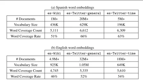
Over 1 million Spanish articles are observed in es-Wiki. After removing tweets with less than 10 words, over 20 million Spanish tweets are collected in the corpus

es-Twitter-general. In es-Twitter-time, over 5 million Spanish tweets are observed. After the preprocessing, thees-Wikicorpus contains 436K unique words,

es-Twitter-generalhas 629K unique words whilees-Twitter-timehas only 196K unique words. Salient statistics are provided in Table 2(a). Indeed, by compar-ing the unique words in our election dataset with the words in the three background corpora, we observe that 5,111 words in our dataset appear ines-Wiki, 6,612 words appear ines-Twitter-generalwhile 6,309 words appear ines-Twitter-time. This shows thates-Twitter-generalhas a better word coverage on our election datasets. We notice that es-Twitter-time has a very similar word coverage to

es-Twitter-generalthough it has a much fewer number of documents.

English word embedding models

Our English word embeddings are for use with the Philippines dataset that contains annotated tweets of the 2016 Philippines general election (held on 09/05/2016).

– en-Wiki: an English Wikipedia snapshot dated 02/10/2015

– en-Twitter-general: a general English Twitter data collected from 05/01/2015 to 23/03/2015, which does not align with the election period of the 2016 Philip-pines general election

– en-Twitter-time: an English Twitter data that is collected from the period 01/04/2016 to 31/05/2016, which covers the election period of the 2016 Philip-pines general election

For English word embedding corpora, over 4.9 million English articles are observed inen-Wiki, over 32 million English tweets in the corpus en-Twitter-general

and over 18 million English tweets are observed inen-Twitter-time. As shown in Table 2(b), the statistics of English word embeddings after the preprocessing, the

en-Wiki corpus contains 925K unique words,en-Twitter-general has 1.05M unique words while en-Twitter-timehas only 649K unique words. Similar to the Spanish word embedding models, by comparing the unique words in our Philip-pines election dataset with the words in the three English word embedding mod-els, we observe that en-Wiki has the lowest word coverage count, which shows that Twitter corpora have better word coverage on our election datasets. Hence, po-tentially the en-wiki model cannot work as well as en-Twitter-general and

en-Twitter-timedue to the low word coverage.

We use the Word2Vec implementation in deeplearning4j1 to generate a set of word embeddings by varying the context window sizeW, the dimensionalityDand the number of negative samplesns. We use context window sizesW ={1,5,10}to

(a) Spanish word embeddings

es-Wiki es-Twitter-general es-Twitter-time

# Documents 1M+ 20M+ 5M+

Vocabulary Size 436K 629K 196K

Word Coverage Count 5,111 6,612 6,309

Word Coverage Rate 51% 66% 63%

(b) English word embeddings

en-Wiki en-Twitter-general en-Twitter-time

# Documents 4.9M+ 32M+ 18M+

Vocabulary Size 925K 1.05M 649K

Word Coverage Count 4,745 5,335 5,610

Word Coverage Rate 46% 52% 54%

Table 2 Statistics of the background corpora used to train word embedding models and words coverage on the election datasets.

study both small and large context window sizes. For each context windowW, we use three different dimension sizesD={200,500,800}to study both of the low and high dimensionalities of the word embedding vectors. Therefore, 9 word embedding models in total are generated by varyingW andDfor bothes-Twitter-general

anden-Twitter-general. For other parameters, we use the same values that were set by Mikolov et al. [23]: We set the batch size to 50, negative sampling to 10, min-imum word frequency to 5 and iterations to 5. In addition, we also study the effect of the negative sample size on bothes-Twitter-generalanden-Twitter-general

by using negative sample sizesns={2,10}.

4.3 Baselines

To evaluate the CNN classifiers and word embeddings, we use four baselines, namely: Random classifier: According to the class distribution in the training set, the random classifier simply makes random predictions to the test instances.

SVM with TF-IDF (SVM+TFIDF): As a more sophisticated baseline than the

random classifier, the traditional weighting scheme, namely TF-IDF, is used in con-junction with an SVM classifier for the Twitter election classification.

SVM with word embeddings(SVM+WE): We use a similar scheme that was used

by Wang et al. [33] to build the tweet-level representation for the SVM classifiers. The vector representation (i.e.TW E) of a tweet is constructed by averaging the word embedding vectors along each dimension for all the words in the tweet:

TW E= k

∑

i=1

wi/k (7)

wherekis the number of words in a tweet andwi∈Rndenotes the word embedding

exactly the same dimension as the word embedding vectorwi, which is the input of an

SVM classifier. The concatenation scheme used in the CNN classifiers is not applied to the SVM classifiers because it gives worse performance according to our initial experiments. Indeed, a key advantage of the CNN classifier is to detect important patterns within a context window and the capture word order, attributes that cannot be captured using SVM with or without word embeddings.

fastText: As a state-of-the-art text classifier,fastTextprovides both effective and efficient learning of word representations and sentence classification [6, 17]. Based on theWord2Vecmodel,fastTextcan classify text documents using the word embeddings leaned from the given dataset. In addition, it also allows to useN-gramfeatures to capture some partial information about the local word order [17]. The efficiency and effectiveness offastTexthas been tested on several datasets (e.g. Yelp review dataset and Amazon review dataset). Compared to other systems [10, 31, 35, 36] using con-volutional neural networks and recurrent neural networks,fastTextshows comparable results but significantly less training time.

4.4 Hyperparameters and measures

To train the classifiers and evaluate their performances on our datasets, we use a 5-fold cross validation, such that in each fold, 3 partitions are used for training, 1 par-tition for validation and 1 parpar-tition for test. Afterwards, the overall performance on the test instances is assessed by averaging the scores across all folds. We report effec-tiveness in terms of classification measures, precision (denotedP), recall (denotedR) and F1 score (denotedF1). For statistical testing, we use the non-parametric McNe-mar’stest as proposed by Dietterich [12] for an computationally inexpensive method of hypothesis testing.

For all the experiments, we use 3 filter sizesm={1,2,3}, strides=1 and dropout probabilityp=0.5 for our CNN classifier, which gives better performance according to our initial experiments on the validation set. For each filter size, 200 filters are applied to the convolutional layer and therefore 600 feature maps are produced in total. For the SVM classifiers, we use theLinearSVCmodel inscikit-learn2[26] and tune the parametercfor each SVM classifier using the validation set. ForfastText3, the implementation provided by Joulin et al. [17] is used. We tune the dimensionality parameterdimto 200, theN-gramparameterwordNgramsto 2 and context window sizewsto 5, which attains good performance according to our initial experiments. For other parameters, such as learning rate, we use the default settings.

5 Effect of word embeddings parameters

In this section, we addressRQ1and investigate the effect of parameters (e.g. context window, dimensionality and negative samples) for the Twitter election classification task. As shown in Table 2, since word embedding modelses-Twitter-generaland

2 _{http://scikit-learn.org}

en-Twitter-generalhave good word coverage on our Venezuela and Philippines datasets respectively, we use them for all the experiments in this section.

5.1 Effect of context window and dimensionality

For Venezuela dataset, Table 3(a) shows the results of our four baselines, while Table 3(b) shows the results of classifiers using word embeddings, namely SVM with word embeddings (SVM+WE) and CNN. In Table 3(b), the measurements for SVM+WE and CNN are arranged by the dimensionality and context window size of word embeddings. For each row ofW1,W5 andW10, Table 3(b) shows results for context window sizes ofW ={1,5,10} along each dimension sizes of D=

{200,500,800}. The best overall scores are highlighted in bold. Table 4 has the same arrangement as Table 3 but shows the corresponding results for the Philippines dataset.

In Table 3(b), where both approaches (e.g. SVM+WE and CNN) use the same word embeddings, we observe that SVM+WE and CNN show similar preferences in word embeddings dimensionality. When we fix the context window size, SVM classifiers clearly show improvements on F1 score for all sizes ofW={1,5,10}by increasing the dimensionalityD. In particular, a larger dimensionalityD={500,800} results in better performances in terms of precision, recall and F1 scores compared to the embedding models with a smaller dimensionalityD=200. We observed sim-ilar results for the CNN classifiers. In particular, whenW ={5,10}, increasing the dimensionalityDimproves the recall and F1 scores.

Next, we study the effect of context window sizeW. If we fix the dimensionality Dwhile increasing the context window sizeW from 1 to 10, CNN classifiers show improvement on F1 score. In particular, larger context window sizesW ={5,10} also attain better recall compared to the embedding models usingW =1 whenD=

{500,800}. Similarly, the SVM classifiers also demonstrate improvements in recall and F1 when D=800 when increasing context window sizeW. In particular, by considering both the context window and dimensionality, SVM and CNN classifiers attain best performances in of terms of F1 scores whenW =10 andD=800. As such, the experimental results on Venezuela dataset show that a word embedding model with a higher context window size and dimensional is potentially the most appropriate for our task.

For the Philippines dataset, as shown in Table 4(b), we have observed similar results of the Venezuela dataset. By fixing context windowW and increasing the dimensionalityD, SVM classifiers clearly show improvements on all metrics. For CNN classifiers, the use of word embedding models with the largest dimensionality D=800 attains the best F1 score. Next, we study the effect of context window. If we fix the dimensionalityD={200,500}and increase the context windowW from 1 to 10, all metrics are improved for the SVM classifiers. We note that the size of context windowWdoes not affect the performance of the SVM classifiers much when D=800. However, the use of larger context window sizesW ={5,10}improves F1 score for CNN classifiers compared to a small window sizeW =1. In particular, the CNN classifier attains the best F1 score by using the word embedding model with

(a) Results of random classifier, SVM+TFIDF, SVM+WE andfastText

Precision Recall F1 score

Random* 38.6 28.5 38.5

SVM+TFIDF* 82.6 69.6 75.5

SVM+WE* 79.1 70.5 74.5

fastText= 81.2 72.7 76.7

(b) Results of SVM with word embeddings (SVM+WE) and CNN

D200 D500 D800

SVM+WE CNN SVM+WE CNN SVM+WE CNN

P R F1 P R F1 P R F1 P R F1 P R F1 P R F1

W178.1 65.7 71.3 81.2 71.6 76.1 78.3 69.4 73.6 80.7 71.9 76.0 79.6 69.0 74.0 80.8 71.6 75.9

W578.6 68.1 73.0 82.0 71.5 76.4 79.2 69.7 74.1 80.9 72.2 76.3 79.3 69.6 74.1 80.6 74.0 77.1

W1078.9 65.6 71.6 80.8 72.8 76.6 78.9 68.3 73.2 80.7 73.9 77.1 79.1 70.5 74.5 81.6 73.977.6 Table 3 Results of our baselines and CNN models in Twitter election classification task using Venezuela dataset.W1 means context window size 1 andD200 denotes word embeddings dimension size 200.∗ indi-cates that the difference between the CNN classifier (W=10 andD=800) and that baseline is statistically significant (McNemar’s test,p<0.05), while=indicates the difference is not significant.

W =10 andD=800, which is the same to our finding on Venezuela dataset. Hence, a word embedding model with a larger context window size and dimensionality is the most appropriate for our task.

Compared to baselines

We first compare the results of the CNN classifiers to the random baseline and the SVM+WE baseline (shown in Table 3(a) and Table 4(a)). Clearly, for the Venezuela dataset (Table 3(a)), the CNN classifiers outperform these two baselines across all measures. By comparing CNN classifiers to the SVM+TFIDF baseline, the CNN classifiers consistently outperform the SVM+TFIDF baseline on recall and F1 scores. As a state-of-the-art text classifier,fastTextalso leverages the word embedding model and neural networks, and its classification performance is very similar to the CNN classifier. Compared to the CNN classifier that uses the word embedding model of W=5 andD=800,fastTexthas slightly worse performance on all the metrics, which shows the effectiveness of convolution neural networks with word embeddings on the Twitter election classification task. Comparing CNN and SVM+TFIDF, our statistical test result shows the difference between them is significant with a p-value less than 0.05. However, we note that the performance difference between CNN andfastText is not statistically significant.

For the Philippines dataset, CNN classifiers consistently outperform the random and SVM+WE baselines (shown in Table 4(a)) on all the metrics. However, the per-formances of CNN, SVM+TFIDF andfastTextare very similar. When the word em-bedding model withW =10 andD=800 is used, the CNN classifier has a slightly

(a) Results of random classifier, SVM+TFIDF, SVM+WE andfastText

Precision Recall F1 score

Random* 42.4 42.1 42.2

SVM+TFIDF= 80.3 80.9 80.6

SVM+WE* 79.0 78.2 78.6

fastText= 79.4 80.9 80.0

(b) Results of SVM with word embeddings (SVM+WE) and CNN

D200 D500 D800

SVM+WE CNN SVM+WE CNN SVM+WE CNN

P R F1 P R F1 P R F1 P R F1 P R F1 P R F1

W176.8 74.8 75.8 79.1 80.2 79.6 78.8 76.0 77.3 81.2 79.2 80.1 79.0 78.2 78.6 80.9 79.7 80.2

W577.7 75.6 76.6 79.4 80.2 79.8 79.0 76.6 77.8 80.4 80.5 80.4 80.3 76.8 78.5 80.6 80.9 80.6

W1078.4 76.4 77.4 81.5 79.3 80.4 79.0 77.0 78.0 79.8 81.1 80.3 79.9 77.3 78.5 82.2 79.480.8 Table 4 Results of our baselines and CNN models in Twitter election classification task using Philippines dataset.W1 means context window size 1 andD200 denotes word embeddings dimension size 200.∗ indi-cates that the difference between the CNN classifier (W=10 andD=800) and the baseline is significant. However,=indicates the difference is not significant.

better F1 score compared to SVM+TFIDF. However, we note that the differences be-tween CNN, SVM+TFIDF andfastTextare not statistically significant withp-values greater than 0.05. However, considering the overall performance on the two datasets, the CNN classifiers consistently attain the best results in terms of F1 score compared to the other baselines. AlthoughfastTextshows similar performance with CNN clas-sifiers, it uses a bag of words that is invariant to the words ordering. Therefore, to take the order information into account, bag ofN-gramsare used as additional fea-tures byfastText. On the contrary, the CNN classifier inherently captures the local word ordering using existing word embedding models and therefore does not need to learnN-gramfeatures. In particular, the CNN parameters, such as the filter sizes and stride, provide more flexibility on how to capture the words ordering information as introduced in Section 3.

5.2 Effect of negative samples

We have shown that word embedding models with larger context window and di-mensionality improve the classification performance in Section 5.1. However, there is another important parameter, namely the negative sample size (denotedns), that could affect the classification performance as well. When negative sampling is used to train word embedding models,nsdefines how many negative samples are randomly sampled for each data. Such negative samples help the word embedding model dif-ferentiate correct word relationships from noise. Mikolov et al. [21] observed that negative sample sizensin the range 5−10 is useful for small training corpora while for a large training corpusnscan be as small as 2−5. To study the effect of negative

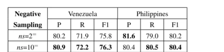
Negative Venezuela Philippines

Sampling P R F1 P R F1

ns=2= _{80.2 71.9 75.8 81.6 79.0 80.2}

ns=10= _{80.9 72.2 76.3 80.4 80.5 80.4}

Table 5 CNN classification results by using word embedding models with different negative sampling sizens={2,10}on both of our datasets.=indicates that the difference betweenns=2 andns=10 is not significant.

sample sizens, we train word embedding models withns={2,10}to cover a value from each range. Since in Section 5.1 word embedding model with context window W =5 and dimensionalityD=500 already attains good performance for the CNN classifiers, we use this setting for all the experiments in this part.

Results on both Venezuela and Philippines datasets are shown in Table 5 by vary-ing the value ofns. A largernsgives slightly better performances on recall and F1 scores across two different datasets as highlighted in Table 5. However, since a larger negative sample size ns requires much more training time,ns=10 does not ben-efit the CNN classifiers much compared to ns=2 in this case. The result of the McNemar’stest also indicates that there is no significant difference between CNN classifiers learned using word embeddings withns=2andns=10. In particular, the word embedding corpora (en-Twitter-general andes-Twitter-general) we used have different size:en-Twitter-generalcontains 12M more tweets and 421K more unique words thanes-Twitter-general. As such we conclude that, a small negative sample size (i.e.ns) is sufficient for our Twitter election classification task.

5.3 Discussion

Compared to the studies on other tasks such as named entity recognition (NER) and dependency parsing (see Section 2), our results differ from their conclusions that “a smaller context window size gives a better performance” [3, 15]. Such a contradiction suggests that the best setup of parameters such as context window and dimensionality may differ from our task to another. For example, both Bansal et al. [3] and Mitra et al. [25] have noted that the learned word embeddings can be type-based or topic-based due to different context window sizes. Bansal et al. [3] clustered two word embeddings that are learned using context window size 1 and 10, respectively. The example clusters showed that, when context window sizeW =1, syntactic words (e.g. his, your, her and its) are close to each other in the embedding space. On the contrary, topical words (e.g. financing, equity, investor and stock) are close to each other in the embedding space learned using context window sizeW =10.

Following the aforementioned work, we study our Spanish Twitter word em-beddings that were learned with dimensionalityD=200 and context window sizes W ={1,5}. Using thecosinesimilarity defined in Eq. (1), we retrieve the most sim-ilar words from the embedding space given a query word. Examples are shown in Table 6 using two query words “futbol (football)” and “venezuela”. We observe that the closest words to “futbol” are mostly the names of football players whenW =1.

W Query Retrieved words

W1 futbol hokey, messi, suarez, #barcelonavsrealmadrid, neymar, ronaldo venezuela #envide, oposicion, #vzlanoesunaamenaz, @ntn24ve, #angelustim, @fholland

W5 futbol lionel, segun, messi, despidieron, banquillo, #barcelonavsrealmadrid venezuela venezue, @delgadoantoniom, #concluvzla, venezeula, vzla, veneuela

Table 6 Example words retrieved usingcosinesimilarity for embeddings with window sizeW=1 and

W=5. Retrieved words are listed in descending order ofcosinesimilarity.

However, forW =5, we note that some topical words are also included such as “de-spidieron (dismiss)” and “banquillo (bench)”. For the query word “venezuela”, the retrieved words are mostly hashtags and Twitter handles for context windowW =1, while some typos and abbreviations (e.g. “veneuela” and “vzla”) of “venezuela” ap-pear in the retrieved words forW=5. This clearly shows that a large context window size (e.g.W =5) allows word embedding models to learn relationships of two words that are more topic-based than a small context window size (e.g.W =1). Therefore, in our examples, the abbreviations and typos of “venezuela” can be related in the embedding space.

Our findings together with the observations from Bansal et al. [3] and Mitra et al. [25] are helpful to explain the contradiction between the results of the NER task [15] and our Twitter election classification task. In the NER task, the classifier aims to identify named entities (e.g. names of persons, organisations and locations), which are often composed of a few adjacent words or the same type of words. There-fore, the word embedding model learned with a small context window benefits the NER task by relating the words having the same type (e.g. relating “futbol” to foot-ball players’ names as shown in Table 6). In our Twitter election classification task, the CNN classifiers aim to classify tweets by the topics within their content. As such, a word embedding model learned with a large context window helps the CNN classi-fiers to capture the semantic information, the typos and even the abbreviations about the same topic.

In summary, for the Twitter election classification task using CNNs, word embed-dings with large context window and dimension size can outperform all our baselines including the state-of-the-art text classifierfastText, in particular, achieving a statis-tically significant improvement over the classic classification baseline of SVM with TF-IDF for the Venezuela dataset. Therefore, we answerRQ1, that for our Twitter election classification task, a large context window size is preferred which is different to that from other tasks (e.g. Dependency parsing [3] and NER [15]).

6 Effect of the background corpora

Due to the noisy nature of Twitter data, Twitter posts can often be poor in grammar and spelling. Meanwhile, Twitter provides more special information such as Twitter handles, HTTP links and hashtags which would not appear in common text corpora. In order to studyRQ2and infer whether the type of background corpus could af-fect the Twitter classification performance, we compare the background corpora of

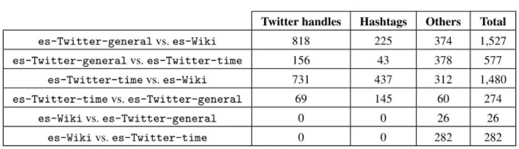
Twitter handles Hashtags Others Total es-Twitter-generalvs.es-Wiki 818 225 374 1,527 es-Twitter-generalvs.es-Twitter-time 156 43 378 577 es-Twitter-timevs.es-Wiki 731 437 312 1,480 es-Twitter-timevs.es-Twitter-general 69 145 60 274 es-Wikivs.es-Twitter-general 0 0 26 26 es-Wikivs.es-Twitter-time 0 0 282 282

Table 7 Statistics of the pair comparison in unique vocabulary of Spanish background corpora (e.g.

es-Twitter-generalvs.es-Wikishows unique words only covered byes-Twitter-general

com-pared toWiki)

es-Wiki,es-Twitter-generalandes-Twitter-timefor Venezuela dataset. We compareen-Wiki,en-Twitter-generalanden-Twitter-timefor Philippines dataset. By considering the various experimental results reported in Section 5, we set the context window to 5 and the dimensionality to 500 for the word embeddings used in this section since they have demonstrated good performance for the CNN classifiers.

6.1 Types of background corpora

Before we show the effect of the types of background corpora, we first compare the word embedding models trained from Wikipedia corpus and Twitter corpus. Take the Spanish word embeddings as an example, the pairwise comparison (Table 7) between

es-Wikiandes-Twitter-generalshows vocabulary difference of the word em-bedding models. As we show the salient statistics of the two background corpora in Table 2, 66% of the vocabulary of our Venezuela election dataset appear in the word embedding model trained fromes-Twitter-generalwhile only 51% appear ines-Wiki. By removing the words shared by both embedding models, we observe that 1,527 unique words are covered byes-Twitter-generalbut not covered by

es-Wikifrom Table 7. However, there are only 26 unique words that are covered byes-Wikionly. In Table 7, es-Twitter-generalvs.es-Wikicategorises the words only found ines-Twitter-general, which are mostly words unique to Twit-ter, such as Twitter handles and hashtags. The other 374 words are mainly incorrect spellings and elongated words such as “bravoooo”, “yaaaa” and “urgenteeeee”, which occur more often in Twitter than in other curated types of data such as Wikipedia. Our initial study on the vocabulary coverage shows that when the type of background cor-pus aligns with our Twitter classification task, it can potentially cover more unique terms that often occur in Twitter.

The classification results are shown in Table 8, where the first column shows the dataset we used. In other columns, we report three measures for embedding models trained from two types of background corporaes-Wikiandes-Twitter-general

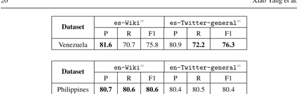
for Venezuela election dataset anden-Wikianden-Twitter-generalfor Philip-pines election dataset. For each dataset, the best scores are highlighted in bold. From Table 8, we observe that when the type of background corpus aligns with our Twitter

Dataset es-Wiki = _{es-Twitter-general}= P R F1 P R F1 Venezuela 81.6 70.7 75.8 80.9 72.2 76.3 Dataset en-Wiki = _{en-Twitter-general}= P R F1 P R F1 Philippines 80.7 80.6 80.6 80.4 80.5 80.4

Table 8 Classification results by using different background corpora on Venezuela and Philippines datasets.=_{indicates that the difference between Wikipedia and Twitter corpus is not significant.}

election datasets, the performance is better for Venezuela dataset in terms of recall and F1 scores. However, the performances of the two word embedding models on Philippines dataset are very similar. As such, we conduct theMcNemar’stest, which indicates that the difference between the two types of word embedding models is not significant when applied to our Twitter election classification task. The additional words learned byes-Twitter-general(as categorised in Table 7) do not signifi-cantly affect the classification performance.

6.2 Time periods of background corpora

We have shown in Section 6.1 there is no significant difference between the two background data types. However, when the type of background corpus aligns with the dataset (e.g. Twitter data), will the covered time period affect the classifica-tion performance? To address this quesclassifica-tion, we first compare the performance of

es-Twitter-generalandes-Twitter-timewhere the latter one covers the elec-tion period of the Venezuela elecelec-tion dataset; similarly, for Philippines dataset, we compareen-Twitter-generalanden-Twitter-time.

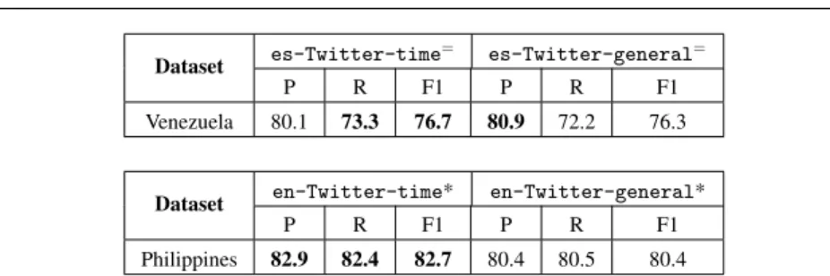
For each dataset, the classification results are shown in Table 9 . For the Venezuela dataset, es-Twitter-time slightly outperforms es-Twitter-general in recall and F1 scores. However, according to McNemar’s test, this difference between the embedding models trained fromes-Twitter-generalandes-Twitter-timeis not statistically significant, with a p-value greater than 0.05. For the Philippines dataset, as shown in Table 9,en-Twitter-timeoutperformsen-Twitter-general

on all the metrics. Moreover, theMcNemar’stest confirms that the performance dif-ference is significant betweenen-Twitter-timeanden-Twitter-general. From Table 2, by comparing the number of tweets collected in both of the corpora of

en-Twitter-generalanden-Twitter-time, we notice that although the corpus

en-Twitter-timehas a fewer number of tweets and unique words after prepro-cessing, it has a similar word coverage on our Philippines election dataset. Thus, it indicates that for our particular classification task a smaller background corpus is capable to capture most of the salient words to distinguish different classes.

Furthermore, from Table 7, we notice that compared toes-Twitter-general,

es-Twitter-timecovers more hashtags but fewer Twitter handles. By investigating the hashtags only covered by thees-Twitter-time, we note that they correspond

Dataset es-Twitter-time

= _{es-Twitter-general}=

P R F1 P R F1

Venezuela 80.1 73.3 76.7 80.9 72.2 76.3

Dataset en-Twitter-time* en-Twitter-general*

P R F1 P R F1

Philippines 82.9 82.4 82.7 80.4 80.5 80.4

Table 9 Classification results of CNN classifiers using word embedding models with and without overlap with the election periods. = _{indicates that the difference between es-Twitter-time and}

es-Twitter-generalis not significant. * indicates the difference betweenen-Twitter-time and

en-Wikiis significant.

to hashtags that were frequently used on Twitter during the 2015 Venezuela parlia-mentary election period, for example “#venezueladecide”, “#vota6d”, “#reporte6d” and “#venezuelacambio”. Since some hashtags are only popular during the election period, by covering the time period of the election datasets, it allows the word embed-ding to provide more domain-based features. In particular, althoughes-Twitter-time

contains fewer number of tweets, it shows comparable classification results on our Twitter election classification task and requires less time for training a word embed-ding compared toes-Twitter-general. For Philippines dataset, by covering the election period, en-Twitter-timeeven outperforms en-Twitter-general sig-nificantly. In summary, in answer toRQ2, we find that aligning both the type and time period of background corpus with the classification dataset leads to better feature representations, and hence a more effective classification using the CNN classifier.

7 Out-of-vocabulary words

Out-of-vocabulary (OOV) words are those that appear in the dataset but not in the word embedding model, and therefore vector representations cannot be obtained for such words. Although a larger background corpus can help word embeddings to cover more words,OOVwords can still appear in Twitter dataset. Indeed, as reported in Ta-ble 2, thees-Twitter-generalcorpus can only cover 66% words in our Venezuela election dataset, for instance due to the occurrence of various hashtags and Twitter handles. In recent studies of word embeddings [6, 18, 25], theOOV words appear in different datasets such as the German dataset, namelyDE-GUR350[34], which is used to study the semantic relatedness of word pairs.OOVwords were simply ignored by Bojanowski et al. [6] and Mitra et al. [25]. On the contrary, Kim [18] randomly ini-tialised the vector representations ofOOVwords by sampling each dimension from a uniform distributionU[−a,a].awas selected in such way that the initialised vectors have the same variance as the learned word embedding model. Since this strategy uses the statistics of the pre-trained word embedding models, we addressRQ3in this section to study whether such kind of strategies improves the classification perfor-mance.

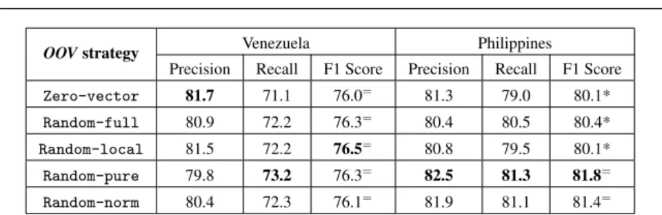
OOVstrategy Venezuela Philippines

Precision Recall F1 Score Precision Recall F1 Score

Zero-vector 81.7 71.1 76.0= _{81.3 79.0 80.1*}

Random-full 80.9 72.2 76.3= _{80.4 80.5 80.4*}

Random-local 81.5 72.2 76.5= _{80.8 79.5 80.1*}

Random-pure 79.8 73.2 76.3= 82.5 81.3 81.8=

Random-norm 80.4 72.3 76.1= _{81.9 81.1 81.4}=

Table 10 Classification results of CNN classifiers by using differentOOVstrategies. Highest score for each dataset is highlighted in bold.=indicates that the difference between each strategy is not significant. * indicates the difference is significant compared toRandom-pure.

We use our word embedding models trained from es-Twitter-general and

en-Twitter-general with the context window size W =5 and dimensionality D=500, since it was already shown in Section 5 to attain good performance. Five different strategies are used in this section:

1. Random-full: Following the strategy used by Kim [18], we randomly initialise theOOVwords using the calculated means and standard deviations from the en-tire pre-trained word embedding model.

2. Random-local: We randomly initialise theOOVwords using the calculated means and standard deviations from only the vector representations of words that appear in the dataset.

3. Zero-vector: We apply a simple strategy similar to the one used by Bojanowski et al. [6] and Mitra et al. [25] to initialise the vector representations ofOOVwords asn-dimensionalzerovectors.

4. Random-pure: We apply a purely random strategy to sample a number from the range(0,1)for each dimension of the vector representations ofOOVwords. 5. Random-norm: We randomly initialise theOOV word using normal distribution

and the means and standard deviations obtained from the word embedding model. An alternative strategy would be the use of a character-based distributed representa-tions approach (e.g. as proposed by Dhingra et al. [11]) to address theOOVproblem. However, in this paper, we omit this approach to focus exclusively on word-level em-bedding models. In particular, character-level approaches (e.g. character-level CNN) cannot reuse pre-trained word-level embedding models, such as those obtained from Twitter or Wikipedia. Therefore, we leave the character-level approaches to future work. The classification performances of the aforementioned retained strategies are compared in Table 10 over precision, recall and F1 scores for Venezuela and Philip-pines datasets.

From Table 10, we observe that indeed all the random initialisation strategies of

Random-full,Random-local,Random-pureandRandom-normslightly improve the attained recall and F1 scores compared to theZero-vectorstrategy – indeed, this conclusion agrees with the observation of Kim [18], who observed slight im-provements using a similar strategy for text classification. However,Zero-vector

strategy has a slightly better precision over random strategies for Venezuela dataset. SinceRandom-localhas the best performance in terms of F1 score for Venezuela

dataset in Table 10, we conduct the statistical test between the two strategies of

Random-localandZero-vector. The result of the statistical test yields ap-value greater than 0.05, which shows that the difference between them is not statistically significant. For the Philippines dataset, we then conduct theMcNemar’stest to com-pareRandom-pureandRandom-norm, since they outperform other strategies. The result of statistical test shows that the difference between the two strategies is not significant with a p-value greater than 0.05. Hence, we conclude that, compared to simple strategies (e.g.Zero-vectorandRandom-pure), a more complicated ran-dom initialisation strategy that uses the means and standard deviations of word em-beddings does not significantly improve the performance of CNN classifiers on both datasets.

In summary, the simplest strategies (e.g.Zero-vectorandRandom-pure) are able to achieve comparable or better classification performance toRandom-normand

Random-full, which shows simple strategies are sufficient for our Twitter election classification task. This answers our RQ3 that there is no obvious preference be-tween the differentOOV strategies studied in this section (e.g.Random-norm and

Random-pure), since their classification performances are comparable according to the statistical test.

8 Conclusions

Since previous investigations on the parameter configuration of word embeddings fo-cus on different tasks such as NER [15] and dependency parsing [3], their findings may not generalise to Twitter classification tasks. Meanwhile, similar work on Twit-ter classification tasks [13, 28, 32] have not studied the impact of background corpora andWord2Vecparameters such as the context window and dimensionality. Our find-ing shows that these two factors can indeed affect the classification performance on Twitter classification tasks. In particular, in this paper, we studied word embeddings when using convolutional neural networks. Using two different types of background corpora, we observed that when the type and time period of background corpus aligns with the classification dataset, the CNN classifier can achieve significantly better per-formance on Twitter data (Section 6). In particular, our investigation showed that choosing the correct type of background corpus can potentially cover more vocabu-lary of the classification dataset. Thus, the alignment between the background corpus and the classification dataset provides better tweet-level representations. For infer-ring the best setup of Word2Vec parameters (e.g. context window, dimensionality and negative samples), we applied word embeddings with various parameter setup to convolutional neural networks (Section 5). As a practical guide for a Twitter clas-sification task, word embeddings with both large context windows and dimension are preferable to attain high effectiveness with a CNN classifier. In contrast, the number of negative samples does not affect the performance of a CNN classifier in our task. In addition, we show that there is no obvious winner among the currentOOVstrategies for our Twitter classification task using CNN classifiers and word embedding models (Section 7). Thus, the simplest random strategy of sampling each dimension of the OOVword vectors from range(0−1)is sufficient to deal with theOOVwords.

Acknowledgements This paper was supported by a grant from the Economic and Social Research Coun-cil, (ES/L016435/1).

References

1. Venezuela opposition politician luis manuel diaz killed. http://www.bbc.co.uk/news/world-latin-america-34929332 (2015). URL http://www.bbc.co.uk/news/

world-latin-america-34929332. [Accessed: 2016-05-15]

2. Amati, G., Amodeo, G., Bianchi, M., Marcone, G., Bordoni, F.U., Gaibisso, C., Gambosi, G., Celi, A., Di Nicola, C., Flammini, M.: FUB, IASI-CNR, UNIVAQ at TREC 2011 microblog track. In: Proc. of TREC (2011)

3. Bansal, M., Gimpel, K., Livescu, K.: Tailoring continuous word representations for dependency pars-ing. In: Proc. of ACL, vol. 2, pp. 809–815 (2014)

4. Bengio, Y., Ducharme, R., Vincent, P., Janvin, C.: A neural probabilistic language model. Journal of machine learning research3, 1137–1155 (2003)

5. Bermingham, A., Smeaton, A.F.: On using Twitter to monitor political sentiment and predict election results. In: Proc. of SAAIP workshop at IJCNLP (2011)

6. Bojanowski, P., Grave, E., Joulin, A., Mikolov, T.: Enriching word vectors with subword information. arXiv preprint arXiv:1607.04606 (2016)

7. Cohen, J.: Weighted kappa: Nominal scale agreement provision for scaled disagreement or partial credit. Psychological bulletin70(4), 213 (1968)

8. Collobert, R., Weston, J.: A unified architecture for natural language processing: Deep neural net-works with multitask learning. In: Proc. of ICML, pp. 160–167 (2008)

9. Collobert, R., Weston, J., Bottou, L., Karlen, M., Kavukcuoglu, K., Kuksa, P.: Natural language pro-cessing (almost) from scratch. Journal of machine learning research12, 2493–2537 (2011) 10. Conneau, A., Schwenk, H., Barrault, L., Lecun, Y.: Very deep convolutional networks for natural

language processing. arXiv preprint arXiv:1606.01781 (2016)

11. Dhingra, B., Zhou, Z., Fitzpatrick, D., Muehl, M., Cohen, W.W.: Tweet2vec: Character-based dis-tributed representations for social media. ACL (2016)

12. Dietterich, T.G.: Approximate statistical tests for comparing supervised classification learning algo-rithms. Neural computation10(7), 1895–1923 (1998)

13. Ebert, S., Vu, N.T., Sch¨utze, H.: CIS-positive: Combining convolutional neural networks and SVMs for sentiment analysis in Twitter. In: Proc. of SemEval, p. 527 (2015)

14. Glorot, X., Bordes, A., Bengio, Y.: Deep sparse rectifier neural networks. In: Proc. of AISTATS, vol. 15, p. 275 (2011)

15. Godin, F., Vandersmissen, B., De Neve, W., Van de Walle, R.: Multimedia Lab@ ACL W-NUT NER shared task: Named entity recognition for Twitter microposts using distributed word representations. In: Proc. of ACL-IJCNLP, p. 146 (2015)

16. Hahnloser, R.H., Sarpeshkar, R., Mahowald, M.A., Douglas, R.J., Seung, H.S.: Digital selection and analogue amplification coexist in a cortex-inspired silicon circuit. Nature405(6789), 947–951 (2000) 17. Joulin, A., Grave, E., Bojanowski, P., Mikolov, T.: Bag of tricks for efficient text classification. arXiv

preprint arXiv:1607.01759 (2016)

18. Kim, Y.: Convolutional neural networks for sentence classification. In: Proc. of EMNLP, pp. 1746– 1751 (2014)

19. Krizhevsky, A., Sutskever, I., Hinton, G.E.: Imagenet classification with deep convolutional neural networks. In: Proc. of NIPS, pp. 1097–1105 (2012)

20. Macdonald, C., McCreadie, R., Santos, R.L., Ounis, I.: From puppy to maturity: Experiences in de-veloping terrier. In: Proc. of OSIR workshop at SIGIR, vol. 60 (2012)

21. Mikolov, T., Chen, K., Corrado, G., Dean, J.: Efficient estimation of word representations in vector space. arXiv preprint arXiv:1301.3781 (2013)

22. Mikolov, T., Le, Q.V., Sutskever, I.: Exploiting similarities among languages for machine translation. arXiv preprint arXiv:1309.4168 (2013)

23. Mikolov, T., Sutskever, I., Chen, K., Corrado, G.S., Dean, J.: Distributed representations of words and phrases and their compositionality. In: Proc. of NIPS, pp. 3111–3119 (2013)

24. Mikolov, T., Yih, W.t., Zweig, G.: Linguistic regularities in continuous space word representations. In: Proc. of HLT-NAACL, vol. 13, pp. 746–751 (2013)

25. Mitra, B., Nalisnick, E., Craswell, N., Caruana, R.: A dual embedding space model for document ranking. arXiv preprint arXiv:1602.01137 (2016)

26. Pedregosa, F., Varoquaux, G., Gramfort, A., Michel, V., Thirion, B., Grisel, O., Blondel, M., Pretten-hofer, P., Weiss, R., Dubourg, V., Vanderplas, J., Passos, A., Cournapeau, D., Brucher, M., Perrot, M., Duchesnay, E.: Scikit-learn: Machine learning in Python. Journal of machine learning research12, 2825–2830 (2011)

27. Pennington, J., Socher, R., Manning, C.D.: Glove: Global vectors for word representation. In: Proc. of EMNLP, pp. 1532–1543 (2014)

28. Severyn, A., Moschitti, A.: UNITN: Training deep convolutional neural network for Twitter sentiment classification. In: Proc. of SemEval, pp. 464–469 (2015)

29. Severyn, A., Nicosia, M., Barlacchi, G., Moschitti, A.: Distributional neural networks for automatic resolution of crossword puzzles. In: Proc. of ACL-IJCNLP (2015)

30. Srivastava, N., Hinton, G.E., Krizhevsky, A., Sutskever, I., Salakhutdinov, R.: Dropout: a simple way to prevent neural networks from overfitting. Journal of Machine Learning Research15(1), 1929–1958 (2014)

31. Tang, D., Qin, B., Liu, T.: Document modeling with gated recurrent neural network for sentiment classification. In: Proc. of EMNLP, pp. 1422–1432 (2015)

32. Tang, D., Wei, F., Yang, N., Zhou, M., Liu, T., Qin, B.: Learning sentiment-specific word embedding for Twitter sentiment classification. In: Proc. of ACL, vol. 1, pp. 1555–1565 (2014)

33. Wang, P., Xu, J., Xu, B., Liu, C.L., Zhang, H., Wang, F., Hao, H.: Semantic clustering and convolu-tional neural network for short text categorization. In: Proc. of ACL-IJCNLP, vol. 2, pp. 352–357 (2015)

34. Zesch, T., Gurevych, I.: Automatically creating datasets for measures of semantic relatedness. In: Proc. of Linguistic Distances workshop at ACL, pp. 16–24 (2006)

35. Zhang, X., LeCun, Y.: Text understanding from scratch. arXiv preprint arXiv:1502.01710 (2015) 36. Zhang, X., Zhao, J., LeCun, Y.: Character-level convolutional networks for text classification. In:

Proc. of NIPS, pp. 649–657 (2015)

37. Zhang, Y., Wallace, B.: A sensitivity analysis of (and practitioners’ guide to) convolutional neural networks for sentence classification. arXiv preprint arXiv:1510.03820 (2015)