c
INFORMATION THEORETIC AND MACHINE LEARNING TECHNIQUES FOR EMERGING GENOMIC DATA ANALYSIS
BY MINJI KIM
DISSERTATION
Submitted in partial fulfillment of the requirements
for the degree of Doctor of Philosophy in Electrical and Computer Engineering in the Graduate College of the
University of Illinois at Urbana-Champaign, 2017
Urbana, Illinois
Doctoral Committee:
Professor Olgica Milenkovic, Co-Chair Professor Jun S. Song, Co-Chair Professor Venugopal V. Veeravalli Professor Saurabh Sinha
ABSTRACT
The completion of the Human Genome Project in 2003 opened a new era for scientists. Through advanced high-throughput sequencing technologies, we now have access to a large amount of genomic data and we can use it to answer key biological questions, such as the factors contributing to the de-velopment of cancer. Large data sets and rapidly advancing sequencing tech-nology pose challenges for processing and storing large volumes of genomic data. Moreover, the analysis of datasets may be both computationally and theoretically challenging because statistical methods have not been devel-oped for new emerging data. In this work, I address some of these problems using tools from information theory and machine learning.
First, I focus on the data processing and storage aspect of metagenomics, the study of microbial communities in environmental samples and human organs. In particular, I introduce MetaCRAM, the first software suite spe-cialized for metagenomic sequencing data processing and compression, and demonstrate that MetaCRAM compresses data to 2-13 percent of the original file size.
Second, I analyze a biological dataset assaying the propensity of a DNA sequence to form a four-stranded structure called “G-quadruplex” (GQ). GQ structures have been proposed to regulate diverse key biological processes including transcription, replication, and translation. I present main factors that lead to GQ formation, and propose highly accurate linear regression and Gaussian process regression models to predict the ability of a DNA sequence to fold into GQ.
Third, I study data structures to analyze and store three-dimensional chro-matin conformation data generated from high-throughput sequencing tech-nologies. In particular, I examine statistical properties of Hi-C contact maps and propose a few suitable formats to encode pairwise interactions between genome locations.
ACKNOWLEDGMENTS
My graduate study was filled with blessings from the following individuals. I must first acknowledge my referees, anonymous reviewers, and the se-lection committee of the NSF Graduate Research Fellowship application for their strong support in funding my study for three years. I also thank Profes-sors Venugopal V. Veeravalli, Saurabh Sinha, Jian Peng, Sua Myong, Doctor Alex Kreig, and members of the Milenkovic and Song group for their valuable feedback and discussions on my work.
My parents deserve ample credit for promoting both my scholarly and mu-sical activities, through which I made life-long friends to emotionally support me. I was also fortunate enough to study with a Hungarian Violinist J´anos N´egyesy, who was the first one to recognize my lack of confidence. As a solution, he told me to think big and play big. Whenever I encountered dis-couraging moments in graduate school, I reminded myself to think big and study big. Thank you for your violin and life lessons, and rest intrue peace, J´anos. Another source of support was Professor Tara Javidi, who strongly encouraged me to pursue doctoral degree. Her recommendation brought me to my current advisor in Illinois.
Professor Olgica Milenkovic welcomed me with interesting problems in bioinformatics, and I thank her for this new direction. Among many qual-ities, I truly admire her creativity and intellectual curiosity. My co-advisor Professor Jun S. Song is also a great role model. I respect his dignity and meticulousness, and thank him for training me. I would like to call them my academic parents, who had higher expectations for me than my biological parents had. Through their investment and belief in my intellectual growth, I finally felt worthy. Thus, I dedicate this humble thesis to my beloved aca-demic parents.
TABLE OF CONTENTS
CHAPTER 1 INTRODUCTION . . . 1
1.1 Introduction to Molecular and Cellular Biology . . . 1
1.2 Genomics . . . 2
1.3 Sequencing Technologies . . . 4
1.4 Thesis Overview . . . 6
CHAPTER 2 METAGENOMIC READ PROCESSING AND COM-PRESSION . . . 8
2.1 Background . . . 8
2.2 Methods . . . 11
2.3 Results . . . 20
2.4 Discussion . . . 28
CHAPTER 3 QUANTITATIVE ANALYSIS AND PREDICTION OF G-QUADRUPLEX FOLDING PROPENSITY . . . 30
3.1 Background . . . 30
3.2 Methods . . . 33
3.3 Results . . . 39
3.4 Discussion . . . 53
CHAPTER 4 DATA STRUCTURES TO ANALYZE AND STORE 3D GENOME MAPS . . . 57 4.1 Background . . . 57 4.2 Methods . . . 60 4.3 Results . . . 65 4.4 Discussion . . . 66 REFERENCES . . . 71
CHAPTER 1
INTRODUCTION
1.1
Introduction to Molecular and Cellular Biology
Before delving into genomics, we first review fundamental concepts in molec-ular and cellmolec-ular biology, summarized from parts of Cooper and Hausman [1]. A well-established cell theory in molecular biology states that: 1) all living organisms are composed of one or more cells, 2) the cell is the most basic unit of life, and 3) all cells arise from pre-existing cells. This theory highlights the importance of studying cells in living organisms.
The information coding for cell functions is contained in deoxyribonucleic acid (DNA). DNA is composed of four nucleotides: cytosine (C), thymine (T), adenine (A), and guanine (G), where C and G form a pair through three hydrogen bonds and A and T form a pair through two hydrogen bonds (Figure 1.1). It is worth noting that an extra hydrogen bond between C and G makes it a stronger pair than A and T. These complementary base pairings allows DNA not only to maintain a double-stranded helical struc-ture but also toreplicate itself. When the double-stranded DNA (dsDNA) is denatured, i.e., hydrogen bonds are broken, an enzyme may use one strand as a template and add complementary pairs. This process, called DNA repli-cation, produces an exact copy of the original dsDNA.
DNA molecules may be copied into another similar macromolecule called ribonucleic acid (RNA). RNA, composed of thymine (T), uracil (U), adenine (A) and guanine (G), lacks a hydroxyl group and is usually single-stranded. The process of copying the DNA to RNA is called transcription.
A triplet of single-stranded RNA codes for one of 20 amino acids. The amino acids ultimately build proteins, which perform major functions in our cells. This ultimate process of converting RNA to protein is calledtranslation. The central dogma of molecular biology, encompassing replication,
transcrip-Figure 1.1: Complementary base pairing of right-handed double helical DNA strands. Adenine and thymine are paired through two hydrogen bonds, and cytosine and guanine are paired by three hydrogen bonds. Major grooves are wider than minor grooves. Illustration by Zephyris (Own work) [CC BY-SA 3.0 or GFDL], via Wikimedia Commons.
tion, and translation, is crucial in understanding cell functions (Figure 1.2).
1.2
Genomics
In Section 1.1, we learned that cells’ functions are largely governed by protein, but the information itself is encoded in the DNA. Thus, we must first look at the genome of an organism, the DNA content in the cell. For example, the human genome consists of approximately 3 billion DNA base pairs and has been identified in the early 2000s.
Genomics is the study of genomes. A sequence of DNA encodes a specific protein through transcription and translation, but the functions of each part of the genome have not been fully understood. Furthermore, the amount of protein is often controlled by unknown external factors. One of the goals of genomics is to catalog functional elements of the genome and to understand how the genome is organized to fulfill these functions.
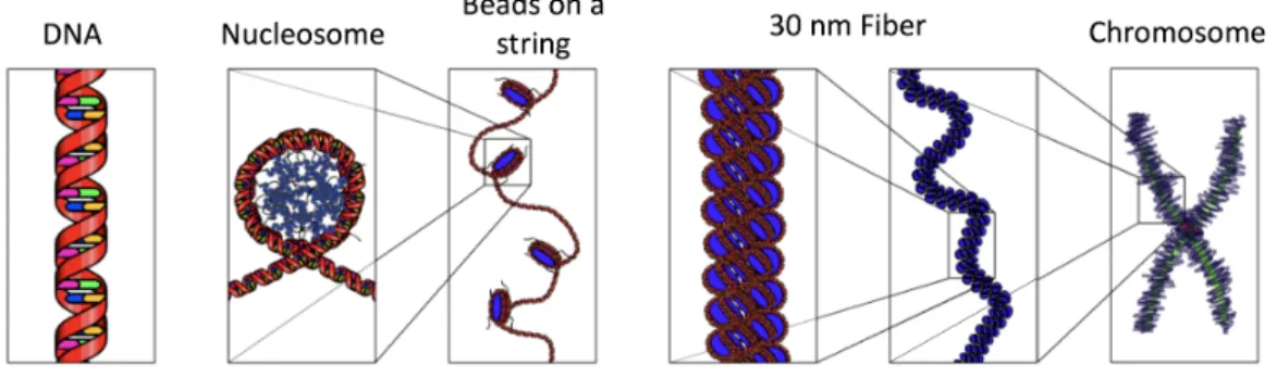
Storing all 3 billion base pairs in a small cell requires efficient hierarchi-cal structures (Figure 1.3). The naked DNA strands are first coiled and
Figure 1.2: Central dogma of molecular biology: a flow from DNA to
protein. DNA polymerase replicates the DNA, RNA polymerase transcribes the DNA to RNA, and the ribosome translates RNA to protein products. Illustration by Central Dogma of Molecular Biochemistry with
Enzymes.jpg: Dhorspool derivative work:Miguelferig [CC BY-SA 3.0], via Wikimedia Commons.
wrapped around positively charged histone core proteins and form nucleo-somes, which look like the “beads” on a string of DNA strands. Addition of the linker histone H1 further compresses to the 30 nm fibers and finally forms a chromosome. The center of the chromosome is called the centromere, and the telomere at the end protects the chromosome.
The central dogma explained in this section relies on the accessibility of machineries to the naked DNA. Both replication and transcription require the addition of complementary nucleotide bases to the template strand. Con-sequently, parts of the tightly packed genomes have to be unwound for repli-cation and transcription. Epigenomics is a subarea of genomics in which the goal is to understand the mechanisms behind chromatin structures and modifications and their roles in gene regulations. We will revisit this concept in Chapter 4.
Figure 1.3: Hierarchical organization of chromatin structures. A double-helical DNA is wrapped around histone proteins to form a
nucleosome. The sequence of more than one nucleosome resembles beads on a string, and is further compressed into 30 nm fiber. Chromosome
represents the most condensed form of our genome. Illustration by Richard Wheeler at en.wikipedia [GFDL or CC-BY-SA-3.0], from Wikimedia
Commons.
1.3
Sequencing Technologies
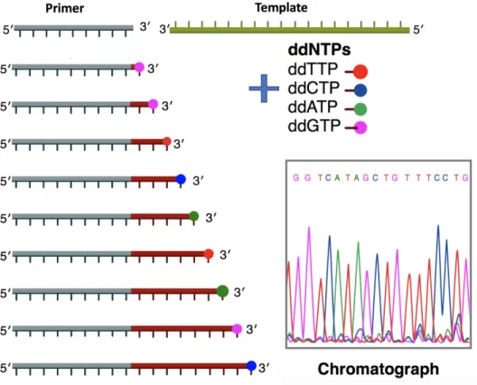
Sequencing refers to the precise reading of the genome. One of the earliest techniques, Sanger sequencing, is the chain-termination method developed by Frederick Sanger in the 1970s (Figure 1.4). Here, each of the four dideoxynu-cleotides (dNTPs) ddTTP, ddCTP, ddATP, and ddGTP is labeled with red, blue, green and pink fluorescent dye, respectively, and indicates the randomly terminated position of the genome. As a result, we obtain the genome by reading the colors at each position. The Sanger method is accurate, but the process is often laborious especially if we want to sequence a large genome.
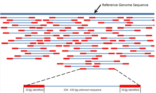
There have been improvements to the Sanger and related methods, but a major breakthrough in molecular biology occurred with the invention of high-throughput (formerly next-generation) sequencing. Because it is difficult to read long genomes at once, the technique fragments the genome into smaller pieces. Combined with an amplification step via a polymerase chain reac-tion (PCR), we obtain many short segments of the genome called the reads. Moreover, paired-end sequencing has been developed to increase the accu-racy: a single short read may have come from multiple parts of the genome, but if another pair further away is sequenced, we can identify the precise location by requiring that both pairs have to match the reference genome. In Figure 1.5, the reads are placed such that the sequences of red parts overlap.
Figure 1.4: The Sanger method for DNA sequencing. Each of the four dideoxynucleotides ddTTP, ddCTP, ddATP, ddGTP is labeled with red, blue, green and pink fluorescence dye to indicate nucleotide base at a terminating location. With the primer, DNA template, DNA polymerase and dNTPs in mixture, the primer elongates and the chain terminates. By reading the population of labeled strands, we obtain a chromatograph and recover the genome sequence. Illustration by Estevezj (Own work) [CC BY-SA 3.0], via Wikimedia Commons.
and many algorithms have been developed to accurately assemble a genome. High-throughput sequencing technique has been applied to diverse domains in genomics. For example, it can sequence the DNA (whole genome se-quencing) and RNA (RNA-seq), target parts of DNA occupied by a specific protein (ChIP-seq), identify modified parts of the chromatin (WGBS), find open chromatin regions (DNase-seq and ATAC-seq), and most recently, ob-tain genome-wide contact maps (5C, Hi-C, and ChIA-PET). Some of these domains are explored in subsequent chapters.
Figure 1.5: High-throughput paired-end sequencing method. Short regions in red are sequenced from both ends and they are jointly mapped to the reference genome shown in blue. In case the genome has not been sequenced, the overlapping reads can be assembled into a genome. Illustration by Suspencewl (Own work) [CC0], via Wikimedia Commons
1.4
Thesis Overview
As seen in the previous section, advanced high-throughput sequencing tech-nologies allow us to access a large amount of genomic data and we can use it to study cancer, evolution, development, and much more. Unfortunately, we face the challenge of processing and storing a large volume of genomic data because sequencing technologies are advancing at a faster rate than computation capabilities. Moreover, the analysis of a large dataset may be both computationally and theoretically challenging because statistical meth-ods have not been developed for new emerging data. In this work, I address some of these problems using tools from information theory and machine learning.
First, I focus on the data processing and storage aspect of the problem. Due to the low cost of sequencing today, at about $1000 to sequence a human genome, researchers generate a massive amount of data. We currently store more than 100 petabytes of sequencing data, and by 2025 we are projected to have 2-40 exabytes of data [2]. There are several options to mitigate this problem. One option is to discard the data after the project has been
completed. However, some biological data may not be easily reproducible, and we may need the data in the future for a related project. A simple solution is to buy more hard drives, but 40 exabytes of hard disks would be extremely costly. The last option, which is pursued by scientists and engineers, is to compress the data.
Data compression, also known as source coding, is a subfield of information and coding theory in which various dictionary-based (Lempel-Ziv) to entropy-based (Huffman) methods have been developed. These encoding algorithms have been widely adopted to compress general text files, such as in gzip and bzip. However, these general tools are not suitable for compressing genomic data because we can get a better rate by exploiting certain properties of a particular dataset. Previously, compression tools for FASTA, FASTQ, and BAM/SAM files have been developed, but no known algorithm existed for metagenomic data. Thus, I present a statistical and information theoretical approach to compress metagenomic reads.
Second, I analyze biological data to extract meaningful information by using regression methods, which are widely used in the machine learning community. Regression analysis is a statistical process for estimating the relationships among variables, and it is different from a classification problem in that we focus on continuous outcome rather than discrete classes. In particular, I use linear regression and Gaussian process regression methods to predict the ability of a DNA sequence to fold into a secondary structure called “G-quadruplex”.
Last, I propose several data formats to store 3D genome contact maps. Recent technologies such as Hi-C, ChIA-PET, and their variants provide pairwise genome interactions information. The data are generally stored as a two-dimensional matrix, but a long genome at a fine resolution produces an extremely large matrix. We can exploit statistical properties of the contact maps, such as symmetry and sparsity in some cases, to efficiently store large data. A natural extension of this work would be to compress the data of the optimal format.
The thesis is organized as follows: in Chapter 2, I present MetaCRAM, a compression tool for metagenomic sequencing reads; in Chapter 3, the regression models are designed to predict G-quadruplex forming sequences with high accuracy; and I propose 3D genome data formats in Chapter 4.
CHAPTER 2
METAGENOMIC READ PROCESSING
AND COMPRESSION
2.1
Background
2.1.1
Introduction to Metagenomics
Metagenomics is an emerging discipline focused on genomic studies of com-plex microorganismal population. In particular, metagenomics enables a range of analyses pertaining to species composition, the properties of the species and their genes as well as their influence on the host organism or the environment. As the interactions between microbial populations and their hosts plays an important role in the development and functionality of the host, metagenomics is becoming an increasingly important research area in biology, environmental and medical sciences. As an example, the National In-stitute of Health (NIH) recently initiated a far-reaching Human Microbiome Project [3] which has the aim to identify species living at different sites of the human body (in particular, the gut and skin[4]), observe their roles in regulating metabolism and digestion, and evaluate their influence on the im-mune system. The findings of such studies may have important impacts on our understanding of the influence of microbials on an individual’s health and disease, and hence aid in developing personalized medicine approaches. Another example is the Sorcerer II Global Ocean Sampling Expedition [5], led by the Craig Venter Institute, the purpose of which is to study microor-ganisms that live in the ocean and influence/maintain the fragile equilibrium of this ecosystem.
There are many challenges in metagenomic data analysis. Unlike classical genomic samples, metagenomic samples comprise many diverse organisms, the majority of which is usually unknown. Furthermore, due to low sequenc-ing depth, most widely used assembly methods – in particular, those based
on de Bruijn graphs – often fail to produce quality results and it remains a challenge to develop accurate and sensitive meta-assemblers. These and other issues are further exacerbated by the very large file size of the samples and their ever increasing number. Nevertheless, many algorithmic methods have been developed to facilitate some aspects of microbial population analysis: examples include MEGAN (MEta Genome ANalyzer) [6], a widely used tool that allows for an integrative analysis of metagenomic, metatranscriptomic, metaproteomic, and rRNA data; and PICRUSt (Phylogenetic Investigation of Communities by Reconstruction of Unobserved States) [7], developed to predict metagenome functional contents from 16S rRNA marker gene se-quences. Although suitable for taxonomic and functional analysis of data, neither MEGAN nor PICRUSt involve a data compression component, as is to be expected from highly specialized analytic software.
2.1.2
Literature review on genomic data compression
In parallel, a wide range of software solutions have been developed to ef-ficiently compress classical genomic data (a comprehensive survey of the state-of-the-art techniques may be found in [8]). Specialized methods for compressing whole genomes have been reported in [9, 10, 11], building upon methods such as modified Lempel-Ziv encoding and the Burrows-Wheeler transform. Compression of reads is achieved by mapping the reads to refer-ence genomes and encoding only the differrefer-ences between the referrefer-ence and the read; or, in a de novo fashion that does not rely on references and uses classical sequence compression methods. Quip [12] and CRAM [13] are two of the best known reference-based compression algorithms, whereas ReCoil [14], SCALCE [15], MFCompress [16], and the NCBI Sequence Read Archive method compress data without the use of reference genomes. Reference-based algorithms in general achieve better compression ratios than reference-free al-gorithms by exploiting the similarity between some predetermined reference and the newly sequenced reads. Unfortunately, none of the current reference-based method can be successfully applied to metagenomic data, due to the inherent lack of “good” or known reference genomes. Hence, the only means for compressing metagenomic FASTA and FASTQ files is through the use of de novo compression methods.
2.1.3
Highlights of MetaCRAM
As a solution to the metagenomic big data problem, we introduce MetaCRAM, the firstde novo, parallel, CRAM-like software specialized for FASTA-format metagenomic read compression, which in addition provides taxonomy iden-tification, alignment and assembly information. This information primarily facilitates compression, but also allows for fast searching of the data in the compressive domain and for basic metagenomic analysis. The gist of the classification method is to use a taxonomy identification tool – in this case, Kraken [17] – which can accurately identify a sufficiently large number of organisms from a metagenomic mix. By aligning the reads to the identified reference genomes of organisms via Bowtie2 [18], one can perform efficient lossless reference-based compression via the CRAM suite. Those reads not aligned to any of the references can be assembled into contigs through exist-ing metagenome assembly software algorithms, such as Velvet [19] or IDBA-UD [20]; sufficiently long contigs can subsequently be used to identify addi-tional references through BLAST (Basic Local Alignment Search Tool) [21]. The reads aligned to references are compressed into the standard CRAM format [13], using three different integer encoding methods, Huffman [22], Golomb [23], and Extended Golomb encoding [24].
MetaCRAM is an automated software with many options that accommo-date different user preferences, and it is compatible with the standard CRAM and SAMtools data format. In addition, its default operational mode is loss-less, although additional savings are possible if one opts for discarding read ID information. We report on both the lossless and “lossy” techniques in the Methods Section. MetaCRAM also separates the read compression pro-cess from the quality score compression technique, as the former technique is by now well understood while the latter is subject to constant changes due to different quality score formats in sequencing technologies. These changes may be attributed to increasing qualities of reads and changes in the cor-relations of the score values which depend on the sequencing platform. For quality score compression, the recommended method is QualComp [25].
MetaCRAM offers significant compression ratio improvements when pared to standard bzip and gzip methods, and methods that directly com-press raw reads. These improvements range from 2-4-fold file size reduc-tions, which leads to large storage cost reductions. Furthermore, although
MetaCRAM has a relatively long compression phase, decompression may be performed in a matter of minutes. This makes the method suitable for both real time and archival applications.
2.2
Methods
2.2.1
Algorithmic overview
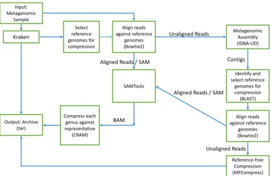
The block diagram of the MetaCRAM algorithm is given in Figure 2.1, and the operation of the algorithm may be succinctly explained as follows. The first step is to identify suitable references for compression, which is achieved by identifying dominant taxonomies in the sample. The number of references is chosen based on cut-off abundance thresholds, which themselves are chosen using several criteria that trade-off compression ratio and compression time. Once the references are chosen, the raw reads are aligned to their closest references and the starting positions of the reads are statistically analyzed to determine the best integer compression method to be used for their encod-ing. Furthermore, reads that do not align sufficiently well with any of the chosen references are assembled using IDBA UD, and the contig outputs of the assembler are used to identify additional references via BLAST search. Reads not matched with any references after multiple iterations of the above procedure are compressed independently with the MFCompress suite. The results associated with each of the described processing stages are discussed in the next subsections. Note that here and throughout the paper, we use standard terms in genomics and bioinformatics without explanations.
2.2.2
Pre-processing
MetaCRAM accepts both unpaired and paired-end reads. If paired-end reads are given as an input to MetaCRAM, then the first preprocessing step is to append the read IDs with a “ 1” or a “ 2” indicating that the read came from the first or second mate, respectively. Another preprocessing step includes filtering out the quality scores in case that the input file is in FASTQ format. This filtering process allows for using new and emerging quality score com-pression methods without constantly updating the MetaCRAM platform.
Note that the paired end labeling is done automatically, while filtering can be implemented outside the integrated pipeline by the user, based on his/her requirements for quality score lossy or lossless compression goals.
MetaCRAM uses as a default FASTA files that do not contain quality val-ues, in which case the resulting SAM file contains the symbol “I” repeated as many times as the length of the sequence. These symbols amount to about 100 bytes per read, and this overhead increases proportionally to the number of reads. In order to reduce the size of this unnecessary field, MetaCRAM replaces the sequence of “I”s with a single symbol “*”, complying with the standard SAM format. Likewise, read IDs are highly repetitive in nature: for instance, every read ID starts with the data name such as “SRR359032.”, followed by its unique read number. Rather than repeating the data name for every read, we simply store it once, and append it when performing decom-pression. Both versions of MetaCRAM – one incorporating these two options – and another one without the described features are available to the user. The former version of the methods requires a slightly longer compression and decompression time.
2.2.3
Taxonomy identification
Given the labeled read sequences of a metagenomic sample, the first step is to identify the mixture of species present in the sample. There are sev-eral taxonomy identification methods currently in use: the authors of [26] proposes to use the 16S rRNA regions for bacterial genome identification, MetaPhyler [27] scans for unique markers exceeding length 20 and provides a taxonomy level as specific as the genus. On the other hand, a new taxon-omy identification software known as Kraken [17], based on exact alignment of k-mers to the database of known species, often outperforms MetaPhyler and other methods both in terms of speed and discovery of true positives, as indicated by our tests.
MetaCRAM employs Kraken as a default tool in the pipeline. Kraken produces an output report which is automatically processed by MetaCRAM. Part of the report contains information about species present in the sam-ple, as well as their abundance. We rank order the species from the most abundant to the least abundant, where abundance is based on the number of
reads identified to match a species in the database. For downstream analysis, MetaCRAM selects the “most relevant” species and uses their genomes as references. The default definition of “most relevant” is the top 75 species, but one has the option to choose a threshold for the abundance value or for the number of references used. As an illustration, Table 2.2 (p. 22) lists the results of an analysis of the impact of different thresholds on the processing time and the compression ratio.
2.2.4
Alignment and assembly
After a group of reference genomes is carefully chosen based on the Kraken software output, alignment of reads to the reference genomes is performed. This task is accomplished by using Bowtie2 [18], a standard software tool for ultra-fast alignment of short reads to long genomes. The alignment in-formation is stored in a SAM (Sequence Alignment/Map) file format and subsequently used for compression via reference-based algorithms.
Due to the fact that many species in a metagenome sample have never been sequenced before, some reads will not be aligned to any of the references, and we collectively refer to them asunaligned reads hereafter. In order to discover reference genomes for unaligned reads, we assemble the unaligned reads using a metagenomic assembler. Our metagenomic assembler of choice is IDBA-UD [20], given that in our tests it produced the largest number of contigs leading to new reference identification. Alternatives to IDBA-UD include the Ray Meta software [28].
When the reads have high sequencing depth and large overlaps, thecontigs produced by the assembler may be queried using BLAST [21] to identify the organisms they most likely originated from. The user may choose to BLAST only the top n longest contigs, where n is a user specified number, but in our analysis we use all contigs. Subsequently, we align the unaligned reads to the newly found references.
2.2.5
Distribution of read starting positions
We empirically studied the distribution of integers representing the read po-sitions, variation popo-sitions, and paired-end offsets in order to choose the most
Kraken Select reference genomes for compression Align reads against reference genomes (Bowtie2) Metagenomic Assembly (IDBA-UD) Identify and select reference genomes for compression (BLAST) Align reads against reference genomes (Bowtie2) SAMTools Compress each genus against representative (CRAM) Reference-free Compression (MFCompress) Output: Archive (tar) Unaligned Reads Unaligned Reads Aligned Reads / SAM
Aligned Reads / SAM Contigs
Input: Metagenomic
Sample
BAM
Figure 2.1: The block diagram of the MetaCRAM Algorithm for
Metagenomic Data Processing and Compression. Its main components are taxonomy identification, alignment, assembly and compression.
suitable compression method. As an example, the distribution of the start-ing positions for the reads that aligned to JH603150 (genome of Klebsiella oxytoca) in the dataset SRR359032 is shown in Figure 2.2. This distribution was truncated after achieving a 90% coverage of the data (i.e., after only 10% of the read start positions exceeded the depicted maximum length). The em-pirical distribution is shown in yellow, while a fitted power law distributions is plotted and determined according to [24], with Pi = 2−logmi2i(m1−1), where i is the integer to be encoded, and m is the divisor in the extended Golomb code. The chosen parameters are m = 3 and 4. The negative binomial dis-tribution is fitted using Maximum Likelihood Estimation (MLE), while the geometric distribution is fitted by two different means: using MLE and ezfit, a MATLAB script that performs an unconstrained nonlinear minimization of the sum of squared residuals with respect to various parameters.
For single reference alignment methods, it was reported that the best fit for the empirical distribution is a geometric distribution or a negative bino-mial distribution [29]. However, due to sequencing errors and non-uniform distributions of hydrogen bond breakage (also referred as the “GC bias”), the empirical data often deviates from geometric and negative binomial
dis-tributions [30]. In addition, for metagenomic samples, there exist multiple references which may have good alignments with reads that did not originally correspond to the genomic sample of the reference. This creates additional changes in the read starting position with respect to the geometric distri-bution. Moreover, one has to encode not only the read positions but also the variation positions and paired-end offsets, making it difficult to claim any one of the fitted distributions is better than others. This observation is supported by Figure 2.2. Since there is no known efficient optimal encoding method for a set of integers with negative binomial distributions, and Golomb and extended Golomb encoding are optimal for geometric distributions and power law distributions, respectively, we use these two methods withm = 3. The parameter m is chosen based on extensive experiments, although the user has the freedom to adjust and modify its value.
Figure 2.2: Integer Distribution. Distribution fitting of integers to be encoded, truncated at 90% of the integer data.
As the number of unaligned reads that remains after a few iterations of MetaCRAM is relatively small, these reads were compressed using a reference-free tool such as MFCompress [16], which is based on finite-context models. Furthermore, the SAM files produced after running Bowtie2 are converted to the sorted and indexed binary format of a BAM file using SAMtools [31]. Each BAM file is compressed via reference-based compression against its rep-resentative to a standard CRAM format. We tested three different modes of the CRAM toolkit [13]: Huffman, Golomb, and Extended Golomb encoding,
all of which are described in the next section. Note that the Extended Golomb encoding method is our new addition to the classical CRAM method, as it appears to offer good compromises between compression and decompression speed and compression ratios.
Intrinsically, SAM files contain quality values and unique read IDs for each read, which inevitably account for a large file size: quality values are characters of length as long as the sequence, and read IDs often repeat the name of the dataset. By default, MetaCRAM preserves all quality values and read IDs as designed in CRAM.
2.2.6
Compression
Compression in the reference-based mode is accomplished by compressing the starting points of references with respect to the reference genomes and the base differences between the reads and references. As both the starting points and bases belong to a finite integer alphabet, we used three different integer compression methods, briefly described below.
Huffman coding is a prefix-free variable length compression method for known distributions [22] which is information-theoretically optimal [32]. The idea is to encode more frequent symbols with fewer bits than non-frequent ones. For example, given an alphabetA= (a, b, c, d, e) and the corresponding distribution P = (0.25,0.25,0.2,0.15,0.15), building a Huffman tree results in the codebook C = (00,10,11,010,011) (Figure 2.3). Decoding relies on the Huffman tree constructed during encoding which is stored in an efficient manner, usually ordered according to the frequency of the symbol. Due to the prefix-free property, Huffman coding is uniquely decodable and does not require any special marker between words. Two drawbacks of Huffman cod-ing are its storage complexity, since we need to record large tree structures for big alphabet size, and the need to know the underlying distribution a priori. Adaptive Huffman coding mitigates the second problem, at the cost of increased computational complexity associated with constructing multiple encoding trees [33]. In order to alleviate computational challenges, we imple-mented so called canonical Huffman encoding, which bypasses the problem of storing a large code tree by sequentially encoding lengths of the codes [34]. Golomb codes are optimal prefix-free codes for countably infinite lists of
Figure 2.3: Huffman tree constructed for an alphabet A= (a, b, c, d, e) with distribution P = (0.25,0.25,0.2,0.15,0.15).
non-negative integers following a geometric distribution [23]. In Golomb coding, one encodes an integer n in two parts, using its quotient q and remainder r with respect to the divisor m. The quotient is encoded in unary, while the remainder is encoded via truncated binary encoding. Given a list of integers following a geometric distribution with known mean µ, the dividend m can be optimized to reduce code length. In [35], the optimal value of m was derived for m = 2k, for any integer k. The encoding is
known as the Golomb-Rice procedure, and it proceeds as follows: first, we let k∗ =max ( 0,1 + log2 log(φ−1) log µµ+1 ) , where φ = ( √ 5+1) 2 . Unary coding
represents an integer i through runs of i ones followed by a single zero. For example, the integer i = 4 in unary is 11110. Truncated binary encoding is a prefix-free code for an alphabet of size m, which is more efficient than standard binary encoding. Because the remainder r can only take values in {0,1,. . . , m-1}, according to truncated binary encoding, we assign to the first 2k+1−m symbols codewords of fixed length k. The remaining symbols are
encoded via codewords of length k+ 1, where k =blog2(m)c. For instance, given n = 7 and m = 3, we have 7 = 2×3 + 1, implying q = 2 and r = 1. Encoding 2 in unary gives 110 and 1 in truncated binary reads as 10. Hence, the codeword used to encode the initial integer is the concatenation of the two representations, namely 11010.
Decoding of Golomb encoded codewords is also decoupled into decoding of the quotient and the remainder. Given a codeword, the number of ones before the first zero determines the quotientq, while the remainingkork+ 1 bits, represents the remainder r according to truncated binary decoding for an alphabet of size m. The integer n is obtained as n=q×m+r.
Golomb encoding is computationally more efficient than Huffman cod-ing because it only requires division operations. Furthermore, one does not need to the distribution a priori, although there are clearly no guarantees that Golomb coding for an unknown distribution will be even near-optimal: Golomb encoding is optimal only for integers following a geometric distribu-tion.
An extension of Golomb encoding, termed extended Golomb [24] coding, is an iterative method for encoding non-negative integers following a power law distribution. One divides an integer n by m until the quotient becomes 0, and then encodes the number of iterations M in unary, and an array of remaindersr according to an encoding table. This method has an advantage over Golomb coding when encoding large integers, such is the case for read position compression. As an example, consider the integer n = 1000: with
m = 2, Golomb coding would produce q= 500 and r= 0, and unary encod-ing of 500 requires 501 bits. With extended Golomb codencod-ing, the number of iterations equals M = 9 and encoding requires only 10 bits. As an illustra-tion, let us encode n = 7 given m = 3. In the first iteration, 7 = 2×3 + 1, so r1 = 1 is encoded as 10, and q1 = 2. Since the quotient is not 0, we
iterate the process: 2 = 0×3 + 2 implies r2 = 2, which is encoded as 1, and
q2 = 0. Because the quotient is at this step 0, we encode M = 2 as 110 and
r =r2r1 = 110, and our codeword is 110110.
The decoding of extended Golomb code is also performed in M iterations. Since we have a remainder stored at each iteration and the last quotient
qM = 0, it is possible to reconstruct the original integer. Similar to Golomb
coding, extended Golomb encoding is computationally efficient, but optimal only for integers with power law distributions.
There are various other methods for integer encoding, such as Elias Gamma and Delta Encoding [36], which are not pursued in this paper because they do not appear to offer good performance for the empirical distributions observed in our read position encoding experiments.
2.2.7
Products
The compressed unaligned reads, CRAM files, list of reference genomes (op-tional), alignment rate (op(op-tional), contig files (optional) are all packaged
into an archive. The resulting archive can be stored in a distributed manner and when desired, the reads can be losslessly reconstructed via the CRAM toolkit.
2.2.8
Decompression
Lossless reconstruction of the reads from the compressed archive is done in two steps. For those reads with known references in CRAM format, decom-pression is performed with an appropriate integer decomdecom-pression algorithm. When the files are converted back into the SAM format, we retrieve only the two necessary fields for FASTA format, i.e., the read IDs and the se-quences printed in separate lines. Unaligned reads are decompressed sepa-rately, through the decoding methods used in MFCompress.
2.2.9
Post-processing
The two parts of reads are now combined into one file, and they are sorted by the read IDs in an ascending order. If the reads were paired-end, they are separated into two files according to the mate “flag” assigned in the pre-processing step.
2.2.10
Effects of parallelization
One key innovation in the implementation of MetaCRAM is parallelization of the process, which was inspired by parallel single genome assembly used in TIGER [37]. Given that metagenomic assembly is computationally highly demanding, and in order to fully utilize the computing power of a standard desktop, MetaCRAM performs meta assembly of unaligned reads and com-pression of aligned reads in parallel. As shown in Table 2.1, parallelization improves real, user, and system time by 23 – 40 %.
2.2.11
Test datasets
The datasets supporting the results of this article are available in the National Center for Biotechnology Information Sequence Read Archive repository,
un-Table 2.1: Processing time improvements for two rounds of MetaCRAM on the SRR359032 dataset (5.4GB, without removing redundancy in
description lines) resulting from parallelization of assembly and compression.
Time Without Parallelization With Parallelization Reduction (% )
Real 235m 40s 170m 4s 27.7
User 449m 40s 346m 33s 22.9
System 14m 13s 8m 45s 40.1
der accession numbers ERR321482 (http://www.ncbi.nlm.nih.gov/sra/
ERX294615), SRR359032 (http://www.ncbi.nlm.nih.gov/sra/SRX103579),
ERR532393 (http://www.ncbi.nlm.nih.gov/sra/ERX497596), SRR1450398
(http://www.ncbi.nlm.nih.gov/sra/SRX621521), SRR062462 (http://www.
ncbi.nlm.nih.gov/sra/SRX024927).
2.3
Results
We tested MetaCRAM as a stand-alone platform and compared it to MF-Compress, a recently developed software suite specialized for FASTA files, and bzip2 and gzip [38], standard general purpose compression tools (avail-able at http://www.bzip.org). Other software tools for compression of sequencing data such as SCALCE and Quip, and SAMZIP [39] and Slim-Gene [40], were not tested because they were either for FASTQ or SAM file formats, and not FASTA files.
As already pointed out, MetaCRAM does not directly process FASTQ file formats for multiple reasons: 1) the quality of sequencers are improving significantly, reaching the point where quality scores may contain very little information actually used during analysis; 2) reads with low quality scores are usually discarded and not included in metagenomics analysis – only high quality sequences are kept; 3) there exist software tools such as QualComp [25], specifically designed for compressing quality scores that users can run independently along with MetaCRAM.
2.3.1
Taxonomy identification and reference genome selection
As the first step of our analysis, we compared two metagenomic taxonomy identification programs, Kraken and MetaPhyler in terms of computation time and identification accuracy on synthetic data, as it is impossible to test the accuracy of taxonomy identification on real biological datasets. For this purpose, we created mixtures of reads from 15 species, listed in the Additional File 4. The two Illumina paired-end read files were created by MetaSim [41] with 1% error rate, and they amounted to a file of size 6.7 GB. Kraken finished its processing task in 22 minutes and successfully identified all species within the top 50 most abundant taxons. On the other hand, MetaPhyler ran for 182 minutes and failed to identify Acetobacterium woodii and Haloterrigena turkmenica at the genus level. This example illustrates a general trend in our comparative findings, and we therefore adopted Kraken as a default taxonomy retrieval tool for MetaCRAM.
When deciding how to choose references for compression, one of the key questions is to decide which outputs of the Kraken taxonomy identification tool are relevant. Recall that Kraken reports the species identified according to the number of reads matched to their genomes. The most logical approach to this problem is hence to choose a threshold for the abundance values of reads representing different bacterial species, and only use sequences of species with high abundance as compression references. Unfortunately, the choice for the optimal threshold value is unclear and it may differ from one dataset to another; at the same time, the threshold is a key parameter that determines the overall compression ratio – choosing too few references may lead to poor compression due to the lack of quality alignments, while choosing too many references may reduce the compression ratio due to the existence of many pointers to the reference files. In addition, if we allow too many references, we sacrifice computation time for the same final alignment rate. It is therefore important to test the impact of the threshold choice on the resulting number of selected reference genomes.
In Table 2.2, we listed our comparison results for all five datasets studied, using two threshold values: 75 (high) and 10 (low). For these two choices, the results are colored gray and white, respectively. We observe that we get slightly worse compression ratios if we select too few references, as may be seen for the files ERR321482 and ERR532393. Still, the processing time is
significantly smaller when using fewer references, leading to 30 to 80 minutes of savings in real time. It is worth to point out that this result may also be due to the different qualities of internal hard drives: for example, the columns in gray were obtained running the code on Seagate Barracuda ST3000, while the results listed in white were obtained via testing on Western Digital NAS. Table 2.2: Analysis of the influence of different threshold values on
reference genome selection after taxonomy identification and compression ratios. Columns colored in gray represent a threshold of 75 species, while the columns not colored in gray correspond to a cutoff of 10 species. The results are shown for MetaCRAM-Huffman, with original and compressed file sizes in MB and processing time in minutes. “Aln. %” refers to the alignment rates for the first and second round, and “No. files” refers to the number of reference genome files selected in the first and second iteration.
Data Ori. (MB) Com. (MB) Time (min) Aln. % No. files Com. (MB) Time (min) Aln. % No. files ERR321482 1429 191 299m 27 3.6 211 1480 193 239m 24.2 6.5 29 1567 SRR359032 3981 319 127m 57.7 9.7 26 30 320 93m 57.7 9.7 7 32 ERR532393 8230 948 639m 45.8 2 267 1456 963 522m 42.5 7.2 39 1639 SRR1450398 5399 703 440m 7.1 0.6 190 793 703 364m 6.8 0.9 26 818 SRR062462 6478 137 217m 2.6 0.1 278 570 139 197m 2.1 0.5 50 656
Many of the most abundant references may be from the same genus, and this may potentially lead to the problem of multiple alignment due to sub-species redundancy. The almost negligible effect of the number of reference genomes on alignment rate implies that combining them to remove the re-dundancy would improve computational efficiency, as suggested in [42]. Nev-ertheless, extensive computer simulations reveal that the loss due to multiple alignment is negligible whenever we choose up to 75-100 references. There-fore, our recommendation is to use, as a rule of thumb, the threshold 75 in order to achieve the best possible compression ratio and at the same time provide a more complete list of genomic references for further analysis.
2.3.2
Compression performance analysis
Our comparison criteria include the compression ratio (i.e., the ratio of the uncompressed file and the compressed file size), as well as the compression and decompression time, as measured on an affordable general purpose com-puting platform: Intel Core i5-3470 CPU at 3.2 GHz, with a 16 GB RAM. We present test results for five datasets: ERR321482, SRR359032, ERR532393, SRR1450398, and SRR062462, including metagenomic samples as diverse as a human gut microbiome or a Richmond Mine biofilm sample, retrieved from the NCBI Sequence Read Archive [43].
The comparison results of compression ratios among six software suites are given in Table 2.3 and Figure 2.4. The methods compared include three different modes of MetaCRAM, termed Huffman, Golomb and Extended Golomb MetaCRAM.
The result indicates that MetaCRAM using Huffman integer encoding method improves compression ratios of the classical gzip algorithm 2−3-fold on average. For example, MetaCRAM reduces the file size of SRR062462 to only 2% of the original file size. Notably, the users have the options to retrieve the alignment rate, list of reference genomes, contig files, and align-ment information in SAM format. This list may be stored with very small storage overhead and then used for quick identification of files based on their taxonomic content, which allows for selection in the compressive domain.
In the listed results, the column named “Qual Value (MB)” provides the estimated size of the quality scores for each file, after alignment to references found by Kraken. In our implementation, we replaced these scores with a single “*” symbol per read and also removed the redundancy in read IDs. The result shows that these two options provide better ratios than the default ratio, as shown in Table 2.3 column “MCH2”. However, since read IDs may be needed for analysis of some dataset, we also report results for the default “MCH1” mode which does not dispose of ID tags.
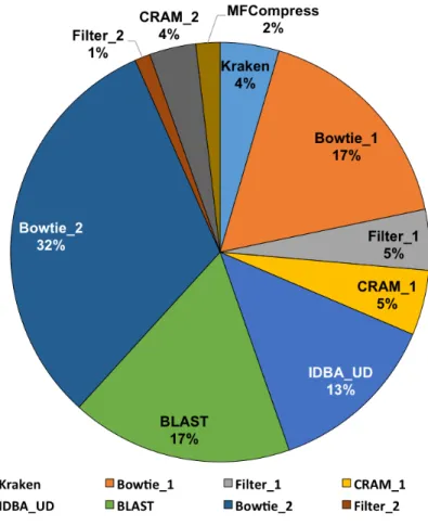
In terms of the processing time shown in Table 2.4 and Figure 2.5, the MetaCRAM suite is at a clear disadvantage, with processing time 150-fold slower than bzip2 in the worst case. Figure 2.6 presents the average run-time of each stage for all five datasets tested, and illustrates that assembly, alignment, and BLAST search are computationally demanding, accounting for 62 percentage of the total time. This implies that removing the second
Table 2.3: Comparison of compression ratios of six software suites. For short hand notation, we used“MCH” = MetaCRAM-Huffman, “MCG” = MetaCRAM-Golomb, “MCEG” = MetaCRAM-extended Golomb,
“MFComp” = MFCompress. “Align. %” refers to the total alignment rates from the first and second iteration. Minimum compressed file size
achievable by the methods are written in bold case letters.
Data Original (MB) MCH (MB) MCG (MB) MCEG (MB) Align. % bzip2 (MB) gzip (MB) MFComp (MB) ERR321482 1429 191 312 213 29.6 362 408 229 SRR359032 3981 319 657 458 61.8 998 1133 263 ERR532393 8230 948 1503 1145 46.8 2083 2366 1126 SRR1450398 5399 703 854 729 7.7 1345 1532 726 SRR062462 6478 137 188 144 2.7 222 356 161
Figure 2.4: The compression ratios for all six software suites, indicating the compression ratio = compressed file sizeoriginal file size .
and subsequent assembly rounds of MetaCRAM reduces the processing time significantly, at the cost of a smaller compression ratio. Table 2.5 compares the compression ratios of MetaCRAM with one round and with two rounds of reference discovery, and indicates that removing the assembly, alignment and BLAST steps adds 1 to 6 MB to the compressed file size. Thus, the user has an option to skip the second round in order to expedite the processing
time.
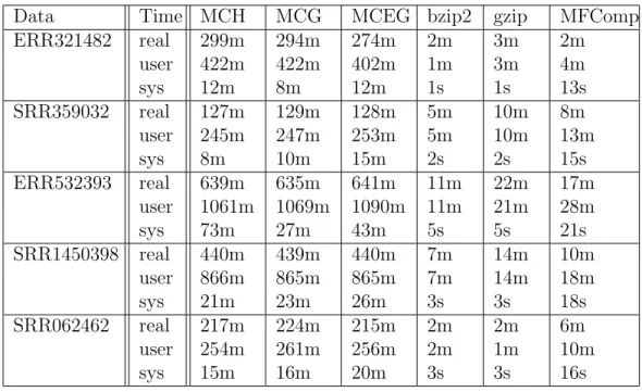
Table 2.4: Comparison of processing (compression) times of six software suites. Times are recorded row by row denoting real, user, and system time in order.
Data Time MCH MCG MCEG bzip2 gzip MFComp
ERR321482 real user sys 299m 422m 12m 294m 422m 8m 274m 402m 12m 2m 1m 1s 3m 3m 1s 2m 4m 13s SRR359032 real user sys 127m 245m 8m 129m 247m 10m 128m 253m 15m 5m 5m 2s 10m 10m 2s 8m 13m 15s ERR532393 real user sys 639m 1061m 73m 635m 1069m 27m 641m 1090m 43m 11m 11m 5s 22m 21m 5s 17m 28m 21s SRR1450398 real user sys 440m 866m 21m 439m 865m 23m 440m 865m 26m 7m 7m 3s 14m 14m 3s 10m 18m 18s SRR062462 real user sys 217m 254m 15m 224m 261m 16m 215m 256m 20m 2m 2m 3s 2m 1m 3s 6m 10m 16s
Figure 2.5: The compression times for all six software suites shown in minutes.
Likewise, Table 2.6 and Figure 2.7 illustrates that the retrieval time of MetaCRAM is longer than that of bzip2, gzip, and MFCompress, but still
Figure 2.6: Average Runtime of Each Stage of MetaCRAM. Detailed distribution of the average runtimes of MetaCRAM for all five datasets tested. We used “ 1” to indicate the processes executed in the first round, and “ 2” to denote the processes executed in the second round.
highly efficient. In practice, the processing time is not as relevant as the retrieval time, as compression is performed once while retrieval is performed multiple times. For long term archival of data, MetaCRAM is clearly the algorithm of choice since the compression ratio is the most important criteria. We also remark on the impact of different integer encoding methods on the compression ratio. Huffman, Golomb, and extended Golomb codes all have their advantages and disadvantages. For the tested datasets, Huffman clearly achieves the best ratio, as it represents the optimal compression method, whereas Golomb and Extended Golomb compression slightly improve com-pression time. However, the parallel implementation of MetaCRAM makes the comparison of processing time of the three methods slightly biased: for example, if we perform compression while performing assembly, compression
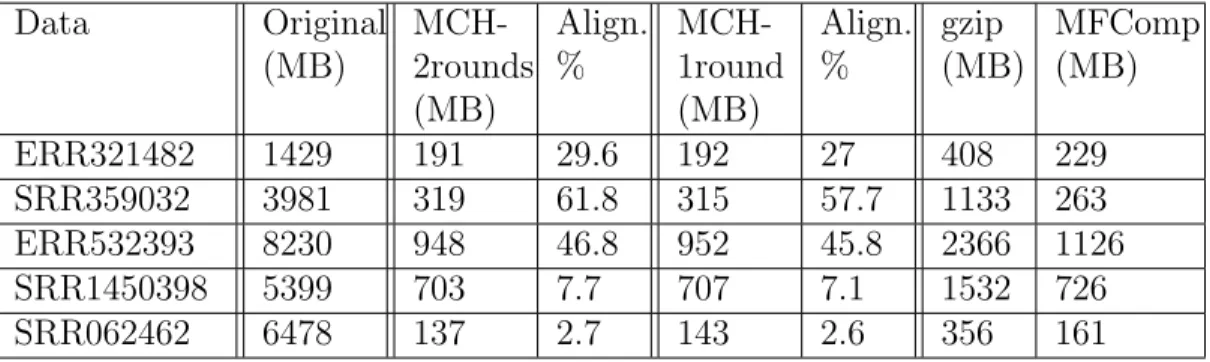
Table 2.5: Comparison of compressed file sizes of MetaCRAM-Huffman using 2 rounds and 1 round. For short hand notation, we
used“MCH-2rounds” = MetaCRAM-Huffman with 2 rounds,
“MCH-1round” = MetaCRAM-Huffman with 1 round. We also used the shortcut “MFComp” = MFCompress and “Align. %” refers to the
percentage of reads aligned during 2 rounds and 1 round, respectively, for MCH-2rounds and MCH-1round.
Data Original (MB) MCH-2rounds (MB) Align. % MCH-1round (MB) Align. % gzip (MB) MFComp (MB) ERR321482 1429 191 29.6 192 27 408 229 SRR359032 3981 319 61.8 315 57.7 1133 263 ERR532393 8230 948 46.8 952 45.8 2366 1126 SRR1450398 5399 703 7.7 707 7.1 1532 726 SRR062462 6478 137 2.7 143 2.6 356 161
Table 2.6: Comparison of retrieval (decompression) times of six software suites. Times are recorded row by row denoting real, user, and system time in order.
Data Time MCH MCG MCEG bzip2 gzip MFComp
ERR321482 real user sys 23m 16m 9m 25m 16m 10m 24m 17m 10m 57s 45s 2s 17s 9s 1s 2m 4m 4s SRR359032 real user sys 12m 11m 2m 11m 11m 1m 13m 12m 3m 2m 2m 4s 1m 28s 2s 8m 15m 19s ERR532393 real user sys 48m 39m 15m 47m 40m 13m 56m 43m 29m 5m 4m 7s 2m 55s 5s 15m 29m 17s SRR1450398 real user sys 28m 30m 7m 28m 29m 5m 29m 30m 7m 3m 3m 5s 2m 37s 3s 10m 19m 26s SRR062462 real user sys 23m 21m 4m 22m 21m 4m 26m 22m 10m 1m 42s 4s 1m 22s 3s 6m 10m 26s
Figure 2.7: The decompression times for all six software suites. will take much more time than compressing while running an alignment al-gorithm. As the processing and retrieval time is not consistent among the three methods, we recommend using Huffman coding for archival storage.
2.4
Discussion
In what follows, we comment on a number of useful properties of the MetaCRAM program, including compatibility, losslessness, partial assembly results and compressive computing.
Compatibility. MetaCRAM uses well established and widely tested
ge-nomic analysis tools, and it also follows the standard gege-nomic data com-pression format CRAM, hence making the results of downstream analysis compatible with a current standard for genomic compression.
Lossless compression principle. By its very nature, MetaCRAM is
a lossless compression scheme as it encodes the differential information be-tween the reference and the metagenomic reads in a 100% accurate fashion. Nevertheless, we enabled a feature that allow for some partial loss of infor-mation, such as the read ID tags. It is left to the discretion of the user to choose suitable options.
CRAM versus MFCompress. MFCompress achieves good compression
achieves a rate proportional to the alignment rate because it only encodes the small difference between the reference genome and the read. As more microbial genome become available, MetaCRAM will most likely offer higher compression ratio than other tools in general. Note that only on one data file - SRR359032 - did MFCompress achieve better compression ratios than MetaCRAM, most likely due to the redundancy issues previously mentioned.
Metagenomic assembly. Metagenomic assembly is a challenging task,
and there is a widely accepted belief that it is frequently impossible to per-form meaningful assembly on mixture genomes containing species from re-lated genomes. Nevertheless, we are using assembly mostly as a means for identifications, but at the same time its output provides useful contigs for gene transfer analysis and discovery. In the case that assembly fails on a dataset, we suggest skipping the assembly step so as to trade off computa-tion time with discovery of new reference genomes and contigs.
Compressive computing. There has been an effort towards
comput-ing in the compressed domain, in order to eliminate the need for persistne compression and decompression time when all one needs to perform is sim-ple alignment [44]. Similarly, MetaCRAM offers easy retrieval and selection based on the list of references stored as an option. For example, suppose we perform MetaCRAM on all available human gut metagenome data. If we want to analyze the datasets with a concentration ofEscherichia coli, we avoid sacrificing retrieval time by quickly scanning the list of reference files and only retrieving the datasets with E. coli.
CHAPTER 3
QUANTITATIVE ANALYSIS AND
PREDICTION OF G-QUADRUPLEX
FOLDING PROPENSITY
3.1
Background
The G-quadruplex (GQ) is a non-canonical DNA secondary structure arising from two or more stacked sets of four guanine (G) nucleotides (G-tetrads) interacting in a plane (Figure 3.1A), although three G-tetrads comprise the most common form in which the four sets of guanine triplets form a four-stranded structure through Hoogsteen base pairing coordinated by monova-lent cations. GQ DNA can assume various folding configurations including parallel, antiparallel, and hybrid conformations dictated by ion conditions and loop sequence compositions [45, 46, 47, 48]. A surge of interest in the GQ structure has followed the recent findings, suggesting its multifaceted role in key processes within the central dogma of biology [49, 50, 51, 52, 53, 54, 55]. In particular, it is hypothesized that the formation of GQs modulates gene expression through a physical interaction between the GQ structure and transcription-related protein complexes [56]. In support, recent work has confirmed the capability of GQs to form stably within the genome [57, 58]. Thus, GQs may prove to be an important component in the regulation of specific genes and, as such, may serve as an effective pharmaceutical target for a wide range of diseases [59, 60, 61, 62]. Putative GQ forming sequences are unevenly distributed throughout the human genome, with their presence increased in select gene regulatory regions, such as promoters of oncogenes and immunoglobulin switch regions [63, 64]. This irregular distribution high-lights the challenge in identifying functional sequences that can actually form GQ structures in vivo.
GQ forming sequences are frequently modeled following the pattern:
GGGNL1GGGNL2GGGNL3GGG, whereN can be adenine (A), cytosine (C),
lengths of the intervening sequences that correspond to loops in the folded GQ structure (Figure 3.1A). We note that loops can contain G bases, al-though we do not consider this possibility in our current study. Typical upper limits on loop length have been suggested to be between 7 and 9 bases within a single-stranded DNA (ssDNA) context, but a maximal loop length has not yet been established in a double-stranded DNA (dsDNA) context [65, 66, 67, 68]. Even with such restricted pattern assumptions, de-termining how nucleotide content and intervening loop lengths control the GQ formation potential of more than 400,000 candidate genomic sequences remains a challenging task. This ambiguity in GQ characterization compli-cates the identification of true GQ forming sequences implicated in essential biological activities.
The discovery of stable genomic GQ formation coupled with the significant number of potential GQ sequences located within the human genome under-scores the need for new tools that can accurately predict folding propen-sity. Owing to the seemingly regular pattern found in GQ forming se-quences, many bioinformatics studies have been conducted on putative GQ sequences [69, 70, 71, 72]. Generally, these studies simply searched for recur-ring patterns of putative GQs or developed models describing folding propen-sity based on GQ experiments in ssDNA. As a result, the methods may be biased towards known patterns and miss novel GQ folding sequences. Previ-ously, we showed that the GQ folding propensity is substantially diminished in dsDNA and that, unlike ssDNA, dsDNA has limited ability to form only into parallel GQs [73]. These considerations highlight the need for a new model that can predict GQ folding propensity specifically in a dsDNA con-text, which is more representative of genomic DNA than ssDNA.
We performed a survey of systematically designed GQ forming sequences to identify folding propensity within a dsDNA context. The survey con-tained more than 400 putative GQ forming sequences with loops composed entirely of A, C, or T with total loop length ranging up to 12 bp. Quan-titative measurement of parallel GQ formation was obtained by N-methyl mesoporphyrin IX (NMM) fluorescence assay that was established in our previous work [73]. The NMM intensity measurements were complemented by single-molecule fluorescence resonance energy transfer (smFRET) exper-iments, which enabled direct quantitation of molecules comprising both the GQ-folded and unfolded populations (Figure 3.1B). We utilized these
com-plementary methods to categorize each sequence as one of “strongly folding”, “non-folding”, or “combined” classes, providing a simple metric for compar-ing the foldcompar-ing propensities of specific putative GQ sequences. Furthermore, by analyzing the impact of loop lengths and compositions on the NMM inten-sity measurement, we identified GQ-driving loop parameters. These results were combined in regression models that can predict GQ folding propensity with high accuracy. Our GQ folding experimental platform and computa-tional models will serve as a useful reference that facilitates the investigation of potential genomic GQs in the future.
G G G L1 L3 L2 N NN N O O O O + NMM Dark Fluorescent P G G G G G G GGG-NL1-GGG-NL2-GGG-NL3-GGG
A
B
C
Non-folding Folding CombinedFigure 3.1: An overview of G-quadruplex structure and the NMM technique. A) A schematic of a parallel GQ structure is depicted. The guanine-guanine Hoogsteen base pairing between each guanine triplet is shown for the sequence GGGNL1GGGNL2GGGNL3GGG, where N denotes
the nucleotide component and L1,L2,L3 are the three loop lengths. B) GQ folding propensity is investigated through an induced fluorescence based assay. The molecule NMM shows a specific increase in fluorescence signal upon binding to a parallel GQ sequence. C) A plate is filled with strong folding sequences in high intensity, combined folding and non-folding sequences in a lower intensity, and non-folding sequences in low intensity.
3.2
Methods
3.2.1
Experimental data
For a given sequence, three readings of NMM measurements were recorded and the average intensity value was used throughout the analysis. We rep-resented the loop components of a GQ sequence using the length vector (L1,L2,L3) and nucleotide content N. For instance, (4,1,2) and N = A
encodes the sequence GGGAAAAGGGAGGGAAGGG. We only considered the cases where all nucleotides in the loops are the same, in order to fully characterize the rules governing these simple, yet poorly understood cases. The total length of intervening sequences is denoted as L =L1 +L2 +L3. We considered combinations of L1, L2, and L3 such that L≤ 12, and N is allowed to be A, C or T. For each N, there are 4 sequences corresponding to
L1 = L2 =L3 and 26×3 sequences corresponding to the case where exactly two of the lengths are equal, accounting for 4 + 26×3 = 82 total points in which at least two of the intervening sequences are repeated. There are a total of 138 possible combinations of loop lengths, such that L1,L2, andL3 are distinct and L ≤12, but we subsampled 64 cases for our measurements in order to reduce the dimension, as explained in Table 3.1. Thus, we have a total of (82 + 64)×3 = 438 readings, corresponding to 146 combinations of loop lengths for three different nucleotides.
We fitted the histogram of intensity values to a mixture of two or three Gaussian distributions by using the Expectation-Maximization algorithm (“mixtools” package in R) and plotted individual values using the “color-Ramps” and “calibrate” packages in R. Categorical histograms based on the nucleotide composition or the minimum loop length composition were plot-ted, and the distribution of a given subset of categories was compared to the rest of the categories via the one-sided unpaired Wilcoxon rank sum test. Finally, we applied the two-sided Kolmogorov-Smirnov test to compare the distributions of T, C, and A pairwise.
3.2.2
Linear regression
As a first step, we na¨ıvely applied a linear regression model of the NMM intensity against the predictor variables L1, L2, L3, seqT, seqC and an
in-Table 3.1: List of all possible data points with unique L1, L2, andL3, such that L1 +L2 +L3≤12, in the ascending order of minL, medL, and maxL without any redundancy in permutation. The test data comprise all 6 permutations of 10 rows highlighted in gray, along with (3,4,5), (5,3,4), (4,3,5), and (4,5,3), summing to data points for each of N =A, C, T.
No. MinL MedL MaxL No. MinL MedL MaxL
1 1 2 3 13 1 4 5 2 1 2 4 14 1 4 6 3 1 2 5 15 1 4 7 4 1 2 6 16 1 5 6 5 1 2 7 17 2 3 4 6 1 2 8 18 2 3 5 7 1 2 9 19 2 3 6 8 1 3 4 20 2 3 7 9 1 3 5 21 2 4 5 10 1 3 6 22 2 4 6 11 1 3 7 23 3 4 5 12 1 3 8
tercept term, where seqT and seqC are indicator variables for T and C nucleotides, respectively. Note that seqA was omitted due to the linear con-straint seqA = 1−seqC −seqT. We then examined an alternative model by replacing L1, L2, L3 with minL, medL, maxL, where minL, medL, and
maxLcorrespond to the minimum, median, and maximum of the three loop lengths. We trained both models on all 438 sequences’ NMM intensities to obtain interpretable coefficients and model prediction. This analysis showed that the second model outperformed the first approach, and we thus used the predictor variables minL, medL, and maxL thereafter. Subsequently, we performed six-fold cross-validation to demonstrate that our model is ro-bust. We randomly partitioned the population into 6 groups, each containing 73 points. Using one group as test data and the remaining five groups as training data, we computed the average coefficient of determination for both test and training data. We adopted the following definition of the coefficient of determination: R2 = 1− Pni=1(yi−yˆi)2
Pn
i=1(yi−y¯)2, where ˆyi is the predicted value and ¯
y= n1Pn
i=1yi is the mean ofnsamples used for calculatingR2. For example, n = 365 for training data, andn= 73 for test data. Likewise, the residual for each sample i is defined as y −yˆ, i.e., the difference between the observed
and predicted values. The linear regression method has many advantages such as its simplicity and the interpretability of the coefficients. However, it has the limitation of assuming linearity of the response in predictor variables.
3.2.3
Gaussian process regression
Gaussian process regression (GPR) is a flexible non-parametric regression method that does not assume linearity of the response in predictor vari-ables [74]. A Gaussian processf is defined on a set X by specifying that the values off on any finite number of points inXform random variables follow-ing a joint Gaussian distribution, with mean 0 and fixed covariance k(x, x0) at x, x0 ∈ X. Thus, we only need to define the covariance function k(x, x0) in order to specify a Gaussian process; k(x, x0) is a kernel that measures the similarity between inputs x and x0. The choice of covariance function plays an important role in model prediction, and a popular choice is the squared exponential function: kSE(x, x0) = σf2e
−(x−x0)2
2l2 +σ2
nδ(x, x
0), where the
hy-perparameters σ2
f and σn2 are the variance of the process and experimental
measurement, respectively, l is the length scale of fluctuation, and δ(x, x0) is the Kronecker delta function. Forntraining data points (xi, yi),i= 1, . . . , n,
we construct an n byn covariance matrix
K = k(x1, x1) k(x1, x2) . . . k(x1, xn) k(x2, x1) k(x2, x2) . . . k(x2, xn) .. . ... . .. ... k(xn, x1) k(xn, x2) . . . k(xn, xn) .
For a test data point x∗, we define
K∗ =
h
k(x∗, x1) k(x∗, x2) . . . k(x∗, xn)
i
and K∗∗ =k(x∗, x∗). Then, the joint distribution of the observed output y
and predicted output y∗ is assumed to be
" y y∗ # ∼N " 0 0 # , " K K∗T K∗ K∗∗ #! ,
and the predictive distribution isy∗|y∼N(K∗K−1y, K∗∗−K∗K−1K∗T). We
subsequently obtain our prediction as the mean ¯y∗ = K∗K−1y. The above
methods were all implemented using GPML MATLAB package [75].
Choice of covariance functions. A valid covariance function k(x, x0)
requires the function to be symmetric and positive semi-definite. In addition, many of the widely used kernels are stationary, i.e., it is a function of only the distance r = |x−x0|. Two examples of stationary covariance functions are a noiseless squared exponential kSE(r) = e−
r2
2l2, with length-scale param-eter l, and a Mat´ern class kM at,v(r) = 2
1−ν Γ(ν) √ 2νr l ν Kν √ 2νr l , with positive parameters ν and l, and a modified Bessel function of the second kind Kν.
For half-integer ν, the Mat´ern function Kν is a product of an exponentially
decaying function and a polynomial, withν = 12 giving a non-smooth process. Asν → ∞, the Mat´ern function behaves similarly to the squared exponential function, which is smooth. We used parameters of different length for each predictor variable, adding flexibility to the input space.
Denoting our predictors (minL, medL, maxL, seqA, seqC, seqT) as (x1, x2, x3, x4, x5, x6), we defined our noiseless covariance function as
k((x1, . . . , x6),(x01, . . . , x 0 6)) = x4x04σ 2 f,AkM at,ν=5/2((x1, x2, x3),(x01, x 0 2, x 0 3)) + x5x05σf,C2 kSE((x1, x2, x3),(x01, x 0 2, x 0 3)) + x6x06σ 2 f,TkM at,ν=3/2((x1, x2, x3),(x01, x 0 2, x 0 3)),
where kM at,ν() is the Mat´ern kernel with specific ν, kSE() is the squared
exponential kernel, and σ2
f,A, σf,C2 , σf,T2 correspond to the variance of the
process for seqA, seqC, and seqT, respectively. This combination has been derived by testing the squared exponential and Mat´ern class withν = 12,32,52
separately for seqA, seqC, seqT, and choosing the best function for each nucleotide.
Estimation of hyperparameters. There are four hyperparameters
σf,N, l1,N, l2,N, l3,N (the length scale for minL, medL, maxL, respectively)
for each nucleotide N, summing to 12. A common method to estimate a set of hyperparameters θ is by maximizing the marginal log-likelihood logp(y|X, θ) = −1 2y TK−1 y y− 1 2log|Ky| − n 2 log(2π), where Ky = K +σ 2 nI
also adopted this method, but implemented it in two steps. First, for each individual nucleotide, we initialized each of l1,N, l2,N, l3,N and σf,N to be 5,
and obtained an estimate by using a conjugate gradient method. Note that there are three separate estimates for σf,N, obtained for each of l1,N, l2,N,
and l3,N, and that we let the final estimate be the average of the three. We
then initialized all 12 hyperparameters with the values obtained from the previous step and maximized the marginal log-likelihood over all lengths and nucleotides. This approach allows for more flexibility in each length scale than treating each loop length with an equal weight. Finally, we estimated
σn2 = 18 as the empirical covariance of our replicate experimental NMM in-tensity measurements. Table 3.2 contains the estimated hyperparameters