UDC 336.76
JEL Classification: C22, C53, G11, G17 DOI: 10.17223/19988648/49/12
E.S. Lavrenova, T.G. Ilina
A NOTE ON THE PREDICTABILITY OF THE RUSSIAN STOCK MARKET
Over the past 20 years, the problem of low investment activity of private investors has been featuring the Russian stock market. There are various reasons for that, among them the financial crises, limited access to information, a high subjectivity and lack of developed and simple methods for making investment decisions. Therefore, this re-search aims to study the predictability of the Russian stock market in the conditions of instability due to crises, as well as the limited access of private investors to infor-mation and the low investment literacy in general. This research addresses the pre-dictability of the equity premium on the Russian stock market from 31 January 2008 to 31 January 2017. This is the period of two economic crises for the Russian econo-my: from 2008 to 2013 and from 2014 to 2017. The authors investigate whether the returns of industry portfolios can predict future stock market returns. The particular set of traditional macroeconomic variables functioning as predictors of stock returns and the economy, in general, is determined. Thus, the selection of approaches, meth-ods, and indicators for the analysis and forecasting of the Russian stock market was carried out according to three criteria: the instability (crises) periods, the information available for the private investor (generally accepted indicators), and the clarity and ordinariness of analysis and forecasting methods. A macroeconomic indicator-based approach or an industry-based approach is more often used for these purposes. Tak-ing into account the instability caused by the economic crises in Russia, the authors combined two approaches. Using traditional linear regression modeling, three out of nine industries and five out of eight macroeconomic predictors have been found sta-tistically significant. However, all the models based on these predictors have negative pseudo-R-squared values; therefore, they underperform the historical out-of-sample mean model. It has also been revealed that two out of nine forecast models, based on significant predictors, provide utility gains for the mean-variance investor.
Keywords: equity premium, Russian stock market, stock prediction, macroeconomic variables, industry indices.
Introduction
Over the past decade, the Russian stock market has been developing under the conditions of globalization causing an increase in the internationalization of securities markets and competition in international financial markets. However, the Russian financial market is still not competitive on the global market.
The problem of low investment activity of private investors has been featur-ing the Russian stock market. There are various reasons for that, among them the financial crises, limited access to information, a high subjectivity and lack of developed and simple methods for making investment decisions [1, р. 8].
There-fore, this research aims to study the predictability of the Russian stock market in conditions of instability due to crises, as well as the limited access of private investors to information and the low investment literacy in general.
In order to maintain and stimulate economic growth in Russia, it is necessary to provide a well-developed financial center. Today, the Russian stock market is not sufficiently developed. The national stock market has limited capacity, in-sufficient to ensure investment needs of Russian companies. It lags behind the world’s largest and most developed equity markets. Further development of the Russian stock market will ensure a balanced, innovation-based, and stable eco-nomic growth in Russia in the long run.
According to analysts, the Russian stock market is expected to further de-cline. The almost complete absence of the collective investment schemes, as well as the low investment attractiveness as a whole, is among the factors of the weakness of the Russian equity capital market.
Successful prediction of the future equity premium could lead to obtaining considerable returns. For the purpose of forecasting future market changes and making an investment decision, investors tend to take into account the historical price performance. The stock returns predictability represents a widely studied subject in the economic literature. There are various points of view on forecast-ing the performance of the stock market. For instance, an efficient market hy-pothesis assumes that stock prices reflect the currently available information, and all changes in prices are not dependent on the recently obtained information. Hence, movements of market prices cannot be predicted in general. According to an opposing view, there are different methods that allow generating infor-mation about future market prices. The equity premium predictability problem and forecasting methods for stock market movements still remain open and con-troversial.
The main objective of this paper is to study various approaches to predicting stock market returns and to create relevant forecast models reflecting movement of the Russian stock market for the private investor.
The study consists of two parts: theoretical and empirical. Part I of our study focuses on the theoretical and empirical review of publications on our research issues. Besides, a brief overview of the Russian stock market, the study data-base, and methodology are presented. An empirical analysis is performed using econometric methods. Finally, results are outlined and compared to those avail-able from previous studies; conclusions are drawn.
In Part II, the empirical model is mainly based on the linear regression analy-sis. For the purpose of this study, the initial database is analyzed over two peri-ods. First, we apply in-sample (full sample) performance evaluation. We use traditional predictive regressionmodeling, which accounts for industry and other macroeconomic indicators and market returns. Second, we conduct out-sample performance evaluation. We divide the total sample into the following two peri-ods: from t to t1, and from t1 to t2. In the beginning, we estimate the model, using data from the t-to-t1 period, and then we reiterate this procedure in rela-tion to the most predictable industries and indicators, using the last three
ob-served years as the out-of-sample period. In the end, we compute forecast errors as a discrepancy between the real values of the out-of-sample period and the forecasting measures. We determine whether the derived model is a better per-formance predictor than the model based on historical returns.
At the final stage of our empirical calculations, we estimate the mean-variance investor’s utility gains and decide whether it will be profitable for him to use the equity premium predictions derived from the models to make invest-ment decisions. We calculate the difference between the average utility for the investor, whose investment decisions are based on the predictive model, and the average utility for the investor, who formed portfolio using only information about the historical mean returns for the out-of-sample period (net average bene-fit).
Literature review
The selection of approaches, methods, and indicators for analyzing and fore-casting of the Russian stock market was carried out according to three criteria: the instability (crises) periods, the information available for the private investor (generally accepted indicators), and the clarity and ordinariness of analysis and forecasting methods.
Predicting stock returns is extremely important for the solution of many fun-damental economic and financial issues. Therefore, it is logical that researchers spend time and resources trying to find economic indicators capable of predict-ing stock returns.
For the purpose of this paper, we have studied numerous articles related to equity premium prediction. There are various methods for performing this anal-ysis. The most widespread approach is predictive linear regression, which re-veals dependence between stock market returns and some market indicators, such as inflation, dividend yield, or default spread. Most publications on predict-ing stock returns confirm a linear relation between market indices and stock re-turns, i.e., it is possible to predict future stock market movements applying econometric approaches.
Several authors showed that, despite a number of econometric problems, it is possible to obtain a considerable predictive component from in-sample studies [3, 4]. Other authors suppose that the future stock price is unpredictable [5, 6, 7].
Regarding the Russian stock market, most of the authors conclude that the impact of oil prices on the Russian stock market performance is weak and not regular and not significant after 2006 [8].
Many authors also prove the dependence of the Russian stock market on for-eign exchanges, such as the U.S. or Germany [9].
The empirical model is mainly based on the analysis of Hong et al. [10]. Us-ing GLS estimator, they test whether the returns of the 34 U.S. industry indices forecast stock market movements.
Thus, the selection of approaches, methods, and indicators for analyzing and forecasting of the Russian stock market was carried out according to three
criteria: the instability (crises) periods, the information available for the private investor (generally accepted indicators), and the clarity and ordinariness of analysis and forecasting methods. A macroeconomic indicator-based approach or an industry-based approach is more often used for these purposes. Taking into account the instability in Russia caused by the economic crises, we combined two approaches to estimate models based on the industry portfolios and a particular set of traditional macroeconomic variables.
A brief overview of the Russian stock market
Today, the Russian stock market is emerging and has a lot of problems that prevent further progress of the market.
The history of the Russian stock market began in 1993 when the main regu-latory authority (the Commission on Securities and Stock Exchanges) was estab-lished. However, in reality, stock trading began only in 1996 on regional ex-changes. First, the trading volume of the largest stock exchange (MICEX) grew rapidly; however, from 1998 onwards—due to negative trends in the economy— it began to decline. The Russian Financial Crisis of 1998 significantly struck the stock price of the biggest companies, and investors suffered heavy losses. In 1999, the domestic stock market began to recover; Russian and foreign investors tended to buy cheap Russian stocks.
Figure 1 characterizes the dimension of the Russian stock market by market capitalization and trading volume. By 2007, the capitalization of the Russian stock market and trading volume had grown significantly, but, in 2008, these indicators decreased by 66% and 18% respectively. To compare, the price of Brent crude oil fell by 58% in 2008.
Figure 1. Market capitalization and volume of trade in the Russian stock market, in trillion rubles1
Since 2011, the capitalization of the Russian stock market has almost not changed. In 2012–2014, the trading volume even decreased, compared to 2009–
1 Authors’ calculations. Source(s) of data:
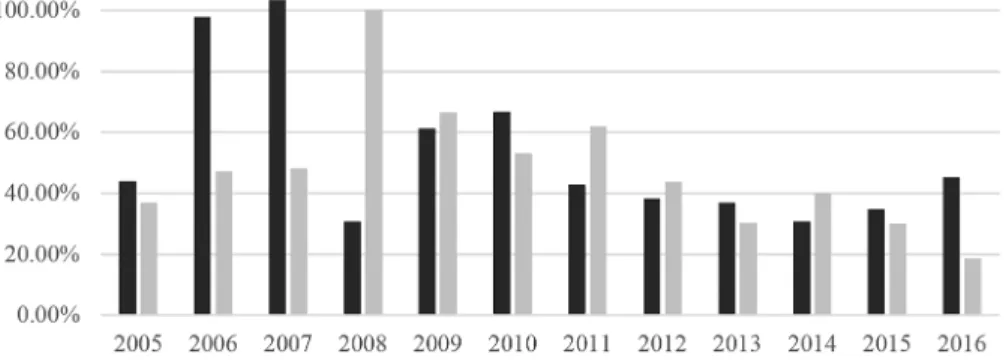
2011. In 2015–2016, the capitalization of Russian companies grew; however, the trading volume decreased, which proves that the activity on the Russian stock market declined (Fig. 2). The capitalization-to-GDP ratio reached 100% in 2006–2007 under the conditions of the rapid growth of both the GDP and mar-ket capitalization, which corresponds to the level of developed countries. How-ever, after the financial crisis of 2008, this ratio decreased from 62% (in 2009) to 32% (in 2014), due to both the GDP growth and the absence of capitalization growth. Therefore, in recent years, the national securities market capitalization-to-GDP ratio diminished. This fact indicates the existence of significant gaps between the capitalization of the stock market and GDP, which also reduces the role of the Russian stock market in the world economy, and makes domestic market unattractive for investors. In 2015–2016, the capitalization-to-GDP ratio increased, partly due to the slowdown in the GDP growth rate.
Figure 2. Capitalization-to-GDP ratio and trading volume-to-capitalization ratio, in %1
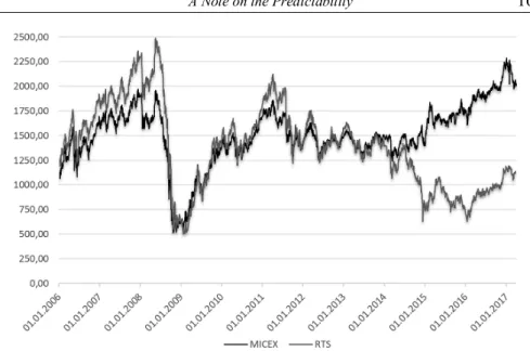
The interest in the Russian securities has gradually recovered since June 2012. At the end of 2016, the main Russian stock market index (MICEX) grew by 3.1%. In January 2013, MICEX grew by 6.18%; however, at the end of the year, it fell by 4.97%. Due to the events in Ukraine and economic sanctions against Russia introduced in 2014, the ruble depreciated considerably and oil prices decreased considerably. These factors contributed to the downfall of the Russian stock market index by 45% at the end of 2014. Figure 3 shows a further decline in MICEX in 2015. Here, it is also important to note that, in 2014–2015, inverse trends of the two main Russian indices MICEX and RTS were observed. This fact was stipulated by the instability and weakness of the Russian currency compared to the U.S. dollar during the period in question and the weakness of the Russian economy in general.
1 Authors’ calculations. Source(s) of data:
Figure 3. Dynamics of RTS and MICEX indices in 2006–20161
National companies’ liquidity (trading volume-to-capitalization ratio) has always been close to its average value of 45% (with the exception of the period of the financial crisis of 2008). However, in 2015–2016, the liquidity of the Rus-sian stock market dropped to 30% and 18.5%, respectively2. This also demon-strates the overall negative trend of the Russian stock market.
Today, about 80% of the trading volume of the Russian stock market is gen-erated by ten largest issuers. The capitalization of the ten largest national com-panies has remained stable over the past five years (around 56% of total market capitalization (Table 1). In 2015, almost half of all transactions in securities was generated by the following three issuers: Sberbank, PJSC; Gazprom, PJSC; and LUKOIL, PJSC.
The number of the listed companies decreased by 7.1% in the period after the sanctions, viz. from 266 companies at the end of 2015 to 247 at the beginning of 2017.
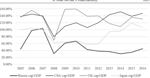
Figures 4 and 5 present the results of a comparative analysis of relative indi-cators of development related to Russia and some developed countries. In devel-oped markets, the turnover-to-capitalization ratio remained on average at 100% or above during the period under study (excluding 2008), whereas, in the Rus-sian market, it fluctuated around 45% (Fig. 4). The capitalization-to-GDP ratio in developed countries was on average 150%; whereas in Russia, the maximum value of 100% was achieved only once in 2008 (Fig. 5).
One of the major disadvantages of the Russian securities market is the com-modity nature of economy. Hence, there is a strong dependence of economic activity on movements of the price of commodities (Fig. 6). The Russian stock
1 Authors’ calculations. Source(s) of data: http://moex.com/en/indices 2 http://moex.com/en/indices
market is also considered to be highly volatile and unstable. With this in mind, we calculated the standard deviation of the monthly returns of MICEX and three foreign indices (viz. FTSE 100, S&P 500 and Nikkei 225) over the period from December 2008 to January 2017. The obtained values of the indicator were 8.39%, 4.3%, 4.71%, and 6.55% respectively.
Table 1. Capitalization of the ten largest Russian public companies in 2015–20161
Company Capitalization, in bln. rub
The share in total capitalization, in % 2015 2016 2015 2016 Gazprom, PJSC 2,957.91 3,589.69 10.2 9.2 NK Rosneft, OJSC 2,489.49 4,187.16 8.6 10.7 Sberbank, PJSC 2,002.96 3,663.19 6.9 9.4 LUKOIL, PJSC 1,835.02 2,879.56 6.3 7.4 NOVATEK, OJSC 1,657.83 2,349.13 5.7 6.0 Norilsk Nickel, PJSC 1,331.16 1,569.34 4.6 4.0 Surgutneftegas, OJSC 1,119.15 1,091.13 3.9 2.8 Magnit, PJSC 964.80 1,018.53 3.3 2.6 VTB Bank, PJSC 941.32 947.98 3.2 2.4 Gazprom Neft, PJSC 668.06 1,011.53 2.3 2.6
The sum total 15,967.70 22,307.22 55.0 57.3
Total capitalization
of MICEX 29,032.88 38 953,42 100.00 100.00
Figure 4. The trading volume-to-capitalization ratio in the Russian stock market compared to the ratio in developed countries’ markets, in %2
1 Authors’ calculations. Source(s) of data:
https://www.investing.com/analysis/stock-markets and http://moex.com/en/indices
2 Authors’ calculations. Source(s) of data: https://data.oecd.org and
Figure 5. Capitalization-to-GDP ratio in the Russian stock market compared to the ratio in developed countries’ markets, in %1
Figure 6. Dynamics of statistical differences for the GDP, the price of Brent, and MICEX in 2008–20162
Given this, during the period under analysis, the volatility of the Russian stock market was almost twice higher compared to the market volatility of the U.K. and the U.S., and 1.3 times higher than the volatility of the Japanese market.
Besides, the Russian stock market is also characterized by low investment activity of companies and private investors. Figure 7 presents data of a compara-tive analysis of the investment-to-GDP ratio in some countries. According to
1 Authors’ calculations. Source(s) of data: http://www.imf.org/en/data and
https://www.world-exchanges.org
2 Authors’ calculations. Source(s) of data: http://www.gks.ru and
this relative indicator, Russia is in a satisfactory situation. On average, in the analyzed period, the share of investment in the GDP in Russia was 20.78%; whereas it was 20.33% in the U.S., 17.29% in the U.K., 21.53% in Japan, 44% in China, 19.09% in Portugal, 20.80% in the European Union. The world’s aver-age was 22.57%. However, given that, in 2016, Russia’s and China’s GDP per capita at current prices had very close values (viz. $ 8,838.2 and $ 8,260.9, re-spectively, according to the OECD data), we can conclude that Russia is charac-terized by low investment activity compared to any other country at a similar stage of development. The remaining countries are characterized by the follow-ing values of GDP per capita: $19,758.7 in Portugal, $ 37,304.1 USD in Japan, $ 40,411.7 in the U.K., and $ 57,293.7 in the U.S.
Figure 7. Share of investments in Russia’s GDP, in %1
Another weak feature of the Russian stock market is the insufficient devel-opment of regional equity markets. Today, there are only 7 operating stock ex-changes officially registered by the Central Bank of the Russian Federation, with MOEX being the largest. The other 5 exchanges are located in Moscow (the capital of the Russian Federation) or Saint Petersburg (the second significant city of the Russian Federation) and specialize predominantly in trading com-modities and raw materials, or currencies. The only regional stock exchange is the Crimean stock exchange, located in Simferopol (the third city of federal sig-nificance). Table 2 presents the share of the capitalization of companies, traded on the central Russian stock exchanges (MICEX or MOEX after reorganiza-tion), in the total market capitalization in the 2011–2016 period. The indicator amounts to 93.3% on average. With this in mind, we shall note that, almost en-tire stock trading in Russia is conducted on the basis of one central exchange platform.
Table 2. The capitalization structure of the Russian stock market, in %1 Year Total market capitaliza-tion, in bln. rub Capitalization of MOEX, in bln. rub Share of MOEX capitali-zation, in %
2011 25,533.9 19,883.9 77.9 2012 25,676.8 24,657.0 96.0 2013 26,247.0 25,255.6 96.2 2014 24,275.6 22,838.2 94.1 2015 29,032.9 28,733.2 99.0 2016 38,953.4 37,748.0 96.9
Many researchers note a сlose correlation and dependence between the Rus-sian stock market and international equity markets. We calculated correlation coefficients between the monthly rates of the returns of MICEX and FTSE 100, S&P 500 and Nikkei 225 over the period from January 2008 to June 2012 and obtained the following values 0.72, 0.72, and 0.69, respectively. In the period from October 2011 to April 2017, the correlation coefficients decreased to 0.41, 0.34, and 0.29, respectively. Hence, we can conclude that there is a positive cor-relation between MICEX and foreign indices. The higher corcor-relations during the 2008–2012 period can be justified by the 2008 crisis, which strongly affected all economies.
The Russian stock market is very young compared to international stock markets. It is characterized by high volatility, instability, and other features: (1) low investment activity of companies and private investors; (2) insufficient de-velopment of regional equity markets; (3) close positive relationship between the Russian and foreign markets; (4) high dependence on commodity prices.
Furthermore, since 2011, the development of the Russian stock market has almost stopped. The absolute indicators characterizing the market scale have remained at the same level, never reaching the value of 2007. The relative indi-cators characterizing the level of the market development and its role in the economy have demonstrated stagnation or a negative trend since 2011. Devel-oped markets continue their upward movement compared to the Russian stock market, which reached the level of developed countries only once, viz. in 2006– 2007.
Methodology In-sample
The empirical part of our study started with in-sample performance evalua-tion of the entire observed sample for the period from January 2008 to January 2017. We used the traditional predictive regression approach, which enabled us to check if there is a linear relationship between the equity premium and the predictors (1), as described by Hong et al. [10].
1 Calculations based on data sources http://moex.com/en/indices and
= + , Predi,t-1+ , + ,, (1)
where is market excess returns over the risk-free rate in month t; Predi,t-1 stands for predictor i with a one-month lag; represents a variable that controls the existence of autocorrelation in the equity premium; and , is the
error term. We are interested in the coefficient , , which indicates the ability of
each predictor to facilitate prediction of the stock market profitability.
The analysis of the predictability of the stock market was performed with the traditional linear predictive regression (ordinary least squared estimation). In the framework of this approach, we used robust standard errors, i.e., corrected for heteroskedasticity and autocorrelation. As software support, Microsoft Excel and Gretl were employed.
In the beginning, the capability of industry returns to predict the movement of the Russian stock market was analyzed. In order to estimate the predictive ability of industries to lead the future stock price of companies, we analyzed 9 portfolios using (1). Eq. 1 was calculated separately for each of the 9 industries, viz. oil and gas, electric utilities, telecoms, metals and mining, manufacturing, finance, consumer goods and services, chemicals, and transport.
Then, we expanded our approach, over other variables and estimated the pre-dictive ability of the following macroeconomic variables: inflation rate, bond yield spread, excess returns of the MICEX corporate bond index, oil price, USD/RUB exchange rate, market volatility index, and dividend yield.
Finally, after estimating 16 predictive regressions using (1), we identified signifi-cant predictors of the Russian stock market. In order to determine the in-sample sig-nificance of the predictors, the standard t-statistic test was performed (2).
t = ^,
^ , (2)
where ^ is an estimated coefficient and ^ is its standard deviation.
Out-of-sample
For predictors identified as significant in the framework of in-sample analy-sis, out-sample performance evaluation was implemented. The total sample was split into the following two periods: (1) from to t, which comprised the ary 2008–December 2013 period, and (2) from t to , which covered the Janu-ary 2013–JanuJanu-ary 2017 period.
First, Eq. (1) was estimated for each predictor using data from the -to-t pe-riod. Then, we calculated the estimated parameters of the regression for the con-stant, the MICEX index and predictors for the period t (December 2013).
Hence, at moment t+1 (January 2014), applying (3), it was possible to predict the MICEX returns, with estimated coefficients for the previous month.
where ^, ^, , and ^, are estimated coefficients and ^ represents a
prediction of the excess returns of MICEX based on predictor i in January 2014.
At the next stage, the procedure was reiterated for all the industries and indi-cators of economic activities, which had exhibited predictive ability in sample, extending the analysis up to the end of the out-of-sample period. Consequently, 37 regression models were estimated for each significant predictor. Finalizing this stage of analysis, predictions of the MICEX returns for the out-of-sample period were obtained, and forecast errors were computed as the difference be-tween the real MICEX returns in the out-of-sample period and the predicted re-turns. We also calculated the mean-squared forecast error (MSFE) of the derived predictive models and the mean-squared forecast error of the historical mean model (4). For the purpose of determining whether our model was close to the actual excess returns, squared errors were calculated.
= ∑ − ^ , , (4)
where ^ , is a prediction of the excess returns calculated for predictor i
over period s+1. The MSFE computation started at moment t+1 and comprised 37 periods.
Then, , pseudo R-squared, was computed out of sample (5). If is posi-tive, the derived model outperforms the prediction based on the historical mean.
= 1 – , (5)
where represents a measure based on the model, and is
the MSFE from the historical mean (calculated as a sum of squared errors for the out-of-sample period).
The out-of-sample predictive ability of predictors can be tested using the MSFE-adjusted test statistic. This test is used to examine the null hypothesis that the unrestricted model MSFE is equal to the constrained model MSFE, whereas the alternative hypothesis says that the first model’s MSFE is lower than that of the latter (6).
^, = − ^ − − ^ , − ^ −
^ , , (6)
where ^ , is a prediction of the excess returns calculated for predictor i at month t based on the model and ^ stands for a prediction of the excess returns at month t based on the historical mean.
The MSFE-adjusted statistic was obtained by performing ^, regression with a constant and applying the resulting t-statistic to a zero coefficient. The null hypothesis of equal forecast ability is rejected at 5% significance level, if the t-statistic exceeds 1.645 (one-sided test).
It is well known that predictions based on a single predictor tend to be exces-sively volatile. With this in mind, we followed Rapach et al. [4] and examined
whether forecast combinations demonstrate a better predictive ability than fore-cast based on a single variable. In this context, we computed the out-of-sample performance of the prediction algorithm based on the simple average of (i) sig-nificant industry predictors, (ii) sigsig-nificant macroeconomic variables and (iii) all significant predictors. For these three obtained forecasts, we also computed the mean-squared prediction error and examined whether the derived mean models were better predictors than the historical mean model.
Utility gains
At the last stage of our calculations, we estimated the utility gains of the mean-variance investor, who has to choose what fraction of his wealth to invest in risk-free assets and the stock market and whether it is profitable for him to use the derived model for the purpose of making an investment decision. Thus, we computed the utility gains of the risk-averse investor who uses prediction of stock returns based on the derived models against the investor who makes his decision with regard to the historical mean. For this purpose, the difference be-tween the average utility of these two investment strategies was calculated (7). The difference should be positive if implementation of a predictive model gen-erates benefits for the mean-variance investor.
= ^ – ^ , (7)
First, we calculated utility for the investor who makes his decisions based on the historical mean model. Here, we determined the share of the investor’s wealth , which optimal to invest in equity at each month t. We considered the mean-variance investor with acoefficient of relative risk aversion, γ, equal to 5.
= ^^
, , (8)
where ^, is the rolling window (72 months) estimate of the variance of stock
returns.
Applying this strategy for predicting excess returns, a mean-variance investor will achieve the average utility given by (9)
^ = ^ – ^ , (9)
where ^ and ^ are the sample average and variance of mean model over the out-of-sample period for an investor’s portfolio formed using only the historical mean model.
Similarly, we calculated the share of investments in equities , and the average utility ^ for the mean-variance investor who makes his decision on the basis of the predictive models (10) and (11):
, = ^ ,
^, , (10)
^ = ^, – ^, , (11)
where ^, is the rolling window (72 months) estimate of the variance of stock
returns, ^, and ^, represent the sample average and variance over the
out-of-sample period for the investor’s portfolio formed using the predictive model.
At the final stage of the evaluation of the mean-variance investors’ utility, we performed a comparative analysis between the utility of predictive models and the utility that an investor would achieve if he decided to fully invest in the stock market (i.e., an investor who chooses weight equal to 1 for all months).
Database
In this study, we analyzed the ability of several variables to predict the equity premium on the Russian stock market over the period January 31, 2008 to Janu-ary 31, 2017. We collected the following monthly data on the MICEX general index returns and several predictors of its change:
- Data on returns of nine industry indices returns, (including oil and gas, electric utilities, telecoms, metals and mining, manufacturing, finance, consumer goods and services, chemicals, and transport.
- Other indicators of macroeconomic activity, such as inflation rate, bond yield spread, the MICEX corporate bond index, the Brent oil price in USD and RUB, USD/RUB exchange rate, market volatility index, and dividend yield.
We examined 16 variables as predictors. MICEX was taken as an indicator of the dynamics of the Russian equity market. It was calculated as a weighted composite index based on the prices of the 50 most liquid Russian stocks of the largest and most dynamic Russian issuers traded on the Moscow Exchange. The MICEX index is denominated in Russian rubles; in contrast, the RTS index, which has the same base of calculation, is denominated in U.S. dollars. We se-lected MICEX as an analyzed index, because it is ruble-denominated and thus free of currency risks and represents the dynamics of the Russian stock market more adequately from the perspective of a Russian investor.
The database was obtained from Thomson Reuters Datastream, Eikon, and the official websites of the Moscow Exchange, the Central Bank of the Russian Federation, the Federal State Statistics Service, and other supplementary statisti-cal sources, including Cbonds, Stock Markets Analysis & Opinion— Investing.com, and the World Federation of Exchanges.
In order to analyze the predictability of the Russian stock market, we per-formed some transformations in the raw data that we had collected:
- The indicator of the Russian stock market performance was computed as a difference between the MICEX monthly returns and the risk-free rate, i.e., one-month Russian bond yield obtained from the Cbonds website.
- For each industry, excess industry returns were calculated as the difference between monthly industry returns and the risk-free rate.
- Bond yield spread was calculated as the difference between the monthly ten-year government bond yield and the risk-free rate.
- The excess returns of the MICEX corporate bond index were calculated as the difference between the monthly returns of the MICEX corporate bond index and the risk-free rate.
- The dividend yield was approximated by the weighted average of the divi-dend yield of the 30 largest companies included in MICEX according to their weights in the index.
- Regarding oil prices and the USD/RUB exchange rate, we used a normal-ized value of these indicators, which had been obtained by dividing indicators’ values at the end of a month by their moving average values over the previous 12 months1.
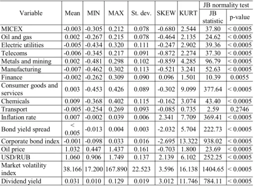
According to Table 3, on average, the mean value of the equity premiums of 9 industry portfolios is 0.003 units, the minimum is -0.332 units, the maximum is 0.289 units. Thus, the mean excess returns of industry indices over the study period is almost equal to zero. The mean value of the MICEX excess returns is -0.003 units, with the minimum of -0.305 units and the maximum of 0.212 units. It proves the overall negative trend of the Russian stock market during the study period. The mean inflation growth over the period under study amounts to 0.007 units per month. The average value of oil price, the USD/RUB exchange rate, the market volatility index, and the dividend yield are equal to 1.032 units, 1.060 units, 38.166 points, 0.031 units per month, respectively, during the study peri-od. In contrast, the dynamics of the excess returns of the corporate bond index is negative (-0.001 units on average per month). The skewness is negative for al-most all the indicators (except the inflation rate, the USD/RUB exchange rate, the market volatility index and the dividend yield), which means that, for most of the indicators, the distributions are left-skewed (right-skewed). All indicators have positive excess kurtosis, which means that the variables have higher proba-bility mass in the tail of their distribution compared to normally distributed vari-ables. In other words, the probability of obtaining extreme values (either very high or very low) is higher. According to the standard deviation value; electric utilities, metals and mining, manufacturing and chemical industries have the highest volatility (0.111 units, 0.102 units, 0.113 units, and 0.116 units, respec-tively). In general, industry indices are more volatile than MICEX (as expected, given that MICEX is more diversified than the industry indices).
The Jarque-Bera normality test demonstrates that the test statistic greatly ex-ceeds the critical value at any reasonable level of significance, i.e., 4.61 at 10% level of significance; 5.99 at 5% level of significance; and 9.21 at 1% level of significance), which makes it possible to conclude that monthly data for almost all the variables do not follow a normal distribution.
1 These variables exhibit a trend. Thus, we have chosen to apply the transformation
Table 3. Descriptive Statistics
Variable Mean MIN MAX St. dev. SKEW KURT
JB normality test JB
statistic p-value
MICEX -0.003 -0.305 0.212 0.078 -0.680 2.544 37.80 < 0.0005 Oil and gas 0.002 -0.267 0.215 0.078 -0.464 2.135 24.62 < 0.0005
Electric utilities -0.005 -0.434 0.320 0.111 -0.247 2.902 39.36 < 0.0005
Telecoms -0.006 -0.345 0.217 0.091 -0.872 2.274 37.30 < 0.0005 Metals and mining 0.002 -0.481 0.298 0.102 -0.859 4.285 96.79 < 0.0005
Manufacturing -0.007 -0.462 0.302 0.113 -0.521 3.241 52.63 < 0.0005 Finance -0.002 -0.262 0.309 0.090 0.096 1.501 10.39 0.0055 Consumer goods and
services 0.003 -0.453 0.426 0.089 -0.302 9.099 377.64 < 0.0005 Chemicals 0.009 -0.368 0.402 0.115 -0.162 3.074 43.40 < 0.0005
Transport -0.005 -0.254 0.269 0.093 -0.085 0.735 2.59 0.2746 Inflation rate 0.007 -0.002 0.039 0.006 2.341 7.709 369.41 < 0.0005
Bond yield spread 0.005 -0.013 0.004 0.003 -2.032 5.704 222.73 < < 0.0005 Corporate bond index -0.001 -0.098 0.033 0.016 -2.695 13.322 938.02 < 0.0005 Oil price 1.032 0.447 1.437 0.161 -0.703 1.800 23.69 < 0.0005
USD/RUB 1.060 0.906 1.749 0.137 2.139 6.102 252.25 < 0.0005 Market volatility
index 38.166 17.200 167.890 22.523 3.596 16.138 1404.65 < 0.0005 Dividend yield 0.031 0.010 0.129 0.019 3.012 11.746 784.11 < 0.0005
The only exception is the transport industry, which has the JB test statistic of 2.59. This value is lower than the critical value with any significance level; therefore, the excess returns of the transport industry can have a normal distri-bution.
Empirical results In-sample results
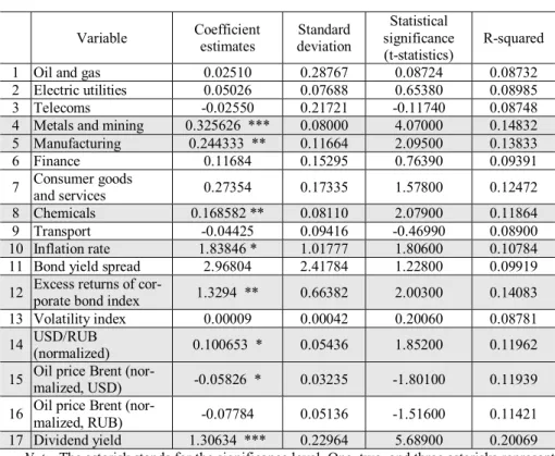
The model presented with (1) was implemented to analyze data on the Rus-sian stock market over the period January 2008 to January 2017. In the frame-work of this model, we employed indicators derived by means of (1), viz. esti-mated coefficients, standard deviations, t-statistics and p-values, and the R-squared for each of the 16 variables. All indicators were analyzed consecutively in order to determine their significance as predictors of the MICEX returns. This procedure was performed using the Gretl software. Table 4 presents regression results obtained by calculating (1) for all the 16 variables. The impact of oil price was estimated twice, denominated in U.S. dollars and Russian rubles. The first 9 variables in the table stand for the indices of industry portfolios; the re-maining variables are macroeconomic indicators.
According to p-value and t-statistics, the most significant variables are the metals and mining industry and the dividend yield (at 1% level of significance).
Table 4. Econometric in-sample results
Variable Coefficient estimates deviation Standard
Statistical significance
(t-statistics) R-squared 1 Oil and gas 0.02510 0.28767 0.08724 0.08732 2 Electric utilities 0.05026 0.07688 0.65380 0.08985
3 Telecoms -0.02550 0.21721 -0.11740 0.08748
4 Metals and mining 0.325626 *** 0.08000 4.07000 0.14832 5 Manufacturing 0.244333 ** 0.11664 2.09500 0.13833
6 Finance 0.11684 0.15295 0.76390 0.09391
7 Consumer goods and services 0.27354 0.17335 1.57800 0.12472 8 Chemicals 0.168582 ** 0.08110 2.07900 0.11864
9 Transport -0.04425 0.09416 -0.46990 0.08900
10 Inflation rate 1.83846 * 1.01777 1.80600 0.10784 11 Bond yield spread 2.96804 2.41784 1.22800 0.09919 12 Excess returns of cor-porate bond index 1.3294 ** 0.66382 2.00300 0.14083 13 Volatility index 0.00009 0.00042 0.20060 0.08781 14 USD/RUB (normalized) 0.100653 * 0.05436 1.85200 0.11962 15 Oil price Brent (nor-malized, USD) -0.05826 * 0.03235 -1.80100 0.11939 16 Oil price Brent (nor-malized, RUB) -0.07784 0.05136 -1.51600 0.11421 17 Dividend yield 1.30634 *** 0.22964 5.68900 0.20069
Note. The asterisk stands for the significance level. One, two, and three asterisks represent significance levels of ten, five, and one percent, respectively.
The manufacturing and chemical industries, the excess returns of the corpo-rate bond index (at 5% level of significance), the inflation corpo-rate, the U.S. dollar-to-Russian ruble exchange rate, and the oil price denominated in U.S. dollars (at 10% level of significance) appear to have predictive power. Consequently, re-garding the metals and mining industry and the dividend yield, we are 99% con-fident that we have obtained regression coefficients that really affect the de-pendent variable. Ultimately, we got three significant industry predictors out of nine and five significant macroeconomic predictors out of eight. Hong et al. [10] revealed that 14 out of 34 industries have an ability to predict one-month ahead market. Hong et al. [10] proved that such indicators as inflation, dividend yield, and market volatility are significant in respect of the U.S. stock market (at 10% level of significance) with the corresponding coefficients -0.578, 1.418, and 0.241, which are close to the values obtained by means of our model (except for the inflation coefficient, which has the opposite sign). Pönkä [6], found that, on the contrary, only a small number of industries are useful in predicting market movements. In the framework of our out-of-sample analysis, three industries proved to have predictive power in relation to excess market returns at 5% level of significance and other three industries at 10% level of significance.
In our study, R-squared values are low for all the predictors (both significant and not significant), which is inherent to this type of studies due to the fact that the equity premium is notoriously difficult to predict. However, significant vari-ables, such as dividend yield, excess returns on corporate bond index, the metals and mining, and manufacturing industries, have the highest R-squared values, viz. 20.1%, 14.1%, 14.8%, and 13.8%. The R-squared values of the remaining variables are, on average, 10.3%. Taking into account that R-squared is a statis-tical measure of how close the fitted data is to the realized equity premium; the higher R-squared value is, the better a model fits data. However, in our example, data inevitably contain a large amount of unexplained variability. Moreover, the study period is characterized by high volatility and variability of the Russian stock market. Even though the R-squared are low, the high t-statistics still indi-cate that there are relevant relationships among the predictors and the dependent variable.
As regards the significant indicators, we suggest that when the metals and mining industry returns increase by 1%, the MICEX returns also increase by 0.326%, ceteris paribus; whereas an increase of 1% in the returns of the manu-facturing industry entails an increase in the MICEX returns by 0.244%, and an increase of 1% inchemicals industry returns leads to an increase in the MICEX returns by 0.169% Thus, metals and mining, manufacturing and chemical indus-tries have a significant positive effect on the MICEX dynamics.
Although the Russian economy and the Russian stock market are strongly dependent on the oil price, it is unexpected that the oil price denominated in Russian rubles and the oil and gas industry are not significant predictors. More-over, due to the fact that Russia is an oil exporter, a rise in oil prices should have a positive impact on MICEX. Significance of the oil price has been confirmed by numerous studies. For instance, Anatolyev [8] found that the oil price had been a significant predictor with a positive effect on the Russian stock market until 2006. Kutan and Hayo [9] revealed that the growth rate of the oil price is a statistically significant predictor with 99% confidence level in in-sample analy-sis (the estimated coefficient is 0.08).
However, it should be noted that the fact that there is a strong contemporane-ous correlation between MICEX and oil prices does not imply that the oil and gas industry or oil prices are a significant predictor. It should be remembered that we use returns of past predictors to forecast the MICEX returns. Therefore, if investors immediately incorporate information from this sector in MICEX, the past industry returns will not be a useful predictor.
The classical theory of economics suggests that in developed countries infla-tion is undesirable but integral to economic growth because it leads to the ex-pansion of production, reduces unemployment, and increases household expens-es. The more profit companies earn, the more the price of stock increases, and the stock market grows in general. Normally, the trends of the stock market and inflation are identical in developed countries. According to the Fisher hypothe-sis, inflation should have a positive effect on the stock price due to the fact that, if the expected real returns are constant, a higher inflation rate implies higher
stock returns. However, there is surprising international evidence that common stock returns and inflation were negatively correlated in the post-war period (Nelson, 1976). The relationship between stock returns and inflation systemati-cally varies in time, depending on the ratio of monetary demand and supply. Applying our model, we have obtained a significant result: an increase of 1% in the inflation rate causes, on average, a 1.84% rise in MICEX per month.
The corporate bond index, as expected, has a positive effect on the MICEX dynamics. Historically bond returns are lower than the returns of stocks; both bonds and stocks compete for the investor’s funds. Thus, if corporate bond re-turns increase, stock rere-turns are to increase, so that stocks remain competitive. In our sample, a 1% growth of returns on corporate bonds causes the MICEX excess returns to increase, on average, by 1.33% per month. A similar effect is expected of the dividend yield: a high dividend yield should predict the high MICEX returns, so this coefficient should be positive. In our model, the rise of the dividend yield by 1% leads, on average, to a 1.31% increase in the MICEX returns per month. Our finding corroborates the study of Fama [2], which sug-gests that stock and corporate bond returns change in the same direction, and the dividend yield move in a similar way under long-term business conditions.
Kinnunen [13] concludes that the predictability of the Russian stock market returns is high. He discovered that the demeaned dividend yield is significant at 10% level of significance (an estimated coefficient of 0.009) and excess oil re-turns is significant at 5% level of significance (an estimated coefficient of -0.257 respectively).
Out-of-sample results and utility gains
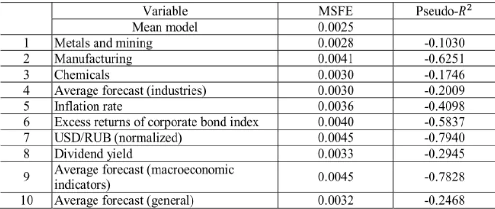
Table 5 shows the MSFE values for the historical mean model and for the significant models (according to (4), (5)). The MSFE values were calculated for the forecast of all eight significant predictors as well as the average forecast of significant industries, the average forecast of significant macroeconomic indica-tors, and all the average forecast of seven significant predictors. The oil price in U.S. dollars was excluded from the calculations due to the fact that the estimated coefficient has an unexpected sign and, therefore, it is economically irrelevant as a predictor. From Table 5, we can see that all forecasts (even the average fore-casts) have a higher MSFE value than the model rested upon the historical mean. Therefore, we have obtained only negative pseudo- for each prediction mod-el, which implies that all the predictions based on the models underperform the predictions based on the historical mean in a mean-squared sense1. Here, it should be noted that the metals and mining as well as chemical industries along-side the average forecast for the industries have the best MSFE value (viz. 0.0028, 0.0030, and 0.0030 against 0.0025 of the historical mean model). The
1 We have not computed the MSFE-adjusted statistic because all the models present a
highest errors are observed in the prediction models based on the USD/RUB exchange rate and the general average forecast (both of 0.0045).
Table 5. Econometric out-sample results
Variable MSFE Pseudo-
Mean model 0.0025
1 Metals and mining 0.0028 -0.1030
2 Manufacturing 0.0041 -0.6251
3 Chemicals 0.0030 -0.1746
4 Average forecast (industries) 0.0030 -0.2009
5 Inflation rate 0.0036 -0.4098
6 Excess returns of corporate bond index 0.0040 -0.5837
7 USD/RUB (normalized) 0.0045 -0.7940
8 Dividend yield 0.0033 -0.2945
9 Average forecast (macroeconomic indicators) 0.0045 -0.7828 10 Average forecast (general) 0.0032 -0.2468
Table 6. Econometric results of utility gains
Variable ^ Variance (^) Utility% Utility differ-ence (mod-mean mod)
Utility differ-ence (mod-full
stock mod) Mean model 0.967% 0.000006 0.966%
Full invested stock m-t model 1.179% 0.002615 0.525% 1 Metals and mining 0.993% 0.000671 0.825% -0.141% 0.300%
2 Manufacturing 0.551% 0.000322 0.470% -0.496% -0.054% 3 Chemicals 1.062% 0.000290 0.990% 0.024% 0.465%
Average forecast
(industries) 0.646% 0.000495 0.523% -0.443% -0.002% 4 Inflation rate 0.615% 0.000621 0.460% -0.506% -0.065% 5 Excess returns of cor-porate bond index 0.646% 0.000357 0.557% -0.409% 0.032% 6 USD/RUB (normalized) 1.083% 0.001676 0.664% -0.302% 0.139% 8 Dividend yield 1.086% 0.000116 1.056% 0.091% 0.532% 9 Average forecast (macroeconomic indicators) 0.098% 0.000761 -0.092% -1.058% -0.617% 10 Average forecast (general) 0.568% 0.000500 0.443% -0.523% -0.082%
Table 6 presents the difference of utility as an economic measure for predict-ing performance (calculated with (7), (9), and (11)) for the mean-variance inves-tor with the risk aversion coefficient equal to five. We are interested in the last
two columns of the table. These columns display the average net benefit per month for an investor who uses the predictive model. The first difference of util-ity was calculated as difference between the average utilutil-ity of the derived model and the average utility of the historical mean model. The fraction of the invest-ment in the stock market in this case was calculated with (10). The data in the last column was calculated as the difference between the average utility of the derived model and the average utility generated for the investor who invests all his funds in the stock market. The last measure is positive for the metals and mining industry, the excess returns of corporate bond index and the USD/RUB exchange rate. The chemical industry and the dividend yield were found the most economically attractive predictors given that they have a positive utility difference in both columns. This indicator can be interpreted as a percentage of the investor’s wealth, which he is willing to pay per month to have access to predictions, generated with the model. For instance, a mean-variance investor with the risk aversion coefficient of five is willing to pay 0.091% of his wealth per month in order to exploit the predictive model based on dividend yield.
Similarly to our study, in Pettenuzzo et al. [5] the economic performance of portfolios was presented based on predictions of out-of-sample returns using a coefficient of risk aversion equal to five. They found a negative utility differ-ence both in the model based on log dividend yield (-0.26%) and in the model based on inflation (-0.09%).
Therefore, evaluating the difference of utility which represents economic gains that can be obtained by an investor who uses the model for the purpose of deter-mining a percentage of wealth to invest in the stock market, we derived 5 models outperforming the strategy that requires all assets to be invested in the stock mar-ket. However, the out-of-sample pseudo R-squared value out-of-sample, as a sta-tistical measure of performance, presents negative results in all the estimated models. Taking the above into consideration, we can conclude that the models underperform predictions based on the historical mean at the statistical level.
Results and Conclusion
Thus, in the course of our study, we have arrived at the following results: 1. The Russian stock market has undergone two major economic crises over the past 17 years. Obviously, it is still characterized by such problems as high volatility, the low level of investment attractiveness and activity, a high degree of dependence on commodity. In general, the Russian stock market is still con-sidered emerging, and the latest trend of the market movement has been nega-tive.
2. Reviewing the economic literature related to the stock market forecasting, we have arrived at the conclusion that the numerous approaches and studies can be grouped under the two main opposing viewpoints: (1) there are certain indi-cators that predict the future returns of the stock market under particular condi-tions; (2) the stock market prices are already adjusted to all the currently availa-ble information; therefore, the future stock price is unpredictaavaila-ble.
3. As regards the Russian stock market, it has been found that the impact of oil prices on the Russian stock market performance is weak and not regular, as confirmed by numerous authors. In fact, the oil price is not a significant predic-tor from 2006 onwards. However, dependence of the Russian stock market on foreign exchanges, such as the U.S. or German exchanges, was proved.
4. Testing the predictability of stock returns with the linear regression esti-mated by OLS, we have identified three out of nine industries and five out of eight macroeconomic indicators as significant predictors. The significant predic-tors (except for oil prices in U.S. dollars) have a positive impact on MICEX.
5. Through the out-of-sample analysis (of the last three observed years), it was found that all models based on significant predictors have higher MSFE than the model rested upon the historical mean (i.e., a negative pseudo- ). This implies that prediction based on models underperforms prediction based on the historical mean.
6. Estimating the mean-variance investor’s utility gains of using predictive models, we have revealed positive utility gains in two out of nine models based on the chemical industry and the dividend yield.
In our research, we have applied an industry-specific and macroeconomic approach to forecasting the Russian stock market for the first time. The results of our study are partly stipulated by the complicatedness of predicting stock market, in general, and by the problems inherent to the Russian stock market. Due to the lack of available data, the time period under study was constrained to a 7-year period for in-sample and a 3-year period for out-of-sample analysis, which is shorter compared to the 20-year period of the full sample. Consequent-ly, the lack of data as well as the high market volatility and uncertainty associat-ed with political and economic shocks (crises) may be partly responsible for the reduced predictive ability of models that we registered in the out-of-sample pe-riod.
Apparently, it is really difficult to predict the stock market movement. Em-ploying only a separate conventional macroeconomic indicator or industry port-folio as a predictor, an analyst encounters the fact that not many of these predic-tors have predictive power. As a rule, implementation of predictive models based on traditional methods (e.g., predictive linear regression) without addi-tional constraints or conditions and techniques fails to outperform the historical mean out of sample.
The open data accessibility for the forecasting model applied in our research weakens by the complexity and longtime calculations for the private investor, as well as by the large deviation of the model’s forecast values from real economic values. Given that, we suppose that, for a private investor, it is easier and more proper to use the moving average method for forecasting and making an invest-ment decision.
As for our model, taking the stated complications into account, we intend to continue our research. The following tasks are to be performed:
- Testing various constraints applicable to the existing OLS models (e.g., positive returns restrictions).
- Calculating the index of the Russian stock market performance (in lieu of MICEX) because it comprises a greater number of Russian shares; thus, it is a more relevant base indicator of a new prediction model.
- Extending the range of predictor indicators that have a significant impact on the Russian stock market.
- Adopting other approaches to predicting the stock market (e.g., the GARCH (generalized autoregressive conditional heteroscedasticity model) model, which is superior to OLS in terms of the quality of prediction).
References
1. Danilova, T. & Danilova, M. (2010) Comparative analysis of household savings and investment decisions in the country context. Economic Analysis: Theory and Practice. 36(210). pp. 6–11. (In Russian).
2. Fama, F. (1989) Business conditions and expected returns on stocks and bonds. Journal of Financial Economics. 25(1). pp. 23–49.
3. Campbell, J. & Thompson, S. (2008) Predicting excess stock returns out of sample: Can anything beat the historical average? Review of Financial Studies. 21(4). pp. 1509–1531.
4. Rapach, D., Strauss, J. & Zhou, G. (2010) Out-of-sample equity premium prediction: Combination forecasts and links to the real economy. Review of Financial Stud-ies. 23(2). pp. 821–862.
5. Pettenuzzo, D., Timmermann, A. & Valkanov, R. (2014) Forecasting stock returns un-der economic constraints. Journal of Financial Economics. 114(3). pp. 517–553.
6. Pönkä, H. (2014) Predicting the direction of US stock markets using industry returns. HECER Discussion Paper. 385. pp. 1–16.
7. Govorkov, B. (2016) Forecasting stock market returns over multiple time horizons. Quantitative Finance. 16(11). pp. 1695–1712.
8. Anatolyev, S. (2008) A 10-year retrospective on the determinants of Russian stock re-turns. Research in International Business and Finance. 22(1). pp. 56–67.
9. Kutan, A. & Hayo, B. (2005) The impact of news, oil prices, and global market devel-opments on Russian financial markets. Economics of Transition. 13(2). pp. 373–393.
10. Hong, H., Torous, W. & Valkanov, R. (2007) Do industries lead the stock market? Journal of Financial Economics. 83. pp. 367–396.
11. Ferreira, M. & Santa-Clara, P. (2011) Forecasting stock market returns: The sum of the parts is more than the whole. Journal of Financial Economics. 100(3). pp. 514-537.
12. Neely, C. (2014) Forecasting the Equity Risk Premium: The Role of Technical Indica-tors. Management Science. 60(7). pp. 1772–1791.
13. Kinnunen, J. (2013) Dynamic return predictability in the Russian stock market. Emerging Markets Review. 15. pp. 107–121.
14. OECD. (2017) Data of the OECD. [Online] Available from: https://data.oecd.org. (Accessed: 12.03.2017).
14. Cbonds. (2019) Indices of bond market. [Online] Available from: http://cbonds.ru/indexes. (Accessed: 15.03.2019).
15. Moscow Exchange. (2019) Moscow Exchange indices. [Online] Available from: http://moex.com/en/indices. (Accessed: 17.03.2019).
16. Central Bank of the Russian Federation. (2019) Statistics of the Central Bank of the Russian Federation. [Online] Available from: http://cbr.ru/Eng/statistics. (Accessed: 16.03.2019).
17. Investing.com. (2019) Stock Markets Analysis. [Online] Available from: https://www.investing.com/analysis/stock-markets. (Accessed: 18.03.2019).
18. World Federation of Exchanges. [Online] Available from: https://www.world-exchanges.org. (Accessed: 15.03.2019).