A Robust Forecasting Framework based on The Kalman Filtering
Approach with a Twofold Parameter Tuning Procedure: Application
to Solar and Photovoltaic Prediction
Ted Soubdhan
a, Joseph Ndong
b, Hanany Ould-Baba
a, Minh-Thang Do
aaUniversity of Antilles, Department of Physics, Laboratory LARGE
bUniversity Cheikh Anta Diop of Dakar, Department of Mathematics and Computer Science, Laboratory LID
Abstract
This paper presents a framework which relies on the linear dynamical Kalman filter to perform a reliable prediction for solar and photovoltaic production. The method is convenient for real-time forecasting and we describe its use to perform these predictions for different time horizons, between one minute and one hour ahead. The dataset used is a set of measurements of solar irradiance and PV power production measured in a sub-tropical zone: Guadeloupe. In this zone, fluctuating meteorological conditions can occur, with highly variable atmospheric events having severe impact in the solar irradiance and the PV power. In such conditions, heterogeneous ramp events are observed making difficult to control and manage these sources of energy. The present work hopes to build a suitable statistical method, based on bayesian inference and state-space modeling, able to predict the evolution of solar radiation and PV production. We develop a forecast method based on the Kalman filter combined with a robust parameter estimation procedure built with an Auto Regressive model or with an Expectation-Maximisation algorithm. The model is built to run with univariate or multivariate data according to their availability. The model is used here to forecast the univariate solar and PV data and also PV with exogenous data such as cloud cover and air temperature. The accuracy of this technique is studied with a set of performance criterion including the root mean square error and the mean bias error. We compare the results for the different tests performed, from one minute to one hour ahead, to the simple persistence model. The performance of our technique exceeds by far the traditional persistence model with a skill score improvement around 39% and 31%, respectively for PV production and GHI, for one hour ahead forecast.
Keywords: Kalman filter, EM algorithm, AR model, Solar Energy, PV forecast.
1. Introduction 1
In sub-tropical zone, such as Guadeloupe, a great challenge related to energy production is to perform accurate
2
solar and photovoltaic (PV) forecast for the purpose to control and manage renewable energy production. This
im-3
portant problem is mostly due to the high variability observed in the solar radiation, since the daily atmospheric
4
conditions (weather, temperature, cloud, etc) encounter many changes for very short time scales. The PV production
5
is thus highly dependent on the meteorological conditions which encounter severe variability in various timescales,
6
from seconds to years. In order to have a good estimation of the PV production, the first problem to solve is to build
7
a suitable solar/PV prevision model able to produce reliable forecasts in order to help energy provider to take control
8
and manage carefully their energy production. One of the great challenge is to provide PV production or global
so-9
lar radiation forecast at a very short timescale under tropical climate. Indeed, large and frequent variations of solar
10
radiation can be observed in tropical climates with amplitudes reaching 800W/m2and occurring within a short time
11
interval, from a few seconds to a few minutes, depending to the geographical location. Such fluctuations can be due,
12
for example, to the dynamic of clouds which can be very complex and depend on cloud type, size, speed and spatial
13
distribution and, more generally, due to some specific local meteorological conditions [26].
14
It is then an important matter to have a good knowledge of these rapid fluctuations occurring on very short time
15
scales and to properly predict the evolution of the solar radiation and the PV production. In addition, the Solar/PV
16
forecasts could be performed with the insertion in the model of the exogenous inputs, i.e. the cloud cover and the
17
ambient temperature to render the whole prediction more robust. Furthermore these predictions can be used as inputs
18
for an infrastructure dedicated to control the PV system. So, in this paper, we implement a robust framework to both
19
predict the solar irradiance and the PV production and try to see the impact of the influential features namely the
20
cloud cover and the temperature. For this scope, we build a methodology based on statistical inference techniques,
21
specifically, the Kalman filtering algorithm. We begin by a learning phase which boils down to defining a convenient
22
state-space model which takes into account the main physical properties of the system of solar and PV power. This
23
state-space model is dedicated to describe the system with all the parameters needed to capture the statistical properties
24
and dynamics of the system. Thereafter, as a second phase, we talk about the methodology to estimate the needed
25
parameters which quantify the dynamics of the system. Finally, we apply the Kalman filter and derive some statistics
26
to analyze the performance of the technique.
27
2. Related works 28
The literature is full of methodologies dedicated to solar and PV forecasting. However, a few of them are based on
29
the robust statistical Kalman filtering technique, which have been extensively used in various scientific areas including
30
signal processing, financial modeling, biology, medicine, aerospace, etc. We have already developed various models
31
with this technique for the scope of anomaly detection in communication networks [15],[16],[17],[18].
32
In the domain of solar/PV forecasting, in [2], a method based on a combination of an ARMA model and a Kalman
33
filter is presented for the scope of solar irradiance and temperature forecasting. The ARMA model is built with
34
a high order parameters (p,q) in order to retrieve the state-space parameters needed to run the Kalman filter. The
35
whole methodology is used to do prediction only for a time horizon of 5 minutes. Another similar technique based
36
on Kalman filtering and ARMA model of high order is presented in [7]. Another study, [4] have presented a work
37
which extends previous studies [5],[20], to solve the problem of bias removal from the Kalman forecasts. However
38
the technique was applied only on ”persistence” model for a time horizon of 1 hour. Generally, ”persistence” forecasts
39
accuracy decrease rapidly with forecast horizon as cloudiness changes severely from one state to another. The works
40
in [5],[13] have developed a linear Kalman filtering model to solve a non-linear forecasting problem. They do so to
41
avoid the parameter tuning operation (estimation of the state system matrix, the observation matrix, and the two
co-42
variance matrices for the state and the measurements) which is a crucial need when using this optimization technique.
43
They should use the extended or unscented Kalman filter to solve the problem, but instead they build a high order
44
polynomial model for the state and set the identity matrix to simplify the state equation. We found that the complexity
45
of this model is high enough and it is not necessary to build at least a 3-rd order polynomial for only the scope of
46
bias removal. In the best of our knowledge, we have found any study referred to the linear Kalman filter which gave
47
a robust parameter tuning procedure before running the technique for the purpose of solar/PV forecasting.
48
In this present work, we build an elaborated method to perform real-time prediction of solar and PV power,
49
based on the knowledge we have on the cloud cover and temperature. The method needs few data for initial parameter
50
estimation. So, all the quantities necessary to run the filter will be identified properly with robust statistical techniques.
51
So an autoregressive (AR) model and a method based on the expectation-maximization algorithm can be suitably used
52
to achieve the parameter settings. On the other hand, our methodology can be applied, with the assumption of the
53
stationarity of the studied process, to do prediction for a various set of time horizons (from 1 minute to 1 hour ahead).
54
The performance level of our methodology is studied with some standard accuracy measures including the root mean
55
square error (RMSE), the mean bias error (MBE) and the mean absolute error (MAE) in their normalized forms.
56
3. Methodology 57
In this work, we aim to build a framework to predict solar radiation and PV power production in real-time
condi-58
tions. The high variability observed in the meteorological conditions (clear sky, cloudy sky, wind speed, temperature,
59
etc) is the principal source of the different levels of variability inside the measured radiance and the PV power. So,
60
it is necessary to have a model able to take the actual data in timetand predict instantaneously the next data at time
61
t+1. One solution to perform this prediction is to consider all the past data up to time timetand perform a prediction
62
for the next timet+1. Techniques as vector autoregressive model (VAR), Wiener filter, etc acts in this way, but the
63
complexity is very high since they use all the past information. These techniques, generally, use much memory to save
64
the history of the data to perform the predictions. Other methods, like first-order Markov model use only the recent
65
arrived data at timetto do the prediction at the next time-step. The Kalman filtering technique performs in this second
66
way. The advantage of using linear discrete-time Kalman filter is mainly related to its ability to do future prediction in
67
real-time conditions for on-line systems in a memory-less way. With this approach, we can build a model from which
68
we derive (estimate) an a priori unknown hidden signal (the underlying real-time hidden system state) and re-utilize
69
it to have our predictions w.r.t. the measured data.
70
We build our forecasting model by assuming that the measured solar/PV power is governed by a hidden signal as
71
in the following linear dynamical system:
72
Yt=AtXt+Vt (1)
whereYt ∈Rmdenotes a stochastic process containing the real measurement (observation) at timet. The stochastic
73
processXt∈Rnis the hidden state of the system which is transformed to the output by the matrixAt ∈Rm×nwhich
74
controls the sources of the measurements. For example, the outputYtcan be composed of the variables: solar
radi-75
ation, ambient temperature, cloud cover, ...;Ytcan also be composed ofmvariables corresponding to the measured
76
solar irradiance or PV power at different points. Generally, due to the intrinsic imperfection of measurement devices,
77
errors more often occur during data collection, thenVtdenotes a stochastic process representing the measurement
78
error.
79
Now we aim to find a convenient model for the stochastic process Xt which is able to track the system traffic
80
features we want to monitor, ie. the estimated solar irradiance and PV production. We propose a simple stochastic
81
model whereXtat discrete timetis represented by the linear combination of two components:
82
Xt=CtXˆt+ξt (2)
where ˆXtis a predictable component,ξtis a random noise component andCt∈Rn×nis a parameter matrix describing
83
the underlying state dynamics.
84
Generally the prediction model can have any structure and the noise process can yield from any distribution.
How-85
ever linear stochastic predictive models combined with gaussian noise have a long record of successful applications in
86
a very large spectrum of engineering techniques. Our idea is to relate the predictable components as networkstates.
87
These variables are not directly observable from the measurement devices, so we refer to them ashidden system states.
88
Since we want to estimate the variablesXtas a state, we can use linear stochastic dynamic system based on state-space
89
models. Now we build a temporal model that relatesXt+1toXtwith the following difference equation:
90
Xt+1=CtXt+BtUt+Wt (3)
where then×nmatrixCtrelates the state at the previous time steptto the state at the current stept+1 andWtis
91
the intrinsic noise process. Here,Ctdescribes the atmospheric conditions since the value of the solar irradiance, or
92
equivalently the PV power, at timetdepend on ambient temperature, cloud cover and wind speed. The value of the
93
solar irradiance betweentandt+1 might change according to that conditions. So we can estimateCtgiven a set of
94
measured data that contains all types of meteorological conditions to train our forecasting model. If one desires to
95
have forecast of the PV power by incorporating in the model other metrics as the temperature, the cloud cover, the
96
wind, etc in order to learn more about their influence for the measures, he/she may take into account the termBtUt,
97
(Bt∈Rn×pandUt ∈Rpwithpexogenous variables). The equations Eq. 1and Eq.3are now combined to form the
98
complete state-space model for the specification of our forecasting framework:
99
(
Xt+1=CtXt+BtUt+Wt
Yt = AtXt+Vt (4)
This block of equations is the classic form for a linear dynamical system with inputs. In this model we assume that
100
the state-noiseWt and the measurement-noiseVt are uncorrelated zero-mean gaussian white-noise processes with
101
covariance matricesQt∈Rn×nandRt∈Rm×m, respectively.
102
4. System parameter tuning 103
Building a framework for multi purpose forecasting might rely on the identification of the needed parameters
104
θ= nCt,At,Qt,Rt
o
for calibrating the evolving system. To achieve this aim, we use two well-known techniques to
105
perform the identification of these parameters before running the filter for forecasting. The first method is based on
106
an autoregressive (AR) model which uses a step-wise least square algorithm performing a QR factorization
(decom-107
position of a matrixTinto a productT=QRof an orthogonal matrixQand an upper triangular matrixR) of a data
108
matrix to evaluate, for a sequence of successive orders, some criterion such as Bayesian Information Criterion (BIC)
109
and Akaike Information Criterion (AIC) for the selection of the model orderp. Thereafter we compute the parameters
110
of the AR model of the optimum order and then retrieve the needed parameterθ. So the matrixCtcan be formed with
111
thepparameters of the AR model. The noise variance of the model is used to fix our system covariance matrixQt.
112
This first model does not give us the matrixRt, so we form it as dependent on the matrixQtsince we know that the
113
intrinsic system noise have an influence to the measurement noise. In practice,Rtis heuristically obtained by dividing
114
the system noise by some constant. To overcome this problem of settingRt manually, we use a second parameter
115
identification algorithm based on the expectation-maximization (EM) algorithm, as we describe in the following.
116
It is important to see that the above parametersθare time-dependent, so they might be calibrated every time data
117
are collected at timet. In this work, we have assumed a stationary case where the parameters are independent of
118
time, and then we perform the calibration only once, with a small part of the training dataset. A procedure of data
119
normalization is presented to accept this assumption.
120
Since we have found a model and system equations for our system, next we need to deal properly with the different
121
steps of our optimization algorithm for solar radiance and PV prediction.
122
5. Prediction equations of the discrete-time Kalman filter 123
The first problem to solve after establishing a real-time state-space model to do our future predictions, is to find an
124
optimal estimate ˆXtof our unobservable statesXt, given a set of measurements{Y1, . . . ,Yt}. In our dynamical linear
125
system, we refer toYtas the observation at timet. And the state of the system at timetis given byXt, let also ˆXt|t
126
denotes the estimate ofXtusing all the information available up to timet. ˆXt+1|tdenotes the prediction ofXt+1using 127
all the information up to timet, (this constitutes thephase predictor). The quantity ˆXt+1|t+1denotes the estimate of 128
Xt+1using all past information and the recently arrived data point at timet+1. On the other hand,Pt|t denotes the
129
error covariance of thestate estimateat timetandPt+1|tindicates the covariance ofthe state predictionat timet+1.
130
If we have the prediction ˆXt+1|t, we plug it into Eq.1to derive a prediction ˆYt+1|tat timet+1.
131
In the above formulation and in the rest of the paper, one should always follow the nuance betweenestimate
132
andprediction. So, at timet, we refer to the quantity ˆXt|t as an estimate and ˆXt+1|t as a prediction. Estimation is
133
instantaneous while prediction is done for the future, given the present.
134
As it is shown in its earlier elaboration, the linear Kalman filter addresses the problem of estimating a discrete
135
state vector when the observations are only a linear combination of the underlying state vector. The filter runs as
136
apredictor-correctoralgorithm. As an iterative algorithm, it estimates the system state using two steps: prediction
137
comes in thetime updatephase, andcorrectionin themeasurement updatephase.
138
• Prediction step(time update equations):
139
In this step, the estimated state of the system at timet, ˆXt|t, is used to predict the state at next timet+1, ˆXt+1|t.
140
And, as we know that the noiseWtinfluences the evolution of the system at each timet, we compute only the
141
covariance of the prediction,Pt+1|tbased on the updated covariance at the previous timet,Pt|t, and the noise
142
covariance at the same time,Qt. The error covariancePt+1|tprovides an indication of the uncertainty associated
143
with the state estimate.
144
( ˆ
Xt+1|t=CtXˆt|t+BtUt|t
Pt+1|t=CtPt|tCTt +Qt
(5)
• Correction step(measurement update equations):
145
This step updates (corrects) the state and the variance of the estimate in the previous step, using a combination
146
of their predicted values and the new observationsYt+1. The correctness of this update depends on the Kalman 147 innovationYt+1−At+1Xˆt+1|t. 148 ˆ Xt+1|t+1=Xˆt+1|t+Kt+1 Yt+1−At+1Xˆt+1|t Pt+1= I−Kt+1At+1 Pt+1|t I−Kt+1At+1 T +Kt+1Rt+1KTt+1 (6)
In the measurement equations,Kt+1 denotes the Kalman gain andIthe identity matrix. For more details in linear
149
dynamical system, estimation and Kalman filter techniques, we refer the reader to [9,8,14]. The above equations
150
with initial conditions of the state of the system ˆX0|0 = E[X0] and the associated error covariance matrix P0|0 = 151
Eh( ˆX0− X0)( ˆX0− X0)T
i
define the discrete-time sequential recursive algorithm for calculating the linearminimum
152
varianceestimate known as theKalman filter.
153
6. Calibration of the Kalman filter 154
In Section3, we have assumed two types of model calibration which can be used to achieve a good prediction.
155
The first method considers that the observation matrixAis precisely known and then we are only interested to find the
156
remaining quantitiesC,QandR. To estimate dynamically these parameters, we use an autoregressive (AR) model.
157
A second, more general model can also be developed, where all the needed parameters,C,A,QandR, are assumed
158
unknown. This method is based on the Expectation-Maximization (EM) algorithm, [6]. This algorithm is an extension
159
of a previously proposed technique, [24,25] where the matrixCis assumed precisely fixed. The work in [6] reinforces
160
this technique by assumingCundetermined.
161
6.1. Parameter Estimation via an AR model
162
The idea behind this parameter estimation technique is to cast an AR model into a state-state form to retrieve the
163
parametersθ. The method is based on a stepwise least squares algorithm which uses a QR factorization of a data
164
matrix to evaluate, for a sequence of successive orders, a criterion (here AIC [1] and BIC [23]) for the selection of
165
the model orderp, and to compute the parameters of the AR model of the optimum order. It is sufficient to learn the
166
model’s parameters using a sample of the first 20-30 days of measurements from the measured data studied. We run
167
this method based on the notes described in [19], and developed in [22]. We form the matrixCusing thepparameters
168
of the AR(p). The noise variance of the model is used to fix the system noise matrixQ. The measurement matrixR
169
cannot be estimated by the AR(p), by experience we take it as a function ofQ. In practice,Ris obtained by dividing
170
the measurement noise by some constant. For our dataset, which is highly variable, we set manually this constant
171
in the interval [0.02; 1.2] for our different experiences. To discover carefully this interval in order to fix the value of
172
R, we run different scenarios of the Kalman filter and choose the value ofRwhich minimizes some optimal criteria,
173
namely the root mean-square error (RMSE) prediction and the mean bias error (MBE) defined respectively as:
174 RMSE= 1 N N X k=1 ( ˆxk−xk)2 1/2 (7) and 175 MBE= 1 N N X k=1 ( ˆxk−xk). (8)
The methodology implemented in [22] is based on the following AR(p) model (which is equivalent to the state
176
equation in Eq.3with the interceptWset to zero):
177
Vr=W+
p
X
l=1
AlVr−l+ǫr, ǫr: is white noise with covariance matrixC (9)
which can be expressed in the form of a regression model of the form:
178
Vr=BUr+ǫr (10)
where the matrixBcontains the parameters to be estimated:
179
B=W,A1, . . . ,Ap
, (11)
and the vectorsUr, of dimensionnp=mp+1 (mis the dimension ofVr), are found as follow:
180 Ur= 1,Vr−1, . . . ,Vr−p (12) Transforming an AR model into a regression model is, in fact, a simple approximation. Indeed, for a regression model,
181
the predicatorsUrare supposed to be constant, while in an AR model, these vectors are the realization of a stochastic
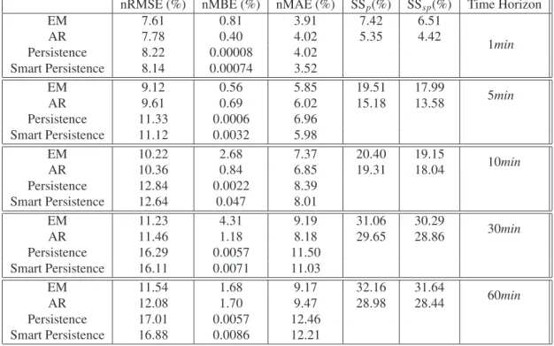
182
process. Then, the approximation needs to have an initial predicatorU1in order to initialize the AR model:
183 U1 = 1,V0, . . . ,V1−p (13)
So, the final step of the QR factorization gives us the matrixCas:
184 C= A1 A2 A3 . . . Ap Id 0 0 . . . 0 0 Id 0 . . . 0 .. . . .. . .. . .. ... 0 . . . 0 Id 0 , (14)
whereId is the identity matrix and theAi are the coefficients of the AR(p). By retrieving a set of quantities, our
185
co-variance matrixQcan be obtained by the formula:
186
ˆ
Q= 1
N−np
(−WU−1W′) (15)
with the following matrices of moments:
187 U= N X r=1 uru′r, V= N X r=1 vrv′r, W= N X r=1 vru′r. (16)
This AR transformation does not give us directly the observation matrix A needed in equation Eq. 4. After
188
retrieving the states matrices with the AR(p), it is obvious to re-transform this AR model in the form of a state-state
189
model. And then the state equation can be plug into the observation equation in order to retrieve the observation
190
matrix.
191
6.2. Parameter Estimation via the EM algorithm
192
Parameter estimation via the EM algorithm boils down, first to combining the state variable Xt and the state
193
noiseWtas a single random gaussian process, and doing the same transformation for the output variableYtand the
194
measurement noiseVt. So with equation Eq. (4), we can form the conditional probability densities for the state and
195
the output of the system as follow (in the following we use respectivelyxtandyt for the state and the measurement
196
vectors for notation convenience):
197 P(yt|xt)= √ 1 (2π)p|R|exp ( −1 2 yt −Cxt′R−1yt −Cxt ) (17) 198 P(xt|xt−1)= 1 p (2π)k|Q|exp ( −12[xt−Axt−1] ′ Q−1[xt−Axt−1] ) (18) where the notation|R|and|Q|are respectively the determinants of the matricesRandQ.
199
Suppose the output of the system is of the form of a multidimensional array withT vectors (y1,y2, . . . ,yT). Let’s
200
denote{y}that observation sequence and{y}t1
t0 being the sub-sequence yt0,yt0+1, . . . ,yt1
. The state equation of the
201
model in Eq.4is a first-order Markov process, so:
202 P{x},{y}=P(x1) T Y t=2 Pxt|xt−1 T Y t=1 P(yt|xt). (19)
If we suppose that the initial state is a gaussian random process of expectationπ1and co-variance matrixV1given by:
203 P(x1)= 1 p (2π)k|V1|exp ( −1 2[x1−π1] ′ V−11[x1−π1] ) , (20)
we can write the logarithm of the jointly probability density between{x}and{y}, as a quadratic sum of terms in the
204 form: 205 logP{x},{y}=− T X t=1 1 2[yt−Cxt] ′ R−1[yt−Cxt] ! −T 2 log|R| − T X t=2 1 2[xt−Axt−1] ′ Q−1[xt−Axt−1] ! −T−1 2 log|Q| −12[x1−π1] ′ V−11[x1−π1]− 1 2log|V1| − T(p+k) 2 log 2π (21)
Our linear dynamical system can be seen as a continuous state of a hidden Markov model (HMM) [21]. Then, the
206
”forward” part of the ”forward-backward” algorithm for a HMM can be established by a Kalman filter, whereas the
207
”backward” part is solved by a recursive ”Kalman smoother” [14]. Finally, if we take into account the measurements,
208
we run the forward-backward algorithm and we solve the problem of inferring the above probability densities for the
209
system state; this operation is done via the Kalman smoother and constitutes the ”E” step of the EM algorithm. To
210
derive this step, we need the three following quantities:
211 ˆ xt≡Ext |{y}, (22) 212 Pt≡Extx′t|{y} (23) 213 Pt,t−1≡E h xtx′t−1|{y}i (24)
The term ˆxt gives an estimate of the system state given the past and future observations, then it differ to the state
214
estimate given by a standard Kalman filter, where this estimate is given by (E[xt|{y}t
1). Thereafter, we can calculate
215
the log-likelihood defined by:
216
L(θ)=EhlogP({x},{y})|{y}i. (25) By setting the quantitiesxτt =Ehxt|{y}τ1iandVτt =Varhxt|{y}τ1i, we can establish the Kalman filter equations for the
217
estimation of our parameters, as follow:
218 xτt−1 = Axτt−−11, (26) Vtτ−1 = AVτt−−11A′+Q, (27) Kt = Vτt−1C ′ (CVτt−1C′+R)−1, (28) xτt = xτt−1+Kt(yt−Cxτt−1), (29) Vτt = Vτt−1−KtCVτt−1. (30) 7
To find ˆxt≡xTt andPt≡VTt +xTt(xTt)′, we need the variables: 219 Jt−1 = Vtt−−11A ′ (Vtt−1)−1, (31) xtT−1 = xtt−−11+Jt−1(xTt −Ax t−1 t−1), (32) VTt−1 = Vtt−−11+Jt−1(VTt −Vtt−1)J ′ t−1. (33) (34) The quantityPt,t−1≡VTt,t−1+x T t(xTt−1) ′
is needed and can be obtained by deriving:
220 VTt−1,t−2=Vtt−−11Jt′−2+Jt−1(VTt,t−1−AV t−1 t−1)J ′ t−2. (35)
The ”M” Step maximizes the likelihood of observing the parameterθ= (C,A,R,Q, π1,V1). Each term of this
221
parameter is derived by considering the partial derivative corresponding to the logarithm of the likelihood. It suffice
222
to put this derivative to zero and resolve the resulting equation, and finally, we find the value of the given parameter:
223
- the observation matrix is given by:
224 ∂L(θ) ∂A =− T X t=1 R−1ytxˆ′t+ T X t=1 R−1APt=0 (36) 225 Anew= T X t=1 ytxˆ′t T X t=1 Pt −1 (37) - the co-variance of the observation noise is derived as:
226 ∂L(θ) ∂R−1 = T 2R− T X t=1 1 2yty ′ t−Cxtyˆ ′ t+ 1 2CPtC ′! =0 (38) 227 Rnew= 1 T T X t=1 (yty′t−C new ˆ xty′t) (39)
- the system state matrix is equal to:
228 ∂L(θ) ∂C =− T X t=2 Q−1Pt,t−1+ T X t=2 Q−1CPt−1=0 (40) 229 Cnew= T X t=2 Pt,t−1 T X t=2 Pt−1 −1 (41) - and the state noise co-variance is given by:
230 ∂L(θ) ∂Q−1 = T −1 2 Q− 1 2 T X t=2 Pt−CPt−1,t−Pt,t−1C ′ + CPt−1C ′ = T−1 2 Q− 1 2 T X t=2 Pt−Cnew T X t=2 Pt−1,t =0 (42) 231 Qnew= 1 T−1 T X t=2 Pt−Cnew T X t=2 Pt−1,t (43) 8
- the initial system state can also be estimated by the quantity: 232 ∂L(θ) ∂π1 =( ˆx1−π1)V −1 1 =0 (44) 233 πnew1 =xˆ1. (45)
- and the initial co-variance given by:
234 ∂L(θ) ∂V−1 1 =1 2V1− 1 2 P1−xˆ1π ′ 1−π1xˆ ′ 1+π1π ′ 1 =0 (46) 235 Vnew1 =P1−xˆ1xˆ ′ 1. (47)
7. Forecasting criterion of accuracy 236
To evaluate the performances of our model, we use several accuracy measures defined to evaluate solar and PV
237
forecasts. Benchmarking of solar forecasts has been examined by the International Energy Agency Solar Heating and
238
Cooling Program Task 36 on ”Solar Resource Knowledge Management” and the project ”Management and
Exploita-239
tion of Solar Resource Knowledge,” which have suggested guidelines for performance analysis of the forecasting
240
models [12]. Solar and PV forecast accuracy was assessed in terms of RMSE, mean absolute error (MAE), and mean
241
bias error (bias) MBE. RMSE gives more weight to large errors, whereas MAE, less sensitive to large errors, reveals
242
the average magnitude of the error, and MBE indicates whether there is a significant tendency to systematically
over-243
forecast or under-forecast. When comparing between different models in the training year, RMSE was used as the
244
metric for minimization, that is, forecasts were trained with the goal of reducing the largest errors. These performance
245
criterion are used here in the normalized forms defined as follow:
246 nRMSE= v t 1 N N X i=1 (Pi−Pi)ˆ 2 max(Pi)−min(Pi) (48) 247 nMAE= 1 N N X i=1 |Pi−Piˆ| max(Pi)−min(Pi) (49) 248 nMBE= 1 N N X i=1 (Pi−Pi)ˆ max(Pi)−min(Pi) (50)
We also include a new metric: the forecast skill score (SS) parameter. The latter proposed by Coimbra et al.,[3]:
249
SS=1−RMSEforecast
RMSEsc-pers
(51) The skill score gives the fractional improvement in the mean square error of the proposed forecasting model over
250
the reference model (here the ”persistence” model): a skill score of 1 indicates a perfect forecast, a score of 0 indicates
251
no improvement against the reference, and a negative skill means that the forecast model tested performs worse than
252
the reference.
253
8. Forecast methods 254
8.1. Basic persistence
255
The Kalman filter forecasting technique is compared against the classical scaled persistence model. It is based on
256
the assumption that the current conditions will persist so that,
257
ˆ
Ip(t+T)=Ip(t) (52)
where ˆIp(t+T) represents a GHI prediction from the persistence model,T represents the forecast horizon, andIp(t)
258
is the measured GHI value at timet.
259
8.2. Smart persistence
260
Our forecasting approach is also compared with the smart persistence. The smart persistence model is based on
261
the same assumption as persistence model but it corrects for the deterministic diurnal variation in solar irradiance. It
262
is defined as,
263
ˆ
Isp(t+T)=kc(t)Ics(t+T) (53)
where ˆIsp(t) represents a GHI prediction at timet,Ics(t) represents the estimated clear sky solar irradiance [11].
264
9. Validation of the approach 265
9.1. Experimental data
266
9.1.1. Solar and weather data
267
The solar data was measured at the campus Fouillole of the University of the French West Indies and Guiana with
268
the interval of 1 second from 2010 to 2014. In this paper we show only the results concerning one year (2011) which
269
constitutes a complete record of measurements. Before applying the whole methodology and in order to perform
270
forecasts with many time horizons, we have build a pre-processing normalization technique to organize the data into
271
different time-scales with time horizons including 1, 5 and 10 minutes bin increment. The normalization method is
272
exposed in section9.2. We retrieve then the deterministic component of the signal and obtain consequently a stationary
273
process.
274
9.1.2. PV data
275
The PV system studied in this paper is installed on the roof of a storehouse in Guadeloupe. The system has 238
276
flexible PV modules Unisolar of 136Wp each (total of 32,3 kW installed) . The system consists of two inverters of
277
15 kW and 20 kW. The data logging of PV output power (in W) is integrated in these inverters (collected every 5
278
min). For the objective of forecasting, a weather station has been also installed on the roof of the storehouse in 2014.
279
However the duration of data is not long enough and therefore will not be used in this study. The time series data is
280
collected in 2 years: 2012 and 2013. However, due to some errors in the data acquisition of the PV output power,
281
only a collection of data covering 696 days is available. As during the night, the forecast is not necessary because the
282
output power of PV is zero, the study takes into account only the data between 0700 and 1700 LST every day.
283
The two exogenous variables, cloud cover (in octa) and ambiance temperature (in◦C) are measured on an hourly
284
basis at the Meteo France meteorological station of le Raizet (16◦26N, 61◦24W, 11m asl). The daily average for the
285
solar load on a horizontal surface is around 5 kWh/m2. A constant sunshine combined with the thermal inertia of
286
the ocean makes the air temperature variation quite weak, between 17◦C and 33◦C, with an average of 25◦C to 26◦C.
287
Relative humidity ranges from 70% to 80%, and the trade winds are relatively constant all along the year. Two main
288
regimes of cloudiness are superposed: the clouds driven by the synoptic conditions over the Atlantic Ocean and the
289
orographic cloud layer generated by the local reliefs.
290
9.2. Procedure of the data normalization
291
As the irradiation and the PV production depend on the sun path during the day, a normalization is needed to
292
eliminate this subordination and accept the assumption we have made in the introduction about the stationarity of the
293
signal.
294
In this study, the irradiation will be normalized by the the theoretical clear sky, GHIcskcurve. The Global
Hor-295
izontal Irradiance (GHI) is the total amount of shortwave radiation received by a horizontal surface on the ground,
296
which consists of the direct irradiance and the diffuse irradiance. The GHIcskis the GHI calculated in the condition
297
of clear sky, using the Kasten clear sky model. This model accounts for atmospheric turbidity and solar elevation
298
angle. The inputs to this model are air mass, Linke Turbidity, and elevation [10]. The Linke turbidity factor is a very
299
convenient approximation to model the atmospheric absorption and scattering of the solar radiation under clear skies.
300
It describes the optical thickness of the atmosphere due to water vapor and the aerosol particles relative to a dry and
301
clean atmosphere. With larger Linke turbidity, there is more attenuation of the radiation by the clear sky atmosphere.
302
We obtain then the clear sky index,kc, defined as:
303
kc(t)= GHI(t)
GHIcsk(t) (54)
The input of the PV production at time (t) is then normalized into ¯P(t), the normalized value of the PV production
304
with respect to the maximum value at time (t),Pmax(t).
305
¯
P(t)= P(t) Pmax(t)
(55)
This maximum value can be evaluated from the GHImaxcurve with the following equation:
306
Pmax(t)=
GHIcsk(t)
max(GHIcsk)PVinstalled (56)
9.3. Summary of the results for the different forecast schemes
307
This work aims to show the ability of the Kalman filter to perform reliable predictions of solar irradiance and PV
308
power production. We have proposed two parameter identification techniques, namely the AR model and the EM
309
algorithm, which can be used successfully to calibrate the optimization method for the forecasting.
310
9.3.1. Initialization phase
311
First, in order to run the AR and the EM initialization, we need only a few set of training data. The Kalman filter
312
is an algorithm which performs prediction in the sense of a first-order Markov process. This means that it does not
313
consider all the past information up to timetto give an estimate for timet+1. Instead, we need only the arrived data
314
at timetto have a prediction at the next time step, so we say that the algorithm performs a one-step ahead prediction.
315
Another interesting feature about the Kalman filter is in its feedback nature; it is able to do robust prediction with
316
a strong potential to reducing error estimates by minimizing the variance of this error (with the help of the Kalman
317
gain). So, for our training data, for all variables, we consider a short time-interval formed with the first 20-30 days
318
of year of the data. And the initial parameters are set at the beginning once a time (since we assume stationary of
319
the underlying process) with this part of the dataset. For all our implementations, we have built anAR(1) which is
320
convenient to perform our forecasts, the measurement dataset consisting of a single vector. The rest of the data serves
321
as test data.
322
The obtained initial parameters are then used to perform the calibration of the Kalman filter by running the
323
predictor-corrector phases as described in Section5.
324
We plot, in Figure1, the measured GHI data and the clear sky index, for four days, to give an overview of the
325
fluctuations of the solar irradiance, observed at 1 second time horizon.
326
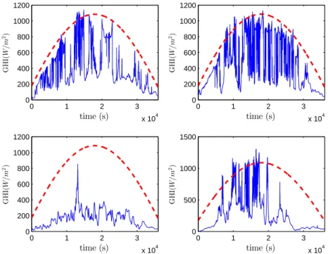
0 1 2 3 x 10⁴ 0 200 400 600 800 1000 1200 time (s) G H I( W /m 2) 0 1 2 3 x 10⁴ 0 200 400 600 800 1000 1200 time (s) G H I( W /m 2) 0 1 2 3 x 10⁴ 0 200 400 600 800 1000 1200 time (s) G H I( W /m 2) 0 1 2 3 x 10⁴ 0 500 1000 1500 time (s) G H I( W /m 2)
Figure 1. Variability of the GHI data, for 4 typical days. The blue line is the measured GHI and the dashed red line is the estimated clear sky with the Kasten model. Time Horizon is 1 second. These figures shows how fluctuating is the solar radiation, with ramps rates of about 800W/m2.
9.3.2. Data preprocessing
327
Before applying the whole procedure, we process the data to ensure it meets all the necessary assumption, i.e. the
328
stationnarity of the underlying process. So, we apply the normalization procedure as described in Section9.2. The
329
PV data set is collected at 1 second timestamp and after we average it at a 1 hour bin increment. For the solar data, we
330
have collected it also at 1 second and then, we make several averages for 1, 5, 10, 30 and 60 min. So, the Kalman filter
331
is applied on the normalized data and thereafter, we reconsider the original signal without normalization, to build the
332
final result and compute the performance measures. The exogenous variables are available only for the PV data.
333
9.3.3. Results obtained for the PV data without the exogenous variables
334
First, we deal with the PV forecast without the knowledge we have on the two exogenous variables, the ambient
335
temperature and the cloud cover. The results are shown in the graphs of Figure. 2(a)and the asbolute error is shown
336
on figure3(a). For the scope of comparison, we plot the forecasts performed with the parameter tuning done by the
337
AR and the EM algorithms. The Kalman filter is, first, applied to the normalized data and we apply the results to the
338
real measurements i.e the not-normalized dataset. We can see that the predicted signal is a good forecast of the real
339
PV at future horizon. The accuracy measures are confined in Table1, with a nRMSE of 8.29% and 8.87% respectively
340
for the EM and the AR calibration models. Globally the table says that the initialization method based on the EM
341
algorithm is a little bit more efficient than the AR model calibration, but the mean absolute error introduced by the
342
EM technique is more important than for the AR case, with the nMAE reaching 4.72% for EM versus 4.61% for
343
AR. Another important issue is related to the performance gained with these technique above the classical persistence
344
model, which gives us a nRMSE of 13.35%. Comparing the method against the basic persistence model, the two
345
initialization methods give a skill score of 33.56%, for the AR and, 37.90% for the EM. Against the smart persistence,
346
our forecasts gives a skill score slightly less, with 32.39% for the AR model and 36.81% for the EM technique. The
347
difference between the two persistence models is not large since, the smart persistence model performs with slightly
348
less error (nRMSE) than the basic persistence. In Figure.2(d), we plot the measured versus predicted PV power and
349
the linear polynomial fitting to show globally the modest performance of the EM initialization above the AR model.
350
Both for all cases, at least 80% of the data are in accordance with the fit, thus we can consider that the two methods
351
are satisfactory.
352
9.3.4. Results obtained for the PV data with the exogenous variables
353
In this study we were also interested in doing forecast for the PV with the knowledge of the exogenous variables,
354
the temperature and the cloud cover which are taken as inputs. So we consider our system of Eq. 4with the input
355
BtUtcontaining the two variables. The matrixBtis obviously set to the identity matrix since each variable is collected
356
in a single point as an unique data vector. If, for example, the temperature were measured at different geographical
357
areas, thus, the matrixBt would be used properly to identify the source of the data each time step. The results are
358
depicted in graphs of Figure. 2(b)and Figure. 2(c). Here, we plot the results to show how each given initialization
359
procedure performs individually with and without the temperature and the cloud cover. The accuracy measures are
360
depicted in Table1. Here we obtain a nRMSE of 8.03% and 8.77% respectively for the EM and the AR initialization
361
techniques. Also we show that each of the techniques performs slightly better with the inputs in terms of root mean
362
square error, than without these exogenous variables. Nevertheless, the results are more sensitive to bias but, the
363
mean absolute error is less than for the case we run the algorithm without the inputs features. For example, for the
364
AR model without inputs, the nMBE and nMAE values reach respectively 0.45% and 4.61% vs 1.81% and 4.18%
365
with the exogenous inputs. The EM algorithm gives, for the model with inputs, a nMBE of 0.42% and a nMAE of
366
4.57% against a nMBE of -0.08% and a nMAE of 4.72% for the model without inputs. Since the PV production
367
depends strongly to the atmospheric conditions, it is very important to be able to do the prediction by incorporating
368
this features in the model. We can accept that the results with inputs are more biased since the temperature and the
369
cloud cover does not evolve in the same fashion and they might influence the production differently making the bias
370
more important. Globally the results found by the two initialization procedures are good with a not negligible benefit
371
for the EM which give less errors than the AR model and than with the same technique used without the exogenous
372
variables. However the EM method is always more sensitive to bias. This model with exogenous inputs is also better
373
than the basic persistence model with an improvement of the skill score which belongs between 34.31% and 39.85%.
374
Also, we obtain better results against the smart persistence with a skill score of 33.16% and 38.80%, respectively for
375
the AR and EM initialization models. The only point where the persistence model outperforms our model is about the
376
bias, which is casually nonexistent.
377
9.3.5. Results obtained for the solar data (GHI) without exogenous variables
378
For the solar data, we have not at hand the exogenous variables. These variables are only available for the PV data.
379
For this data, we have done the calibration for time horizons 1, 5, 10, 30 and 60min but, for the scope of illustration,
380
we plot,in graphs of Figures4(a),4(b), only the results for time horizons 30 and 60 minutes, respectively. On figure
381
3(b)the asbolute error is shown for a time horizon of one hour. As for the previous results about the PV forecasts, the
382
EM and AR techniques give good performance with a nRMSE in the interval [7.61%; 12.58%] against a nRMSE in
383
the interval [7.79%; 16.94%] for the persistence model. We have almost the same results by comparing the obtained
384
results with the smart persistence model. Comparing our two tuning algorithms, as we observe in Table2, the three
385
accuracy measures gives better for the EM than for the AR in terms of nRMSE. In Figure.4(c), we find the trade-off
386
between the measured and the predicted solar irradiance and their polynomial fit of degree 1. More generally, the two
387
different initialization techniques give globally good results and they can be used according to the need and objective
388
of the engineer, to do forecasting with several time scales. The results obtained for very short time scales (1, 5, 10min)
389
has a skill score between 5.35% and 20.40%. These results are interesting since for short time scale we have very
390
strong flcutuating conditions.
391
The performances with the time horizons 30 and 1H are much better than the persistence models; we can achieve
392
an improvement with a skill score of 32.16% and 31.64% respectively for the basic and the smart persistence models.
393
This results are promising since we are in presence of high fluctuating meteorological conditions for which it is not
394
obvious to gather all the knowledge in order to reduce subsequently the error and the bias of the evolving process
395
being modeled.
396
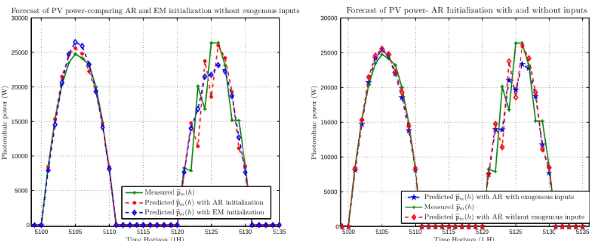
5100 5105 5110 5115 5120 5125 5130 5135 0 5000 10000 15000 20000 25000 30000 Time Horizon (1H) P h ot ov ol tai c p ow er (W )
Forecast of PV power-comparing AR and EM initialization without exogenous inputs
Measuredbpm(h)
Predictedbpm(h) with AR initialization
Predictedbpm(h) with EM initialization
(a) Comparison of the two models AR and EM. The EM initial-ization model gives more reliable results than the AR.
5100 5105 5110 5115 5120 5125 5130 5135 0 5000 10000 15000 20000 25000 30000 Time Horizon (1 H) P h ot ov ol tai c p ow er (W )
Forecast of PV power- AR Initialization with and without inputs
Predictedbpm(h) with AR with exogenous inputs
Measuredbpm(h)
Predictedbpm(h) with AR without exogenous inputs
(b) The AR model performs slightly better with exogenous variables than without these features.
50950 5100 5105 5110 5115 5120 5125 5130 5135 5000 10000 15000 20000 25000 30000 Time Horizon (1H) P h ot ov ol tai c p ow er (W )
Forecast of PV power-EM initialization with and without exogenous inputs
Measuredbpm(h)
Predictedbpm(h) with EM initialization with input
Predictedbpm(h) with EM initialization without inputs
(c) The EM model performs slightly better with exogenous variables than without these features.
0 5000 10000 15000 20000 25000 30000 35000 0 5000 10000 15000 20000 25000 30000 35000 Predictedbpm(h) W P re d ic te d b pm ( h ) W
Measured vs Predicted PV- without inputs
0 5000 10000 15000 20000 25000 30000 35000 0 5000 10000 15000 20000 25000 30000 35000 P re d ic te d b pm ( h ) W Measuredbpm(h) W
Measured vs Predicted PV- with inputs Temperature and Cloud Cover
AR initialization EM initialization linear Fit (EM) linear Fit (AR)
y(x) = a x a = 0.92181 R = 0.86503 (lin) y(x) = a x a = 0.9488 R = 0.85561 (lin) y(x) = a x a = 0.97422 R = 0.84739 (lin) y(x) = a x a = 0.97022 R = 0.84436 (lin)
(d) Plot of the measured vs predicted PV data to show the perfor-mances of the two tuning algorithms, namely, AR and EM.
Figure 2. The graphs show the Kalman filter forecast for the PV data at time horizon 1H. In Figure (2(a)), we compare the AR and EM algorithms to show which one gives better results. In Figure (2(b)) and (2(c)) we plot the results for, respectively, the AR and EM models for parameter initialization, when we take into account the exogenous inputs (cloud cover and ambient temperature). In graph of Figure (2(d)) we measure and compare the performance of each initialization method w.r.t. the fit along with a 1-st order polynomial function.
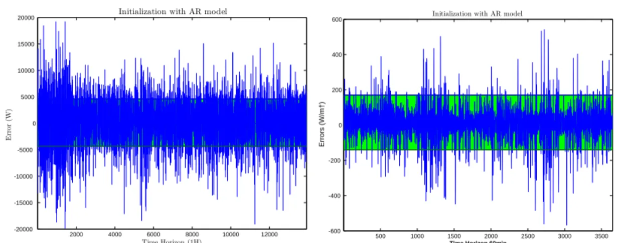
2000 4000 6000 8000 10000 12000 -20000 -15000 -10000 -5000 0 5000 10000 15000
20000 Initialization with AR model
Time Horizon (1H) E rr or (W )
(a) Forecast errors of the PV at Time Horizon 1H for one year of data. AR model. 500 1000 1500 2000 2500 3000 3500 -600 -400 -200 0 200 400
600 Initialization with AR model
Time Horizon 60min
Errors (W/m†)
(b) Forecast errors of the GHIat Time Horizon 1H for one year of data.
Figure 3. Kalman filter prediction absolute errors obtained with AR initialization methods for time horizon 1H, PV and solar. We have calculated and represented (green interval) the 95% confidence interval around the mean.
Table 1. Comparison of the different performance criterion for the different prediction models for the real PV with and without the exogenous inputs Temperature and the cloud cover. SSpis the skill score calculated for the basic persistence model and SSspthe skill score for the smart
persistence. Time Horizon 1H.
Without exogenous inputs
nRMSE (%) nMBE (%) nMAE (%) SSp(%) SSsp(%)
EM 8.29 -0.08 4.72 37.90 36.81
AR 8.87 0.45 4.61 33.56 32.39
Persistence 13.35 0.00024 8.13
Smart Persistence 13.12 0.0084 8.04
With exogenous inputs
EM 8.03 0.42 4.57 39.85 38.80
AR 8.77 1.81 4.18 34.31 33.16
10. Conclusion 397
We have presented in this work a robust forecasting method based on the Kalman filter combined with a
prob-398
abilistic initialization, Expectation Maximisation (EM) or Auto Regressive (AR) based. The model is built to be
399
performed with both univariate or multivariate data. We test here it’s ability to forecast solar radiation from 1 minute
400
to one hour ahead, and photovoltaic power production for one hour ahead. The influence of exogenous inputs on the
401
forecasting error is also evaluated. And finally we compare the forecasting errors to those obtained with the naive
402
persitence model.
403
The proposed technique begins with the establishment of a dynamical state-space model able to capture the
dy-404
namics of the system we want to monitor. Thereafter, we propose different algorithms for the scope of parameter
405
identification, since a great challenge in order to run properly the Kalman filter is the discovery of the initial values
406
of the system quantities. A thorough description is performed about the usage of the defined system in its state-space
407
form formulation which could help for system identification.
408
On the other hand, our state-space model is defined in a more elaborated form, convenient to including all the
409
matrices which govern the whole system and which have a great importance to incorporate the relevant knowledge
410
(features) to perform a suitable forecasting operation. Thereafter, the difficult and challengeable task of parameter
411
tuning is overcome with two robust optimization techniques, namely the EM algorithm and the AR model, based on
412
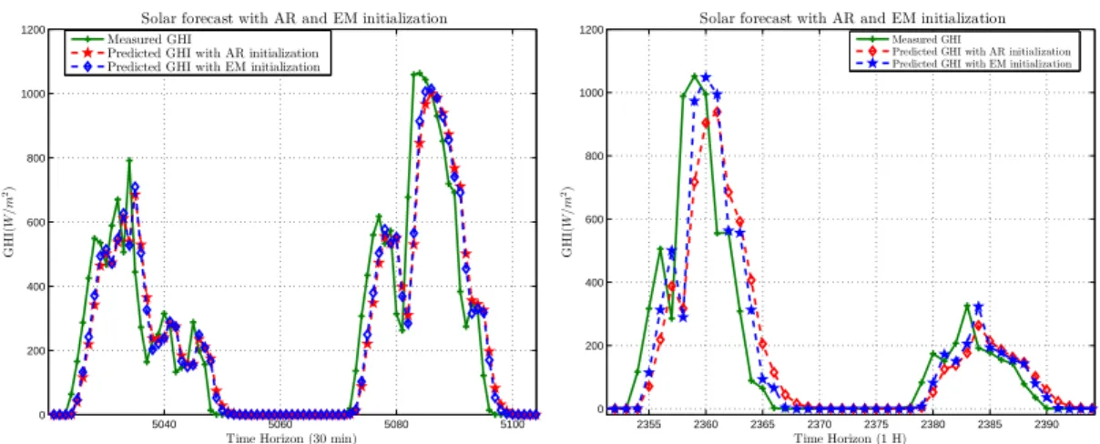
5040 5060 5080 5100 0 200 400 600 800 1000 1200
Time Horizon (30 min)
G HI ( W /m 2)
Solar forecast with AR and EM initialization Measured GHI
Predicted GHI with AR initialization Predicted GHI with EM initialization
(a) Forecast of the GHI at Time Horizon 30min. We plot on the same grpah the results obtained by the AR and EM initialization models. 2355 2360 2365 2370 2375 2380 2385 2390 0 200 400 600 800 1000 1200 Time Horizon (1 H) G HI ( W /m 2)
Solar forecast with AR and EM initialization
Measured GHI
Predicted GHI with AR initialization Predicted GHI with EM initialization
(b) Same comparison as in Figure4(a)for Time Horizon 60min.
0 200 400 600 800 1000 1200 0 200 400 600 800 1000 1200
Time Horizon (30 min)
Measured GHI Predicted GHI (W/m†) 0 200 400 600 800 1000 1200 0 200 400 600 800 1000 1200 Predicted GHI (W/m†) Time Horizon (1H)
data for AR model initialization data for EM model initialization linear FIt for EM linear Fit for AR
y(x) = a x a = 0.93315 R = 0.89609 (lin) y(x) = a x a = 0.86592 R = 0.89599 (lin) y(x) = a x a = 0.93051 R = 0.88567 (lin) y(x) = a x a = 0.91675 R = 0.88645 (lin)
(c) Real vs predicted Solar data for the AR and EM.
Figure 4. Kalman filter forecast for the Solar data (GHI) at time horizon 30min (4(a)) and 1H (4(b)). We compare the AR and EM algorithms. In graph (4(c)) we measure and compare the performance of each initialization method wrt. the fit along with a 1-st order polynomial function.
Table 2. Comparison of the different performance criterion for the different prediction models for the real Solar data (GHI) without exogenous inputs. SSpis the skill score calculated for the basic persistence model and SSspthe skill score for the smart persistence.
nRMSE (%) nMBE (%) nMAE (%) SSp(%) SSsp(%) Time Horizon
EM 7.61 0.81 3.91 7.42 6.51 1min AR 7.78 0.40 4.02 5.35 4.42 Persistence 8.22 0.00008 4.02 Smart Persistence 8.14 0.00074 3.52 EM 9.12 0.56 5.85 19.51 17.99 5min AR 9.61 0.69 6.02 15.18 13.58 Persistence 11.33 0.0006 6.96 Smart Persistence 11.12 0.0032 5.98 EM 10.22 2.68 7.37 20.40 19.15 10min AR 10.36 0.84 6.85 19.31 18.04 Persistence 12.84 0.0022 8.39 Smart Persistence 12.64 0.047 8.01 EM 11.23 4.31 9.19 31.06 30.29 30min AR 11.46 1.18 8.18 29.65 28.86 Persistence 16.29 0.0057 11.50 Smart Persistence 16.11 0.0071 11.03 EM 11.54 1.68 9.17 32.16 31.64 60min AR 12.08 1.70 9.47 28.98 28.44 Persistence 17.01 0.0057 12.46 Smart Persistence 16.88 0.0086 12.21
the maximum likelihood framework, despite the methods already presented in the literature. In addition, despite the
413
fact that there’s an important level of variability in the dataset, our methodology gives good results when accepting
414
the stationarity of the process, this assumption having as positive consequence the calibration of the filter only once
415
a time with a small amount learning dataset. All these aspects make the whole framework robust enough to perform
416
the forecasts for heterogeneous dataset for several time scales.
417
The level of performance of the approach is studied with a set of standard accuracy measures largely used in the
418
literature, named the root means square error, the mean bias error and the mean absolute error, in their normalized
419
form. We have shown that goods results of the PV forecast can be obtained by taking into consideration some
420
important exogenous variables, cloud cover and ambient temperature, that have a great influence in the production of
421
energy. In this work, these features have been used as inputs.
422
Regarding the global solar radiation forecast, the results show that our methodology outperforms by far the
clas-423
sical persistence model with a skill score improvement reaching 39.85%. They might be used as variables to be
424
estimated as we have done for the PV. Also, other variables should be incorporated in the model, as the speed of the
425
wind, to reinforce the prediction. We will address this issue soon in our research.
426
The paper tackles an important problem related to the forecast of solar and PV production. We have proposed
427
several models for parameter tuning because we believe that in high fluctuating meteorological conditions, it is not
428
obvious to build a single model which is reliable to give accurate performances for many time scales. We think that
429
it is a necessity to learn more about the variability of the solar irradiance in order to describe the whole system by a
430
set of meaningful behavioral classes. So, one could apply in parallel each model to a set of classes according to their
431
underlying characteristics. As a final benefit, the whole methodology could be implemented as a single framework
432
to do at the same time solar irradiance and PV production prediction in order to help energy provider to control and
433
manage carefully their industry.
434
References 435
[1] Akaike, H., 1971. Autoregressive model fitting for control. Annals of the Institute of Statistical Mathematics 23 (1), 163–180.
436
[2] Chaabene, M., Ammar, M. B., 2008. Neuro-fuzzy dynamic model with kalman filter to forecast irradiance and temperature for solar energy
437
systems. Renewable Energy 33 (7), 1435–1443.
438
[3] Coimbra, Carlos, F. M., Kleissl, J., Marquez, R., 2013. Solar Energy Forecasting and Resource Assessment. Elsevier, Ch. Chapter 8 Overview
439
of Solar-Forecasting Methods and a Metric for Accuracy Evaluation.
440
[4] Diagne, M., David, M., Boland, J., Schmutz, N., Lauret, P., 2014. Post-processing of solar irradiance forecasts from wrf model at reunion
441
island. Solar Energy 105, 99–108.
442
[5] Galanis, G., Louka, P., Katsafados, P., Pytharoulis, I., Kallos, G., 2006. Applications of kalman filters based on non-linear functions to
443
numerical weather predictions. In: Annales Geophysicae. Vol. 24. Copernicus GmbH, pp. 2451–2460.
444
[6] Ghahramani, Z., Hinton, G. E., 1996. Parameter estimation for linear dynamical systems. ACM Transactions on Mathematical Software
445
(TOMS) TOMS Homepage archive.
446
[7] Hassanzadeh, M., Etezadi-Amoli, M., Fadali, M, S., 2010. Practical approach for sub-hourly and hourly prediction of pv power output. In:
447
North American Power Symposium (NAPS), 2010. IEEE, pp. 1–5.
448
[8] Kailath, T., Sayed, A. H., Hassibi, B., 2000. Linear estimation. Vol. 1. Prentice Hall Upper Saddle River, NJ.
449
[9] Kalman, R. E., Bucy, R. S., 1961. New results in linear filtering and prediction theory. Journal of Fluids Engineering 83 (1), 95–108.
450
[10] Kasten, F., 1980. A simple parameterization of two pyrheliometric formulae for determining the linke turbidity factor. Meteorol. Rundsch.
451
33, 124–127.
452
[11] Kaur, A., Nonnenmacher, L., Pedro, H, T. C., Coimbra, C, F. M., ???? Benefits of solar forecasting for energy imbalance markets.
453
[12] Lorenz, E., Remund, J., M¨uller, S. C., Traunm ¨uller, W., Steinmaurer, G., Pozo, D., Ruiz-Arias, J., Fanego, V. L., Ramirez, L., Romeo, M. G.,
454
et al., 2009. Benchmarking of different approaches to forecast solar irradiance. In: 24th European photovoltaic solar energy conference,
455
Hamburg, Germany. Vol. 21. p. 25.
456
[13] Louka, P., Galanis, G., Siebert, N., Kariniotakis, G., Katsafados, P., Pytharoulis, I., Kallos, G., 2008. Improvements in wind speed forecasts
457
for wind power prediction purposes using kalman filtering. Journal of Wind Engineering and Industrial Aerodynamics 96 (12), 2348–2362.
458
[14] Mayne, D, Q., 1966. A solution of the smoothing problem for linear dynamic systems. Automatica 4 (2), 73–92.
459
[15] Ndong, J., 2014. A new approach to anomaly detection based on possibility distributions. In: INTERNET 2014, The Sixth International
460
Conference on Evolving Internet. pp. 1–8.
461
[16] Ndong, J., 2014. Using sub-optimal kalman filtering for anomaly detection in networks. Proceeding of the Electrical Engineering Computer
462
Science and Informatics 1 (1), 408–414.
463
[17] Ndong, J., Salamatian, K., 2011. A robust anomaly detection technique using combined statistical methods. In: CNSR. IEEE Computer
464
Society, pp. 101–108.
465
[18] Ndong, J., Salamatian, K., 2011. Signal processing-based anomaly detection techniques: a comparative analysis. In: INTERNET 2011, The
466
Third International Conference on Evolving Internet. pp. 32–39.
467
[19] Neumaier, A., Schneider, T., 2001. Estimation of parameters and eigenmodes of multivariate autoregressive models. ACM Transactions on
468
Mathematical Software (TOMS) TOMS Homepage archive 27 (1), 27–57.
469
[20] Pelland, S., Galanis, G., Kallos, G., 2013. Solar and photovoltaic forecasting through post-processing of the global environmental multiscale
470
numerical weather prediction model. Progress in Photovoltaics: Research and Applications 21, 284–296.
471
[21] Rabiner, L., 1989. A tutorial on hidden markov models and selected applications in speech recognition. Proceedings of the IEEE 77 (2),
472
257–286.
473
[22] Schneider, T., A., N., 2001. Algorithm 808: Arfit - a matlab package for the estimation of parameters and eigenmodes of multivariate
474
autoregressive models. ACM Transactions on Mathematical Software (TOMS) TOMS Homepage archive 27, 58–65.
475
[23] Schwarz, G., 1978. Estimating the dimension of a model. The annals of statistics 6 (2), 461–464.
476
[24] Shumway, R. H., Stoffer, D. S., 1982. An approach to time series smoothing and forecasting using the em algorithm. Journal of time series
477
analysis 3 (4), 253–264.
478
[25] Shumway, R. H., Stoffer, D. S., 1991. Dynamic linear models with switching. Journal of the American Statistical Association 86 (415),
479
763–769.
480
[26] Soubdhan, T., Emilion, R., Calif, R., 2009. Classification of daily solar radiation distributions using a mixture of dirichlet distributions. Solar
481
energy 83 (7), 1056–1063.
482