An Analytical Framework for Estimating TCO and
Exploring Data Center Design Space
Damien Hardy Marios Kleanthous Isidoros Sideris University of Cyprus Ali G. Saidi Emre Ozer ARM Yiannakis Sazeides University of Cyprus
Abstract—In this paper, we present EETCO: an estimation and exploration tool that provides qualitative assessment of data center design decisions on Total-Cost-of-Ownership (TCO) and environmental impact. It can capture the implications of many parameters including server performance, power, cost, and Mean-Time-To-Failure (MTTF). The tool includes a model for spare estimation needed to account for server failures and performance variability. The paper describes the tool model and its implementation, and presents experiments that explore tradeoffs offered by different server configurations, performance variability, MTTF, 2D vs 3D-stacked processors, and ambient temperature. These experiments reveal, for the data center configurations used in this study, several opportunities for profit and optimization in the datacenter ecosystem: (i) servers with different computing performance and power consumption merit exploration to minimize TCO and the environmental impact,(ii) performance variability is desirable if it comes with a drastic cost reduction, (iii) shorter processor MTTF is beneficial if it comes with a moderate processor cost reduction,(iv)increasing by few degrees the ambient datacenter temperature reduces the environmental impact with a minor increase in the TCO and(v) a higher cost for a 3D-stacked processor with shorter MTTF and higher power consumption can be preferred, over a conventional 2D processor, if it offers a moderate performance increase.
I. INTRODUCTION
During the last few years, datacenters have increased in numbers, size and uses [1]. In an effort to reduce costs and meet specific needs myriad configurations have come to market including micro-servers for I/O intensive workloads [2], [3] and blade-servers for space and power constrained environments. With these different systems comes a set of design decisions which effect the total cost of ownership. Consequently, to deliver a cost-efficient datacenter, designers should be aware of how different decisions affect the Total-Cost-of-Ownership (TCO) of a datacenter. Several cost models have been proposed for guiding datacenters design [4], [5], [6], [7], [8]. The following five main factors determine the TCO:
• Datacenter Infrastructure Cost: the cost of acquisition of the datacenter building (real estate and development of building) and the power distribution and cooling equipment acquisition cost. The cost of the infrastruc-ture is amortized over 10-20 years.
• Server Cost Expenses: the cost of acquiring the servers, which depreciates within 3-4 years.
• Networking Equipment Cost Expenses: the cost of ac-quiring the networking equipment, which depreciates within 4-5 years.
• Datacenter Operating Expenses: the cost of electricity for servers, networking equipment and cooling.
• Maintenance and Staff Expenses: the cost for repairs and the salaries of the personnel.
While the goal of datacenter designers is to minimize the TCO, another major concern is the energy consumption and the resulting environmental impact of such IT infrastructures. The
CO2 footprint is directly linked to the energy consumption, which corresponds to a substantial fraction of the TCO.
Research and commercial efforts are underway to re-duce the energy consumption by choosing low-power based servers [9], [2], by reducing the server idle consumption [10] or by reducing the cooling power [11], which represents a significant part of the Power Usage Effectiveness (PUE) [12]. Also, an attempt is observed to reduce datacenters energy by optimizing their utilization with virtualization or more efficient co-location [13], [14], [15].
These trends render essential tools to assess the benefits and drawbacks of datacenter design choices on the TCO and the environmental impact. Only few tools, to the best of our knowledge, are publicly available to calculate TCO and these do not allow easy user exploration and fined grain design choices. APC [16] provides an online estimator tool while [7], [17] provide spreadsheets to estimate the TCO. Nevertheless, these tools provide the basic parameters and the framework that our tool is based on. Other studies [18], [19], [20], [21], [22], [23] have developed their in-house model to assess the impact of their design solution on the TCO. Companies like Facebook or Google, it is virtually certain, have their own models but they are unlikely to release their tools. Our publicly available tool1can offer a common framework for future research in this
area and it can be combined with datacenter simulation tools [24] to enable more accurate exploration of datacenter design choices.
In this paper, we present EETCO: an estimation and exploration tool to provide qualitative trends of datacenter design decisions on TCO and environmental impact. This tool enables the exploration of the implications of several data center parameters including server performance, power, cost and mean-time-to-failure (MTTF). The tool also includes a model that estimates the cold spares needed due to server failures and the hot spares needed to compensate servers performance variability. More details on the hot and cold spares are given in Sections II and III.
The tool takes as inputs coarse and fine grain data center design parameters like PUE, racks organization, components cost, power consumption and MTTF, and produces outputs
related to the organization and operation of a datacenter. The tool contains a kernel estimation component that is used by wrappers to explore design decision tradeoffs on TCO, which can reveal opportunities and challenges for the different parts of the datacenter ecosystem (hardware manufacturer, hardware vendor, datacenter designer).
In the experimental section of the paper, wrappers are defined to explore high-performance vs. low-power based servers as well as the implications of performance variability, varying MTTF, changing ambient temperature and 2D vs 3D-stacked processors. These experiments reveal the conditions under which servers with different computing performance, power, cost and MTTF provide opportunity to reduce either or both the TCO and theCO2 footprint.
The remainder of the paper is organized as follows. Sec-tion II overviews the proposed framework, while model details are given in Section III. The validation and experimental results are given in Section IV. Section V discusses the implementa-tion and future extensions and Secimplementa-tion VI concludes the paper.
II. FRAMEWORK OVERVIEW
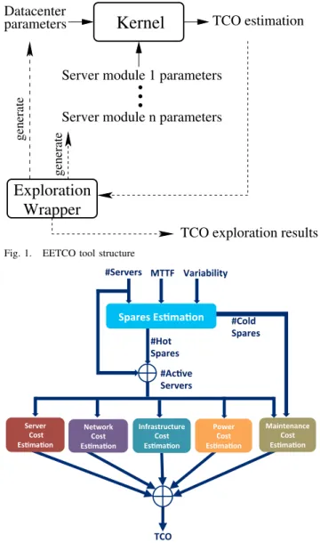
Our tool is built in two parts as illustrated in Figure 1. The first one is the kernel of the tool, which takes as inputs a dat-acenter configuration (land/building acquisition cost, cooling equipment cost per Watt) and configurations for different types of server modules (rack configurations, DRAM, processor and other components cost/power/MTTF).
The kernel produces the TCO and environmental impact estimation and other outputs related with the organization and operation of a datacenter (the five main factors of the TCO for the whole datacenter and per resource, the datacenter area, the number of racks, the total power consumption, for a rack the per resource total power consumption).
The second part, illustrated by the exploration wrapper, corresponds to a specific wrapper, which generates datacenter and server modules configurations for design space explo-ration, maintains the kernel’s results for each configuration evaluated and returns the overall results. Different wrappers can be defined according to trade offs the user wants to explore. For instance, in the experimental results section, wrappers are defined to compare high-performance vs. low-power based servers and to investigate the effects of changing ambient temperature.
One wrapper, we would like to highlight, has the ability to produce what should be the value for a given input parameter, such as MTTF, while sweeping through a range of values for another input parameter, such as performance, to maintain constant a given output parameter, such as TCO. This wrapper helps produce a curve that divides a two dimensional explo-ration space into a region where the output parameter increases and another where it decreases, as compared to a reference design point. For example, using this wrapper someone can explore the design of a datacenter with different server types and decide what will be the best mix for their workload requirements.
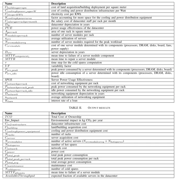
An overview of the kernel framework is shown in Figure 2 and detailed in the next section. For each different server configuration type (compute nodes, database nodes, storage nodes), the estimation starts with spares estimation that deter-mines (i) the number of hot spares required to mitigate perfor-mance variability and ensure meeting perforperfor-mance requirement for the peak workload, and (ii) the number of cold spares
Fig. 1. EETCO tool structure
Fig. 2. Kernel framework overview
needed due to server failures. The number of active servers, initial number of servers estimated assuming no variability plus the hot spares, will determine the costs for datacenter infrastructure, server acquisition, networking equipment, and power. The cold spares are used to determine the maintenance cost. These costs are then summed together to produce the contribution to the TCO of a given server type. The global TCO is the sum of the contribution from all server types.
III. TCOESTIMATION
As shown in the previous section, the TCO estimation is the sum of the datacenter infrastructure cost (Cinf rastructure),
the server acquisition cost (Cserver), the networking equipment
cost (Cnetwork), the power cost (Cpower) and the maintenance
cost (Cmaintenance).
T CO=Cinf rastructure+Cserver+Cnetwork (1)
+Cpower+Cmaintenance
In the above formula, the first line represents the capital expenses (CAPEX) and the second represents the operational expenses (OPEX).
In this section, we present the model used to determine these different factors. The list of input parameters and output
results is shown in Tables I and II according to the following notation:
• N denotesNUMBER(e.g. number of required server modules, number of spares etc)
• C denotesCOST (e.g. server module cost, electricity cost etc)
• A denotesAREA(e.g. datacenter area, cooling equip-ment area, etc)
• K denotes aRATIO(e.g. server modules per rack etc) • P denotes POWER(e.g. total server power etc) • D denotesDEPRECIATION(e.g. server, data center) The resulting TCO with multiple server configurations can be easily determined under the assumption that, the contribu-tion of each server configuracontribu-tioniis additive:
T CO=X i Cinf rastructure,i+ X i Cserver,i (2) +X i Cnetwork,i+ X i Cpower,i+ X i Cmaintenance,i
Without loss of generality and for ease of reading, a single server configuration is assumed in the following formulas.
In the next subsections, the different computation steps of the model estimation are described according to the flow in Figure 2, starting with spares estimation followed by the various cost estimations.
A. Hot and cold spares estimation
The distinction between hot and cold spares nodes is nec-essary, since the hot spares have to be accounted in the power consumption, the cooling and power distribution requirements, whereas, the cold spares are only accounted in the maintenance cost.
1) Hot spares estimation: Various technological, opera-tional and environmental conditions [25] can lead to processor performance variations. That is, in a population of processors, some of them are expected to be affected by a medium/high performance degradation while others will not be affected at all. This performance variation determines the need for hot spares to compensate the performance degradation. For in-stance, if the expected performance is at 90% of the maximum and the workload requirements are 10000x throughput (e.g. 10000 cores running separate threads), then we will need (10000/0.9 - 10000) 1111 extra cores to meet our require-ments, which translates to extra server costs for acquisition, maintenance, power consumption and space.
To consider the performance variation, avariability factor (VF) is introduced. VF takes values from 0 to 1, with 0 meaning no degradation at all and 1 means no operation. The performance is thus given by 1−V F. With this factor, the number of hot spares is determined as follows:
Nhotspares=
Nsrvmodulesreq
1−V F −Nsrvmodulesreq where Nsrvmodulesreq is the number of server modules
re-quired for the peak workload when VF=0.
In the following, the notation Nsrvmodules represents the
number of active servers that is equal to the sum ofNhotspares
andNsrvmodulesreq modules.
2) Cold spares estimation: Cold spares are server modules needed for replacement when active servers failed. The fault rate of a server can be determined by the MTTF of its components. By assuming a constant fault rate, an exponential
distribution can be used to determine the number of cold spares required at a given timetas follows:
Ncoldspares(t) =
Nsrvmodules Dt −
Nsrvmodules
whereDt is defined as follows: Dt=e
−t M T T Fallunits
According to the exponential distribution, the total MTTF of a server module is obtained using the MTTFs of the components:
M T T Fallunits= 1 P i 1 M T T Fcomponenti
In the equations above we assume that the server modules with a failure in any component are replaced.
FormulaNcoldspares(t), assumes that all the replacements
are performed at the end of the intervalt, which is not accurate. To be more accurate, we can estimate the required cold spare modules in the interval [0,t] by partitioning it in k adequately short time intervals of τ duration (t = kτ), and account for different amount of aging for the newly replaced at the end of each such interval.
By definition, the number of server modules needed for replacement at time 0 is equal to 0 (CS0 = 0) and after the short time intervalτ this number is given by:
CSτ =Nsrvmodules∗( 1
Dτ −
1)
Normally, the number of spares for the time interval [0,2τ]
would be obtained as for the[0, τ], but since the modules have different age: theCSτ modules, replaced at timeτ, will have
ageτ and the rest (Nsrvmodules−CSτ) will have age2τ, we
have the following formula:
CS2τ= CSτ−CS0
Dτ +
Nsrvmodules
−CSτ
D2τ −Nsrvmodules
And after the elapse of the interval[0, kτ]the required number of cold spares is given by:
CSkτ =h k−1 X i=1 CS(k −i)τ−CS(k−i−1)τ Diτ i (3) +Nsrvmodules−CS(k−1)τ Dkτ −Nsrvmodules
By considering kτ equal to the server depreciation, we obtain the number of cold spares, noted hereafterNcoldspares,
that are considered in the maintenance estimation cost. If we have all the cold spares timely available, then the expected fraction of the servers (or Available Throughput) that are available at any given time will be:
AvailableT hroughput= 1
1 +CSkτ∗M T T R/(24∗365)
Nsrvmodules∗Dsrv where M T T Ris the mean time to repair a server module in hours (i.e. the mean time needed to replace it) andDsrvis the
server depreciation in years.
B. Cost and environmental impact estimation
The different costs are simply derived from the number of server modules and number of cold spares as explained next. 1) Maintenance Cost: The maintenance cost per month is determined as follows:
Cmaintenance=
Ncoldspares∗Csrvmodule
Dsrv∗12 (4)
+Nracks∗Csalaryperrackpermonth
where Csrvmodule is the cost of one server module, Csalaryperrackpermonthis the salary cost of datacenter staff per
TABLE I. INPUT PARAMETERS
Name Description
Cbuildingpersqm cost of land acquisition/building deployment per square meter
Ccooling&power eqperW cost of cooling and power distribution infrastructure per Watt
CelecperKW h electricity cost per KWh
Kcooling&powerarea factor accounting for more space for the cooling and power distribution equipment
Csalaryperrackpermonth the salary cost of datacenter staff per rack per month
Ddc datacenter depreciation in years
P U E power usage effectiveness of the datacenter
Aperrack area of one rack in square meter
Kmodulesperrack number of server modules per rack
usrv average utilization of servers
Nsrvmodulesreq number of server modules required for the peak workload
Csrvmodule cost of one server module determined with its components (processors, DRAM, disks, board, fans,
power supply)
Dsrv server depreciation in years
M T T Fcomponenti mean time to failure of a server module component
M T T R mean time to repair a server module
τ time step for the cold spares computation
V F variability factor
Psrv peak peak power consumed by a server determined with its components (processors, DRAM, disks, board)
Psrv idle power idle consumption of a server determined with its components (processors, DRAM, disks,
board)
SPUE Server Power Usage Effectiveness
Cnetworkperrack cost of networking equipment per rack
Pnetworkperrack peak peak power consumed by the networking equipment per rack
Pnetworkperrack idle idle power consumed by the networking equipment per rack
Dnetwork networking equipment depreciation in years
unetwork average utilization of networking equipment
Kloan interest rate of a loan
TABLE II. OUTPUT RESULTS
Name Description
T CO Total Cost of Ownership
Env Impact Environmental impact in kg CO2per year
Cinf rastructure datacenter infrastructure cost
Cbuilding land/building acquisition cost
Ccooling&power equipment cooling and power distribution equipment cost
Nracks number of racks
Cserver server acquisition cost
Nsrvmodules number of active servers (Nsrvmodulesreq+Nhotspares)
Nhotspares number of hot spares
Cnetwork network cost
Cpower power cost
Ptotal peak total peak power consumption
Ptotal peak perrack total peak power consumption per rack
Ptotal avg total average power consumption
Cmaintenance maintenance cost
Ncoldspares number of cold spares
M T T Fallunits mean time to failure of a server module
AvailableT hroughput expected fraction of available servers in the datacenter
as follows:
Nracks=
Nsrvmodules Kmodulesperrack
where Kmodulesperrack is the number of server modules per
rack.
2) Networking Cost: The networking acquisition cost per month is determined as follows:
Cnetwork=
Nracks∗Cnetworkperrack Dnetwork∗12
where Dnetwork is the networking equipment depreciation in
years and Cnetworkperrack is the networking equipment cost
per rack. This cost account for the networking gear at the edge, aggregation, and core layers of the datacenter and assume that the cost scales linear with the number of racks.
3) Server Cost: The server acquisition cost per month is determined as follows:
Cserver=
Nsrvmodules∗Csrvmodule Dsrv∗12
More details for the server components are given in Table I. 4) Power Cost: The power cost per month is determined as follows:
Cpower =P U E∗ CelecperKW h∗30∗24
1000 (5)
∗(SP U E∗Ptotal srv+Ptotal network)
where P U E is the power usage effectiveness of the dat-acenter (the ratio of total power of the datdat-acenter to the IT power),SP U E [12] is the Server Power Usage Effectiveness (The ratio of total power of a server to the power of pure electronic components) andCelecperKW his the electricity cost
per KWh. Ptotal srv is the total power consumption of all
the active servers considered in the power cost estimation. Depending on how the service provider is charged for the energy they consumed [26]: the peak power consumption or the actual consumption, the peak power (Ptotal srv peak) or
the average power (Ptotal srv avg) has to be used. Ptotal srv peak=Nsrvmodules∗Psrv peak
Ptotal srv avg=Nsrvmodules (6)
∗(usrv∗Psrv peak+ (1−usrv)∗Psrv idle)
wherePsrv peak is the peak power consumed by a server, Psrv idle is the power idle consumption of a server andusrv
is the average server utilization. An interesting direction for future work is extending the tool by modeling a more dynamic load behavior.
Finally, Ptotal network is the total power
consump-tion of the networking equipment and can be com-puted in a similar manner by replacing Nsrvmodules by Nracks,usrv by unetwork,Psrv peak byPnetworkperrack peak
and Pnetworkperrack idle to obtain Ptotal network peak and Ptotal network avg.
5) Infrastructure: The datacenter infrastructure cost per month is determined as follows:
Cinf rastructure=
Cbuilding+Ccooling&power equipment Ddc∗12
where Cbuilding is the land/building acquisition cost, Ccooling&power equipmentis the cooling and power distribution
equipment cost andDdcis the datacenter depreciation in years. Cbuilding=Aperrack∗Nracks (7)
∗Kcooling&powerarea∗Cbuildingpersqm
whereAperrackis the area of one rack,Kcooling&powerarea
is a factor accounting for more space for the cooling and power distribution equipment andCbuildingpersqmis the cost of land
acquisition/building deployment per square meter.
Ccooling&power equipment=Ccooling&power eqperW (8)
∗(Ptotal srv peak+Ptotal network peak)
where Ccooling&power eqperW is the cost of cooling and
power distribution infrastructure per Watt.
6) Impact of Loan Interest: CAPEX are usually subject to loans based on an interest rate and a constant payment schedule. This cost is determined as follows:
C∗Kloan12
1−(1 + Kloan12 )(−D∗12)
whereCrepresents each of the CAPEX (infrastructure, servers and networking equipment) cost over their depreciation period
DandKloanis the interest rate.
7) Environmental impact estimation: A conversion fac-tor [27] can be used to translate the actual power consumption into the emission of CO2 in kg. Thus, the environmental impact per year can be estimated as follows:
Ptotal avg∗P U E∗24∗365
1000 ∗0.54522
where
Ptotal avg=Ptotal srv avg∗SP U E+Ptotal network avg
IV. VALIDATION ANDCASE STUDIES
In this section we first validate the EETCO model (IV-A), and then we describe the experimental assumptions (IV-B),
TABLE III. EETCO MODELVALIDATION
TCO Component % of TCO in [17] % EETCO model Difference
Cinf rastructure 22% ($763,672) 21% ($763,707) +0.04%
Cserver 57% ($1,998,097) 57% ($1,998,102) 0.1%
Cnetwork 8% ($294,943) 8% ($295,081) -0.16%
Cpower 13% ($474,208) 13% ($473,784) 0.02%
Cmaintenance - -
-TCO Component % of TCO in [12] % EETCO model Difference
Cinf rastructure 14% 12% -2%
Cserver 70% 72% +2%
Cnetwork - -
-Cpower 7% 7% 0%
Cmaintenance 9% 9% 0%
and use our validated model to present and analyze the experimental results (IV-C). The results include some case studies that reveal opportunities and challenges for different segments of the datacenter ecosystem.
A. Model validation
The model used in the proposed tool is validated by com-paring its TCO breakdown against two previously published TCO breakdowns of large-scale data centers [17], [12]. The comparison is shown in Table III. For both comparisons, we use data center configurations as close as possible to the ones used in the previous studies. Our tool models the infrastucture, server, network, power and maintenance cost while Barosso et. al does not model the network cost and Hamilton does not model the maintenance cost. As such, when comparing our model to theirs we cannot compare with the missing data. The results of these comparisons show that our model produces similar breakdown and, therefore, increases our confidence about its accuracy.
The comparison against [17] using absolute values, shown in Table III, is also very accurate. In [12] the breakdown is only provided as percentage and, therefore, we could not assess the accuracy of the proposed model against absolute values. B. Experimental setup
The experiments are conducted using two different server configurations named LPO and HPE. LPO represents a Low-Power High-Density server configuration, based on low-power ARM/Atom processors [2], [3], while HPE represents a High-Performance server configuration based on high-performance Intel Xeon like processors. For the HPE server we consider 12GB DRAM and 2 disks on a dual socket motherboard in a 1U blade [28]. For the LPO server we consider 48 chips split on 12 motherboards (each motherboard with 16GB DRAM and 2 disks) in a 2U blade[29]. The decision of the DRAM capacity was based on the assumption that each core will be allocated 1GB of DRAM (LPO is based on a 4 core processor and HPE is based on a 6 core processor).
Tables IV, V and VI provide the breakdown of the cost and power consumption for both configurations and their common characteristics. For LPO, SPUE is assumed to be 1.1 to take into account the cooling cost reduction of the low-power configuration as compared to HPE (SPUE = 1.2). The power contribution of the power supply and fans for both configuration is directly determined in EETCO with SPUE and presented here for completeness.
For each experiment, unless noted otherwise, 50000 servers are assumed and the peak power consumption (noted peak) and the actual power consumption (noted average) is used to compute the power cost, when it makes a difference. Also we would like to note that the maintenance model assumes that the
TABLE IV. HPE 1UBLADE SERVER CONFIGURATION. Components Cost Power Power
($) (W) idle (W)
2 Processors 2200 190 60 12 GB DRAM 300 6 1.5 2 Disks 360 20 10 Power supply, 900 43.2 14.3 board and fans
Total 3760 259.2 85.8
TABLE V. LPO 2UBLADE SERVER CONFIGURATION.
Components Cost Power Power
($) (W) idle (W)
48 Processors 4800 144 24 192 GB DRAM 4800 96 24 24 Disks 1200 240 120 Power supply, 1380 48 16.8 board and fans
Total 12180 528 184.8 TABLE VI. COMMON SERVER CONFIGURATION
Parameter Value
usrv 0.2
Dsrv 3 years
τ 1 day
V F 0
TABLE VII. DATACENTERCONFIGURATION
Parameter Value
Cbuildingpersqm 3000$/m2
Ccooling&power eqperW 12.5$/W
CelecperKW h 0.07$
Kcoolingarea 1.2
Csalaryperrackpermonth 200$
Ddc 15 years
PUE 1.3 (HPE), 1.2 (LPO) TABLE VIII. RACK AND NETWORK CONFIGURATIONS
parameter value
Rack 42U
Aperrack 1.44m2(with: 0.6m ; depth 1.2m ; used distance 1.2m)
Kmodulesperrack LPO: 252 (21 blades per rack ; 12 servers per 2U blade)
HPE: 42 (42 blades per rack ; 1 server per 1U blade)
Cnetworkperrack 10K$
Pnetworkperrack peak 360W
unetwork 1
Dnetwork 4 years
Fig. 3. TCO sensitivity analysis of HPE configuration
total blades MTTF is not affected on a failure and replacement of a server module. That means that in case of a server module failure, only that module will need to be replaced and not the whole blade.
Tables VII and VIII summarize the datacenter, the rack and network configurations. At the rack level, the LPO configura-tion contains 21 2U blade servers while the HPE configuraconfigura-tion contains 42 1U blade servers.
We use publicly available data from published papers and industrial data to select representative values for the various parameters: [12], [7], [30], [17], [31], [5], [4] for the data-center configuration, [32], [12], [17] for the common server configuration, and [29], [3], [33], [34], [10], [35], [18], [36] for the server configurations.
The M T T Fallunits is computed assuming 100 years
MTTF [35] per disk, 200 years MTTF [34] per 4GB DRAM DIMM. For processors the reported MTTF varies from 30 years [37] to 100 years [35]. We use 30 years for HPE processor and 100 years for LPO processor to account for their difference in term of chip size and thermal behavior. The resultingM T T Fallunitsis 9.836 years and 12.5 years for HPE
and LPO respectively.
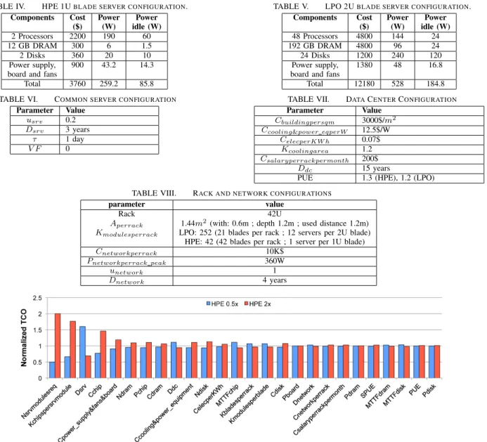
A sensitivity analysis is performed on the baseline HPE configuration to show how changing the different parameters affects TCO. The baseline values are shown in Tables IV -VIII for the HPE server. In Figure 3, we show the sensitivity of the TCO value by halving (0.5x) and doubling (2x) the baseline value. Only parameters with an impact higher than 1% are shown and the parameters are sorted from high to low sensitivity. The Figure shows parameters that determine the server organization (processors, DRAM, disk) exhibit the largest sensitivity. This is explained by the large contribution of server cost to TCO (more than 50%). The results for the LPO configuration are almost identical (not shown for clarity). In the next section we present analysis of various compar-isons and case studies: the TCO breakdown of the HPE and LPO server configurations, the significance of more accurate cold spares estimation, the impact of performance, power, cost and MTTF, the effect of performance variation, the implications of ambient temperature on the TCO and the environment and an initial analysis of the potential benefits of 3D integration.
Fig. 4. Breakdown of LPO and HPE configurations
C. Experimental results
TCO Breakdown for LPO and HPE: The TCO break-down of a datacenter populated with LPO and HPE server configurations is shown in Figure 4. The average power cost is normalized with the peak power cost for each server configuration respectively.
As shown in the Figure, the server cost represents the most important part of the TCO, 69% and 57% for each configuration followed by the maintenance cost (18% LPO and 20% HPE). The power cost differs when the peak and the average is assumed. For the peak power consumption (the sum of peak and average in the figure), the resulting cost is 6% for LPO and 10% for HPE while, when the average is assumed, a saving of 3% and 5% for LPO and HPE respectively is observed. This difference in power is explained by considering the ratio of power consumption and the power consumption at idle time, which is more significant for the HPE configuration. The direct TCO comparison across the two server con-figurations is meaningless since the two concon-figurations may have different performance. An exploration that considers the performance impact across configurations is performed subsequently.
Benefits of the cold spares estimation model: The benefits of more precise cold spare estimation are shown in Figure 5 for different time stepsτ.
As shown in the Figure, considering that at any given time not all modules have the same age can reduce significantly the estimated number of cold spares (up to 14% for LPO and 19% for HPE) and consequently the maintenance cost (up to 13% for LPO and 16% for HPE). For example, if we consider the interval for cold spare estimation for the HPE to be 1 year (τ
= 365) this will lead to 5.1% more cold spares that correspond to 4.5% increase in the maintenance cost estimation.
We have also examined the benefit of values smaller than
τ = 1 day and the results showed minor improvement in precision. So, we considerτ = 1 day as the smallest interval for cold spare estimation.
Impact of the processor’s MTTF: Attempting to improve a processor’s MTTF may increase its cost due to the use of more expensive and reliable components. In this experiment, the trade-off between the processor’s MTTF and the processor’s cost is explored. The selected range for processor’s MTTF is 20 to 150 years which examine the trends near the range reported in previous work [37], [35].
Figure 6 shows what should be the processor’s cost to keep the TCO constant when the MTTF varies relative to a reference value (30 and 100 years for HPE and LPO respectively, shown with the black dots in the figure).
As shown in the figure, for the HPE configuration, an in-crease (up to 2x) in terms of MTTF budget may be interesting.
Fig. 5. Impact of time step τ on the #coldspares (dash line) and the maintenance cost for LPO and HPE. Results are normalized withτ = 1
day
Fig. 6. Impact of processor’s MTTF. Results normalized with those obtained with the reference value
For 2x MTTF, a price increase near 20% is affordable, while above this region the price cost stays nearly constant. The LPO can benefit by decreasing the MTTF, but the processor cost reduction has to be significant when the MTTF is below2/3
(66 years) of the reference value. Smaller changes of MTTF, in both directions, require moderate changes in the cost.
These observations are interesting for: (i)processor man-ufacturers to assess how the MTTF of processor affects the TCO and to estimate the potential profit for a given design and MTTF budget; (ii) hardware vendors to increase their margin by selecting the appropriate processor;(iii)datacenter designers to reduce the TCO when they have the choice between processors with equivalent performance but different prices and MTTF, and to define their maintenance model.
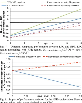
Different computing performance between servers: The TCO breakdown is not sufficient to compare the two server configurations since they may not have the same computing performance. Let us assume that LPO server configuration will require more processors to reach the same computing perfor-mance as HPE. We use an equivalent perforperfor-mance coefficient (epc), defined to be how many LPO processors are required to reach the computing performance of one HPE processor. We vary epc from 1 to 6, which is a representative range across servers with different processors for cloud applications derived from [38], to observe the trends. Results are presented in Figure 7 and the values are normalized with the TCO and the environmental impact obtained with HPE.
As shown in the Figure, when epc is relatively small, the TCO obtained with the low-power configuration (LPO) is better. At a given point (epc ∼ 3.5 in our case for 1GB per core of DRAM) the TCO of both configurations is equal. Nevertheless, in that case the resulting environmental impact is
Fig. 7. Different computing performance between LPO and HPE. LPO results normalized with HPE results.Nsrvmodulesreq(LP O) = epc∗
Nsrvmodulesreq(HP E)
Fig. 8. Impact of performance variation for the HPE configuration. Results are normalized with those obtained when VF=0
lower with LPO. LPO is, thus, preferable for the environment for equivalent TCO. After that point, HPE is a better choice for both the TCO and the environmental impact. The results also indicate that when the total datacenter’s DRAM is kept equal for both configuration the benefits of the LPO server is higher. Awareness of such trends can be useful: (i) for processor manufacturers to design processors that can trade-off between performance and cost and(ii)for datacenter designers to optimize for both the TCO and CO2.
Impact of performance variation: As mentioned in the previous section, there are various sources of processor per-formance variability. This variation may affect the processor’s cost in addition to performance [39] (i.e. the higher the variation, the lower the processor’s cost). In this experiment, a variability factor (VF) is assumed to range from 0 to 0.1 while power remains unchanged. The results, illustrated in Figure 8, show what should be the processor’s cost to keep the TCO constant. The figure also show the environmental impact of performance variability.
As shown in the figure, if the processor’s cost reduction is higher than the reduction needed to keep the TCO constant (i.e. below the iso curve), there is an opportunity to reduce the TCO. This positive impact of performance variability comes at the price of an environmental impact increase. In fact, the higher the performance variability, the higher the number of active servers needed, which results inevitably in a higher energy consumption and thus higher CO2 emissions.
This data presents: (i) for processor manufacturers an opportunity to sell (or even design) processor with performance variability instead of throwing away processors with high variability. A key challenge is the design processors with performance guarantees and with less power consumption in case of variability (by disabling units for instance);(ii)for the hardware vendors a challenge to define business models to deal
Fig. 9. Impact of temperature. Results are normalized with those obtained when T=20◦C
Fig. 10. 2D vs. 3D processor. Results are normalized with those obtained with LPO configuration
Fig. 11. 3D processor’s design space exploration of MTTF and cost
with performance variability;(iii)for datacenter designers an opportunity to reduce the TCO.
Impact of ambient temperature: This experiment addresses the effect of ambient temperature (assumed 20◦C) on the
TCO and the CO2 emissions. An increase in the ambient temperature from 20◦C to 30◦C has a positive impact on
the cooling power consumption (in a previous study the PUE scales from 2 to 1.65 [40]) while the MTTF is reduced [40], [41]. In this experiment, we assess this positive and negative impact by assuming a linear reduction of the PUE per degree and a constant server’s power consumption. We also use the same values for PUE and ambient temperature as in [40].
Moreover, the effect of the ambient temperature on the MTTF is model by the Arrhenius equation to predict the acceleration factor (AF) due to the temperature:
AF =eEak (Tr1−Ta1 )
whereEais the activation energy in electron-volts (0.3 in our case), k is the Boltzmanns constant (8.617E-05),Tr and Ta are the reference temperature (20◦C + 273) and the actual
temperature, in degrees Kelvin.
temperature can be determined as follows:
M T T F = M T T Fref
AF
whereM T T Fref is theM T T F at the reference temperature.
As shown in Figure 9, the CO2 emissions is significantly reduced while we can observe a small TCO increase (HPE and LPO TCO average lines overlap). Consequently, increasing by few degrees the ambient datacenter temperature appears to be a good trade-off to reduce the environmental impact without increasing significantly the TCO.
Comparison between 2D and 3D processors: To overcome the memory wall, 3D-stacking architectures have received significant attention by the architecture community [42], [43], [9], [44] in the last few years to improve performance by stacking multiple DRAM layers on top of a logic layer. This approach provides higher performance as compared to 2D processors but with the trade-off of (i) higher processor cost and processor power consumption, (ii)chip temperature increase and(iii)probably a lower MTTF due to the stacking of multiple layers.
In this experiment, we try to assess the overall benefits of 3D-stacked chips as compared to 2D processors. To the best of our knowledge, this is the first time such a comparison is performed with the datacenter TCO perspective in mind. The basic idea behind a 3D chip design is that the increased performance and reduced overall server power due to the 3D-integrated DRAM will cover the extra cost of stacking 3D chips and possible reduction in the MTTF.
For the 3D server configuration we use the LPO config-uration as baseline with the difference that the 4GB off-chip DRAM per chip is now integrated with the 3D chip. In Fig-ure 10 we attempt to project what should be the performance increase for tolerating the cost and power increase to keep the TCO constant equal to the LPO datacenter configuration.
The 3D chip cost increase is due to the 3D stacking process and the 3D-integrated DRAM and the power increase is due to the additional power of the 3D-integrated DRAM, assuming that the off-chip DRAM interface is still maintained. For example let’s assume that a 3D chip cost will be at least the cost of the LPO chip ($100) + the cost of the DRAM ($100) + a cost for 3D stacking, testing and packing, extra provisions for MTTF and possible additional cooling solutions (35% increase) that equals to a minimum price of $270. Also let’s assume that the 3D-integrated DRAM has lower power, 1 Watt, as compared to the off-chip DRAM (2 Watt). That makes the total power of the 3D chip equal to the LPO chip power (3 Watts) + the 3D-integrated DRAM (1 Watt) = 4 Watts. The overall power for the 3D chip based servers will decrease because we replace the 2 Watt off chip DRAM with the 1 Watt 3D-integrated DRAM.
As shown in Figure 10, the performance increase should be at least 1.2X to have enough room (below the curve) to support the cost and power consumption increases due to 3D stacking and to improve the Performance/TCO. Also, Figure 10 reveals that the cost can be increased up to 200% when the power stays the same and the power increase up to 500% when the server cost stays constant and with the same performance.
Another possible design space exploration is the trade-off between the 3D chip’s MTTF and its cost. Figure 11 shows the iso curve of the MTTF reduction over the processor’s cost increase for a constant TCO. The figure also shows that the
relation between MTTF and processor’s cost is due to the increase of cold spares needed with lower MTTF. For this experiment, we assumed that the 3D chip can achieve a 1.2X performance improvement with 4 Watts power consumption. The processor’s cost is normalized to $200 which we assume to be the minimum cost for the logic and 3D-integrated DRAM dies and the processor’s MTTF is normalized to the combined MTTF of the LPO chip (100 years) and the DRAM DIMM (200 years) which equals to 66.7 years.
The results in Figure 11 indicate that if the 3D chip can provide the maximum MTTF, which is the combined of the two components, then we can spend up to 40% more from the initial cost ($200) on the 3D stacking process. Another observation is that a 35% for 3D stacking process can be afforded as long as the combined MTTF does not drop below 80% of the ideal. This can motivate a company producing 3D chips to invest that amount to improve their 3D stacking process and target a combined MTTF of 80% of the ideal which will result to the same TCO as a 2D-chip LPO server based datacenter.
This initial comparison of 2D and 3D processors, from a datacenter TCO perspective, shows interesting trends that motivates examining the trade-offs between performance, cost, power and MTTF for profitable 3D processor deployment in servers for datacenters. This experiment merits to be explored in more detail with more precise models for MTTF, thermal, power consumption and 3D processors cost and performance which is part of our ongoing work.
V. FUTURE EXTENSIONS
In its current version, the tool has the ability to provide qualitative trends about datacenter design decisions and we believe that this tool will be useful for different research communities to explore trade offs at different levels of the datacenter ecosystem.
The EETCO tool is implemented in Perl in an object oriented manner to allow flexibility and easy extensions. The plans for future extensions to the TCO tool are:
• different hardware maintenance models
• a model for the virtual machine, software and the software maintenance contributions to the TCO • a model at the service level based on different kind of
server configurations and utilization
• validation of our model with data coming from avail-able information on datacenters
• federated data centers, consider TCO trade-offs of using different number of facilities and locations • combine EETCO tool with a datacenter load
simula-tion tool.
VI. CONCLUSION
In this paper, we have presented EETCO: an estimation and exploration tool that provides qualitative trends of datacenter design decisions on TCO and environmental impact. The tool model considers many of the key datacenter parameters and is shown to be quite accurate against previous published TCO breakdown. Different case studies have been performed to assess tradeoffs, among other, between server configurations, performance variability, datacenter ambient temperature, and 3D processor integration.
This reveals opportunities and challenges for how to tune and optimize the datacenter ecosystem. As future work, we plan to extend the tool in different directions including hetero-geneous processor modeling and federated datacenters.
ACKNOWLEDGMENT
The research leading to this paper is supported by the European Commission FP7 project ”Energy-conscious 3D Server-on-Chip for Green Cloud Services (Project No:247779 ”EuroCloud”)”.
REFERENCES
[1] Cisco, “Cisco global cloud index: Forecast and methodology, 20112016,” 2012.
[2] Calxeda, “http://www.calxeda.com.” [3] seamicro, “http://www.seamicro.com/.”
[4] C. Patel and A. Shah, “Cost model for planning, development and operation of a data center,” HP Laboratories Palo Alto, Tech. Rep., 2005.
[5] J. Karidis, J. E. Moreira, and J. Moreno, “True value: assessing and optimizing the cost of computing at the data center level,” in
Proceedings of the 6th ACM conference on Computing frontiers, ser. CF ’09. New York, NY, USA: ACM, 2009, pp. 185–192.
[6] J. Moore, J. Chase, P. Ranganathan, and R. Sharma, “Making scheduling ”cool”: temperature-aware workload placement in data centers,” in
Proceedings of the annual conference on USENIX Annual Technical Conference, ser. ATEC ’05. Berkeley, CA, USA: USENIX Association, 2005, pp. 5–5.
[7] J. Koomey, K. Brill, P. Turner, J. Stanley, and B. Taylor, “A simple model for determining true total cost of ownership for data centers,” white paper, Uptime Institute, 2007.
[8] K. V. Vishwanath, A. Greenberg, and D. A. Reed, “Modular data centers: how to design them?” inProceedings of the 1st ACM workshop on Large-Scale system and application performance, ser. LSAP ’09. New York, NY, USA: ACM, 2009, pp. 3–10.
[9] E. Ozer and et al., “Eurocloud: Energy-conscious 3d server-on-chip for green cloud services,” in2nd Workshop on Architectural Concerns in Large Datacenters, 2010.
[10] D. Meisner, B. T. Gold, and T. F. Wenisch, “Powernap: eliminating server idle power,” inProceeding of the 14th international conference on Architectural support for programming languages and operating systems, ser. ASPLOS ’09. New York, NY, USA: ACM, 2009, pp. 205–216.
[11] N. El-Sayed, I. Stefanovici, G. Amvrosiadis, and A. A. Hwang, “Tem-perature management in data centers: Why some (might) like it hot,” inProceedings of SIGMETRICS 2012, 2012.
[12] L. A. Barroso and U. Holzle, “The datacenter as a computer: An introduction to the design of warehouse-scale machines, morgan and claypool publishers, 2009.”
[13] S. Govindan, J. Liu, A. Kansal, and A. Sivasubramaniam, “Cuanta: Quantifying effects of shared on-chip resource interference for consol-idated virtual machines,” inProceedings of 2011 ACM Symposium on Cloud Computing, 2011.
[14] J. Mars, L. Tang, R. Hundt, K. Skadron, and M. L. Soffa, “Bubble-up: Increasing utilization in modern warehouse scale computers via sensible co-locations,” inProceedings of the 44th annual IEEE/ACM International Symposium on Microarchitecture, 2011.
[15] L. Tang, J. Mars, N. Vachharajani, R. Hundt, and M. L. Soffa, “The impact of memory subsystem resource sharing on datacenter applications,” inProceedings of the 38th International Symposium on Computer Architecture, 2011.
[16] APC, “http://www.apc.com/tools/isx/tco/.”
[17] J. Hamilton, “Overall data center costs http://perspectives.mvdirona.com/2010/09/18/ overalldatacenter-costs.aspx.”
[18] K. Lim, P. Ranganathan, J. Chang, C. Patel, T. Mudge, and S. Reinhardt, “Understanding and designing new server architectures for emerging warehouse-computing environments,” inProceedings of the 35th Annual International Symposium on Computer Architecture, ser. ISCA ’08. Washington, DC, USA: IEEE Computer Society, 2008, pp. 315–326. [19] S. Polfliet, F. Ryckbosch, and L. Eeckhout, “Optimizing the datacenter
for data-centric workloads,” inProceedings of the international confer-ence on Supercomputing, ser. ICS ’11. New York, NY, USA: ACM, 2011, pp. 182–191.
[20] S. Li and al, “System-level integrated server architectures for scale-out datacenters.in 44th annual intl. symposium on microarchitecture,” in
Proceedings of the 44th Annual IEEE/ACM International Symposium on Microarchitecture, 2011, Porto Alegre, Brazil.
[21] V. J. Reddi, B. Lee, T. Chilimbi, and K. Vaid, “Web search using mobile cores: Quantifying and mitigating the price of efficiency,” in Proceedings of the 37th International Symposium on Computer Architecture, 2010.
[22] Y. Chen and R. Sion, “To cloud or not to cloud? musings on costs and viability,” in Proceedings of 2011 ACM Symposium on Cloud Computing, 2011.
[23] K. T. Malladi, F. A. Nothaft, and K. Periyathambi, “Towards energy-proportional datacenter memory with mobile dram,” inProceedings of the 39th International Symposium on Computer Architecture, 2012. [24] D. Meisner, J. Wu, and T. F. Wenisch, “Bighouse: A simulation
infrastructure for data center systems,” in Proceedings of the 2012 IEEE International Symposium on Performance Analysis of Systems and Software, 2012.
[25] O. S. Unsal, J. Tschanz, K. A. Bowman, V. De, X. Vera, A. Gonz´alez, and O. Ergin, “Impact of parameter variations on circuits and microar-chitecture,”IEEE Micro, vol. 26, no. 6, pp. 30–39, 2006.
[26] K. Le, J. Zhang, J. Meng, R. Bianchini, T. D. Nguyen, and Y. Jaluria, “Reducing electricity cost through virtual machine placement in high performance computing clouds,” inProceedings of Super Computing (SC11), 2011.
[27] Defra, “http://archive.defra.gov.uk/environment/business/ reporting/pdf/101006-guidelines-ghg-conversion-factors.pdf.” [28] Hewlett-Packard, “Hp proliant bl280c generation 6 (g6) server blade.” [29] B. Limited, “Boston viridis - arm microservers.”
[30] P. Turner and K. Brill, “Cost model: Dollars per kw plus dollars per square foot of computer floor,” white paper, Uptime Institute. [31] J. Hamilton, “Internet-scale service efficiency,” in Large-Scale
Dis-tributed Systems and Middleware (LADIS) Workshop, 2008.
[32] “Barcelona supercomputing center http://www.bsc.es/plantillaa.php?cat id=202.” [33] Dell, “http://www.dell.com/.”
[34] Micron, “http://download.micron.com/pdf/technotes/ tn0018.pdf.” [35] K. Bergman and al, “Exascale computing study: Technology challenges
in achieving exascale systems peter kogge, editor & study lead,” 2008. [36] Micron, “http://www.micron.com/products/support/power-calc.” [37] J. Srinivasan, S. V. Adve, P. Bose, S. V. A. P. Bose, and J. A. Rivers,
“The case for lifetime reliability-aware microprocessors,” in Proceed-ings of the 31st International Symposium on Computer Architecture, 2004, pp. 276–287.
[38] P. Lotfi-Kamran, B. Grot, M. Ferdman, S. Volos, O. Kocberber, J. Pi-corel, A. Adileh, D. Jevdjic, S. Idgunji, E. Ozer, and B. Falsafi, “Scale-out processors,” inProceedings of the 39th International Symposium on Computer Architecture, 2012.
[39] A. Das, B. Ozisikyilmaz, S. Ozdemir, G. Memik, J. Zambreno, and A. Choudhary, “Evaluating the effects of cache redundancy on profit,” inProceedings of the 41st annual IEEE/ACM International Symposium on Microarchitecture, ser. MICRO 41. Washington, DC, USA: IEEE Computer Society, 2008, pp. 388–398.
[40] M. K. Patterson, “The effect of data center temperature on energy efficiency,” in11th Intersociety Conference on Thermal and Thermome-chanical Phenomena in Electronic Systems, 2008, pp. pages 1167–1174. [41] “Western digital wdc.ph/wdproducts/library/other/2579-001134.pdf.” [42] G. H. Loh, “3d-stacked memory architectures for multi-core
proces-sors,”SIGARCH Comput. Archit. News, vol. 36, pp. 453–464, June 2008.
[43] N. Hardavellas, M. Ferdman, B. Falsafi, and A. Ailamaki, “Toward dark silicon in servers,”Micro, IEEE, vol. 31, no. 4, pp. 6 –15, july-aug. 2011.
[44] D. Milojevic, S. Idgunji, D. Jevdjic, E. Ozer, P. Lotfi-Kamran, A. Pan-teli, A. Prodromou, C. Nicopoulos, D. Hardy, B. Falsafi, and Y. Sazei-des, “Thermal characterization of cloud workloads on a power-efficient server-on-chip,” in Proceedings of 30th International Conference on Computer Design (ICCD-2012), 2012.