An Introductory Study on Time Series Modeling and Forecasting
Ratnadip Adhikari
R. K. Agrawal
ACKNOWLEDGEMENT
The timely and successful completion of the book could hardly be possible without the helps and supports from a lot of individuals. I will take this opportunity to thank all of them who helped me either directly or indirectly during this important work.
First of all I wish to express my sincere gratitude and due respect to my supervisor Dr. R.K.
Agrawal,Associate Professor SC & SS, JNU. I am immensely grateful to him for his valuable
guidance, continuous encouragements and positive supports which helped me a lot during the period of my work. I would like to appreciate him for always showing keen interest in my queries and providing important suggestions.
I also express whole hearted thanks to my friends and classmates for their care and moral supports. The moments, I enjoyed with them during my M.Tech course will always remain as a happy memory throughout my life.
I owe a lot to my mother for her constant love and support. She always encouraged me to have positive and independent thinking, which really matter in my life. I would like to thank her very much and share this moment of happiness with her.
Last but not the least I am also thankful to entire faculty and staff of SC & SS for their unselfish help, I got whenever needed during the course of my work.
ABSTRACT
Time series modeling and forecasting has fundamental importance to various practical domains. Thus a lot of active research works is going on in this subject during several years. Many important models have been proposed in literature for improving the accuracy and effeciency of time series modeling and forecasting. The aim of this book is to present a concise description of some popular time series forecasting models used in practice, with their salient features. In this book, we have described three important classes of time series models, viz. the stochastic, neural networks and SVM based models, together with their inherent forecasting strengths and weaknesses. We have also discussed about the basic issues related to time series modeling, such as stationarity, parsimony, overfitting, etc. Our discussion about different time series models is supported by giving the experimental forecast results, performed on six real time series datasets. While fitting a model to a dataset, special care is taken to select the most parsimonious one. To evaluate forecast accuracy as well as to compare among different models fitted to a time series, we have used the five performance measures, viz. MSE, MAD, RMSE, MAPE and Theil’s U-statistics. For each of the six datasets, we have shown the obtained forecast diagram which graphically depicts the closeness between the original and forecasted observations. To have authenticity as well as clarity in our discussion about time series modeling and forecasting, we have taken the help of various published research works from reputed journals and some standard books.
CONTENTS
Declaration 1 Certificate 2 Acknowledgement 3 Abstract 4 List of Figures 7 Chapter 1: Introduction 9Chapter 2: Basic Concepts of Time Series Modeling 12
2.1Definition of A Time Series 12
2.2Components of A Time Series 12
2.3Examples of Time Series Data 13
2.4Introduction to Time Series Analysis 15
2.5Time Series and Stochastic Process 15
2.6Concept of Stationarity 15
2.7Model Parsimony 16
Chapter 3: Time Series Forecasting Using Stochastic Models 18
3.1Introduction 18
3.2The Autoregressive Moving Average (ARMA) Models 18
3.3Stationarity Analysis 20
3.4Autocorrelation and Partial Autocorrelation Functions 20
3.5Autoregressive Integrated Moving Average (ARIMA) Models 21
3.6Seasonal Autoregressive Integrated Moving Average (SARIMA) Models 22
3.7Some Nonlinear Time Series Models 23
3.8Box-Jenkins Methodology 23
Chapter 4: Time Series Forecasting Using Artificial Neural Networks 25
4.1Artificial Neural Networks (ANNs) 25
4.2The ANN Architecture 25
4.3Time Lagged Neural Networks (TLNN) 27
4.4Seasonal Artificial Neural Networks (SANN) 28
Chapter 5: Time Series Forecasting Using Support Vector Machines 31
5.1Concept of Support Vector Machines 31
5.2Introduction to Statistical Learning Theory 31
5.3Empirical Risk Minimization (ERM) 32
5.4Vapnik-Chervonenkis (VC) Dimension 33
5.5Structural Risk Minimization (SRM) 34
5.6Support Vector Machines (SVMs) 35
5.7Support Vector Kernels 37
5.8SVM for Regression (SVR) 38
5.9The LS-SVM Method 39
5.10 The DLS-SVM Method 40
Chapter 6: Forecast Performance Measures 42
6.1Making Real Time Forecasts: A Few Points 42
6.2Description of Various Forecast Performance Measures 42
6.2.1The Mean Forecast Error (MFE) 42
6.2.2The Mean Absolute Error (MAE) 43
6.2.3The Mean Absolute Percentage Error (MAPE) 43
6.2.4The Mean Percentage Error (MPE) 43
6.2.5The Mean Squared Error (MSE) 44
6.2.6The Sum of Squared Error (SSE) 44
6.2.7The Signed Mean Squared Error (SMSE) 44
6.2.8The Root Mean Squared Error (RMSE) 45
6.2.9The Normalized Mean Squared Error (NMSE) 45
6.2.10 The Theil’s U-statistics 45
Chapter 7: Experimental Results 46
7.1A Brief Overview 46
7.2The Canadian Lynx Dataset 46
7.3The Wolf’s Sunspot Dataset 47
7.4The Airline Passenger Dataset 53
7.5The Quarterly Sales Dataset 56
7.6The Quarterly U.S. Beer Production Dataset 58
7.7The Monthly USA Accidental Deaths Dataset 61
Conclusion 64
References 65
List of Figures
Fig. 2.1: A four phase business cycle 13
Fig. 2.2: Weekly BP/USD exchange rate series (1980-1993) 14
Fig. 2.3: Monthly international airline passenger series (Jan. 1949-Dec. 1960) 14
Fig. 3.1: The Box-Jenkins methodology for optimal model selection 24
Fig. 4.1: The three-layer feed forward ANN architecture 26
Fig. 4.2: A typical TLNN architecture for monthly data 27
Fig. 4.3: SANN architecture for seasonal time series 29
Fig. 5.1: Probabilistic mapping of input and output points 32
Fig. 5.2: The two-dimensional XOR problem 34
Fig. 5.3: Support vectors for linearly separable data points 35
Fig. 5.4: Non-linear mapping of input space to the feature space 37
Fig. 7.2.1: Canadian lynx data series (1821-1934) 46
Fig. 7.2.2: Sample ACF plot for lynx series 47
Fig. 7.2.3: Sample PACF plot for lynx Series 47
Fig. 7.2.4: Forecast diagrams for lynx series 49
Fig. 7.3.1: Wolf’s sunspot data series (1700-1987) 49
Fig. 7.3.2: Sample ACF plot for sunspot series 50
Fig. 7.3.4: Forecast diagrams for sunspot series 52
Fig. 7.4.1: Airline passenger data series (Jan. 1949-Dec. 1960) 53
Fig. 7.4.2: Sample ACF plot for airline series 53
Fig. 7.4.3: Sample PACF plot for airline series 54
Fig. 7.4.4: Forecast diagrams for airline passenger series 56
Fig. 7.5.1: Quarterly sales time series (for 6 years) 56
Fig. 7.5.2: Forecast diagrams for quarterly sales series 58
Fig. 7.6.1: Quarterly U.S. beer production time series (1975-1982) 58
Fig. 7.6.2: Forecast diagrams for quarterly U.S. beer production series 60
Fig. 7.7.1: Monthly USA accidental deaths time series (1973-1978) 61
Chapter-1
Introduction
Time series modeling is a dynamic research area which has attracted attentions of researchers community over last few decades. The main aim of time series modeling is to carefully collect and rigorously study the past observations of a time series to develop an appropriate model which describes the inherent structure of the series. This model is then used to generate future values for the series, i.e. to make forecasts. Time series forecasting thus can be termed as the act of predicting the future by understanding the past [31]. Due to the indispensable importance of time series forecasting in numerous practical fields such as business, economics, finance, science and engineering, etc. [7, 8, 10], proper care should be taken to fit an adequate model to the underlying time series. It is obvious that a successful time series forecasting depends on an appropriate model fitting. A lot of efforts have been done by researchers over many years for the development of efficient models to improve the forecasting accuracy. As a result, various important time series forecasting models have been evolved in literature.
One of the most popular and frequently used stochastic time series models is the Autoregressive Integrated Moving Average (ARIMA) [6, 8, 21, 23] model. The basic assumption made to implement this model is that the considered time series is linear and follows a particular known statistical distribution, such as the normal distribution. ARIMA model has subclasses of other models, such as the Autoregressive (AR) [6, 12, 23], Moving Average (MA) [6, 23] and Autoregressive Moving Average (ARMA) [6, 21, 23] models. For seasonal time series forecasting, Box and Jenkins [6] had proposed a quite successful variation of ARIMA model, viz. the Seasonal ARIMA (SARIMA) [3, 6, 23]. The popularity of the ARIMA model is mainly due to its flexibility to represent several varieties of time series with simplicity as well as the associated Box-Jenkins methodology [3, 6, 8, 23] for optimal model building process. But the severe limitation of these models is the pre-assumed linear form of the associated time series which becomes inadequate in many practical situations. To overcome this drawback, various non-linear stochastic models have been proposed in literature [7, 8, 28]; however from implementation point of view these are not so straight-forward and simple as the ARIMA models.
Recently, artificial neural networks (ANNs) have attracted increasing attentions in the domain of time series forecasting [8, 13, 20]. Although initially biologically inspired, but later on ANNs have been successfully applied in many different areas, especially for forecasting
and classification purposes [13, 20]. The excellent feature of ANNs, when applied to time series forecasting problems is their inherent capability of non-linear modeling, without any presumption about the statistical distribution followed by the observations. The appropriate model is adaptively formed based on the given data. Due to this reason, ANNs are data-driven and self-adaptive by nature [5, 8, 20]. During the past few years a substantial amount of research works have been carried out towards the application of neural networks for time series modeling and forecasting. A state-of-the-art discussion about the recent works in neural networks for tine series forecasting has been presented by Zhang et al. in 1998 [5]. There are various ANN forecasting models in literature. The most common and popular among them are the multi-layer perceptrons (MLPs), which are characterized by a single hidden layer Feed Forward Network (FNN) [5,8]. Another widely used variation of FNN is the Time Lagged Neural Network (TLNN) [11, 13]. In 2008, C. Hamzacebi [3] had presented a new ANN model, viz. the Seasonal Artificial Neural Network (SANN) model for seasonal time series forecasting. His proposed model is surprisingly simple and also has been experimentally verified to be quite successful and efficient in forecasting seasonal time series. Offcourse, there are many other existing neural network structures in literature due to the continuous ongoing research works in this field. However, in the present book we shall mainly concentrate on the above mentioned ANN forecasting models.
A major breakthrough in the area of time series forecasting occurred with the development of Vapnik’s support vector machine (SVM) concept [18, 24, 30, 31]. Vapnik and his co-workers designed SVM at the AT & T Bell laboratories in 1995 [24, 29, 33]. The initial aim of SVM was to solve pattern classification problems but afterwards they have been widely applied in many other fields such as function estimation, regression, signal processing and time series prediction problems [24, 31, 34]. The remarkable characteristic of SVM is that it is not only destined for good classification but also intended for a better generalization of the training data. For this reason the SVM methodology has become one of the well-known techniques, especially for time series forecasting problems in recent years. The objective of SVM is to use the structural risk minimization (SRM) [24, 29, 30] principle to find a decision rule with good generalization capacity. In SVM, the solution to a particular problem only depends upon a subset of the training data points, which are termed as the support vectors [24, 29, 33]. Another important feature of SVM is that here the training is equivalent to solving a linearly constrained quadratic optimization problem. So the solution obtained by applying SVM method is always unique and globally optimal, unlike the other traditional stochastic or neural network methods [24]. Perhaps the most amazing property of SVM is that the quality and complexity of the solution can be independently controlled, irrespective of the dimension of
the input space [19, 29]. Usually in SVM applications, the input points are mapped to a high dimensional feature space, with the help of some special functions, known as support vector kernels [18, 29, 34], which often yields good generalization even in high dimensions. During the past few years numerous SVM forecasting models have been developed by researchers. In this book, we shall present an overview of the important fundamental concepts of SVM and then discuss about the Least-square SVM SVM) [19] and Dynamic Least-square SVM (LS-SVM) [34] which are two popular SVM models for time series forecasting.
The objective of this book is to present a comprehensive discussion about the three widely popular approaches for time series forecasting, viz. the stochastic, neural networks and SVM approaches. This book contains seven chapters, which are organized as follows: Chapter 2 gives an introduction to the basic concepts of time series modeling, together with some associated ideas such as stationarity, parsimony, etc. Chapter 3 is designed to discuss about the various stochastic time series models. These include the Box-Jenkins or ARIMA models, the generalized ARFIMA models and the SARIMA model for linear time series forecasting as well as some non-linear models such as ARCH, NMA, etc. In Chapter 4 we have described the application of neural networks in time series forecasting, together with two recently developed models, viz. TLNN [11, 13] and SANN [3]. Chapter 5 presents a discussion about the SVM concepts and its usefulness in time series forecasting problems. In this chapter we have also briefly discussed about two newly proposed models, viz. LS-SVM [19] and DLS-SVM [34] which have gained immense popularities in time series forecasting applications. In Chapter 6, we have introduced about ten important forecast performance measures, often used in literature, together with their salient features. Chapter 7 presents our experimental forecasting results in terms of five performance measures, obtained on six real time series datasets, together with the associated forecast diagrams. After completion of these seven chapters, we have given a brief conclusion of our work as well as the prospective future aim in this field.
Chapter-2
Basic Concepts of Time Series Modeling
2.1Definition of A Time Series
A time series is a sequential set of data points, measured typically over successive times. It is mathematically defined as a set of vectors x(t),t =0,1,2,... where t represents the time elapsed [21, 23, 31]. The variable x(t) is treated as a random variable. The measurements taken during an event in a time series are arranged in a proper chronological order.
A time series containing records of a single variable is termed as univariate. But if records of more than one variable are considered, it is termed as multivariate. A time series can be continuous or discrete. In a continuous time series observations are measured at every instance of time, whereas a discrete time series contains observations measured at discrete points of time. For example temperature readings, flow of a river, concentration of a chemical process etc. can be recorded as a continuous time series. On the other hand population of a particular city, production of a company, exchange rates between two different currencies may represent discrete time series. Usually in a discrete time series the consecutive observations are recorded at equally spaced time intervals such as hourly, daily, weekly, monthly or yearly time separations. As mentioned in [23], the variable being observed in a discrete time series is assumed to be measured as a continuous variable using the real number scale. Furthermore a continuous time series can be easily transformed to a discrete one by merging data together over a specified time interval.
2.2Components of a Time Series
A time series in general is supposed to be affected by four main components, which can be separated from the observed data. These components are: Trend, Cyclical, Seasonal and Irregular components. A brief description of these four components is given here.
The general tendency of a time series to increase, decrease or stagnate over a long period of time is termed as Secular Trend or simply Trend. Thus, it can be said that trend is a long term movement in a time series. For example, series relating to population growth, number of houses in a city etc. show upward trend, whereas downward trend can be observed in series relating to mortality rates, epidemics, etc.
Seasonal variations in a time series are fluctuations within a year during the season. The important factors causing seasonal variations are: climate and weather conditions, customs, traditional habits, etc. For example sales of ice-cream increase in summer, sales of woolen cloths increase in winter. Seasonal variation is an important factor for businessmen, shopkeeper and producers for making proper future plans.
The cyclical variation in a time series describes the medium-term changes in the series, caused by circumstances, which repeat in cycles. The duration of a cycle extends over longer period of time, usually two or more years. Most of the economic and financial time series show some kind of cyclical variation. For example a business cycle consists of four phases, viz.
i) Prosperity, ii) Decline, iii) Depression and iv) Recovery. Schematically a typical business cycle can be shown as below:
Fig. 2.1: A four phase business cycle
Irregular or random variations in a time series are caused by unpredictable influences, which are not regular and also do not repeat in a particular pattern. These variations are caused by incidences such as war, strike, earthquake, flood, revolution, etc. There is no defined statistical technique for measuring random fluctuations in a time series.
Considering the effects of these four components, two different types of models are generally used for a time series viz. Multiplicative and Additive models.
Multiplicative Model: Y(t)=T(t)×S(t)×C(t)×I(t). Additive Model: Y(t)=T(t)+S(t)+C(t)+I(t).
Here )Y(t is the observation and T(t),S(t),C(t) and I(t)are respectively the trend, seasonal, cyclical and irregular variation at time .t
Multiplicative model is based on the assumption that the four components of a time series are not necessarily independent and they can affect one another; whereas in the additive model it is assumed that the four components are independent of each other.
2.3Examples of Time Series Data
Time series observations are frequently encountered in many domains such as business, economics, industry, engineering and science, etc [7, 8, 10]. Depending on the nature of analysis and practical need, there can be various different kinds of time series. To visualize the
basic pattern of the data, usually a time series is represented by a graph, where the observations are plotted against corresponding time. Below we show two time series plots:
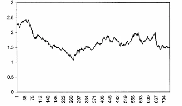
Fig. 2.2: Weekly BP/USD exchange rate series (1980-1993)
Fig. 2.3: Monthly international airline passenger series (Jan. 1949-Dec. 1960)
The first time series is taken from [8] and it represents the weekly exchange rate between British pound and US dollar from 1980 to 1933. The second one is a seasonal time series, considered in [3, 6, 11] and it shows the number of international airline passengers (in thousands) between Jan. 1949 to Dec. 1960 on a monthly basis.
2.4Introduction to Time Series Analysis
In practice a suitable model is fitted to a given time series and the corresponding parameters are estimated using the known data values. The procedure of fitting a time series to a proper model is termed as Time Series Analysis [23]. It comprises methods that attempt to understand the nature of the series and is often useful for future forecasting and simulation.
In time series forecasting, past observations are collected and analyzed to develop a suitable mathematical model which captures the underlying data generating process for the series [7, 8]. The future events are then predicted using the model. This approach is particularly useful when there is not much knowledge about the statistical pattern followed by the successive observations or when there is a lack of a satisfactory explanatory model. Time series forecasting has important applications in various fields. Often valuable strategic decisions and precautionary measures are taken based on the forecast results. Thus making a good forecast, i.e. fitting an adequate model to a time series is vary important. Over the past several decades many efforts have been made by researchers for the development and improvement of suitable time series forecasting models.
2.5Time Series and Stochastic Process
A time series is non-deterministic in nature, i.e. we cannot predict with certainty what will occur in future. Generally a time series
{
x(t),t =0,1,2,. ..}
is assumed to follow certain probability model [21] which describes the joint distribution of the random variable .xt Themathematical expression describing the probability structure of a time series is termed as a stochastic process [23]. Thus the sequence of observations of the series is actually a sample realization of the stochastic process that produced it.
A usual assumption is that the time series variables xt are independent and identically distributed (i.i.d) following the normal distribution. However as mentioned in [21], an interesting point is that time series are in fact not exactly i.i.d; they follow more or less some regular pattern in long term. For example if the temperature today of a particular city is extremely high, then it can be reasonably presumed that tomorrow’s temperature will also likely to be high. This is the reason why time series forecasting using a proper technique, yields result close to the actual value.
2.6 Concept of Stationarity
The concept of stationarity of a stochastic process can be visualized as a form of statistical equilibrium [23]. The statistical properties such as mean and variance of a stationary process do not depend upon time. It is a necessary condition for building a time series model that is useful for future forecasting. Further, the mathematical complexity of the fitted model reduces with this assumption. There are two types of stationary processes which are defined below:
A process
{
x(t),t=0,1,2,...}
is Strongly Stationary or Strictly Stationary if the joint probability distribution function of{
xt−s,xt−s+1,...,xt,...xt+s−1,xt+s}
is independent of t for all s. Thus for a strong stationary process the joint distribution of any possible set of random variables from the process is independent of time [21, 23].However for practical applications, the assumption of strong stationarity is not always needed and so a somewhat weaker form is considered. A stochastic process is said to be Weakly Stationary of order k if the statistical moments of the process up to that order depend only on time differences and not upon the time of occurrences of the data being used to estimate the moments [12, 21, 23]. For example a stochastic process
{
x(t),t =0,1,2,...}
is second order stationary [12, 23] if it has time independent mean and variance and the covariance values) , (xt xt s
Cov − depend only on s.
It is important to note that neither strong nor weak stationarity implies the other. However, a weakly stationary process following normal distribution is also strongly stationary [21]. Some mathematical tests like the one given by Dickey and Fuller [21] are generally used to detect stationarity in a time series data.
As mentioned in [6, 23], the concept of stationarity is a mathematical idea constructed to simplify the theoretical and practical development of stochastic processes. To design a proper model, adequate for future forecasting, the underlying time series is expected to be stationary. Unfortunately it is not always the case. As stated by Hipel and McLeod [23], the greater the time span of historical observations, the greater is the chance that the time series will exhibit non-stationary characteristics. However for relatively short time span, one can reasonably model the series using a stationary stochastic process. Usually time series, showing trend or seasonal patterns are non-stationary in nature. In such cases, differencing and power transformations are often used to remove the trend and to make the series stationary. In the next chapter we shall discuss about the seasonal differencing technique applied to make a seasonal time series stationary.
2.7Model Parsimony
While building a proper time series model we have to consider the principle of parsimony [2, 7, 8, 23]. According to this principle, always the model with smallest possible number of parameters is to be selected so as to provide an adequate representation of the underlying time series data [2]. Out of a number of suitable models, one should consider the simplest one, still maintaining an accurate description of inherent properties of the time series. The idea of model parsimony is similar to the famous Occam’s razor principle [23]. As discussed by Hipel and McLeod [23], one aspect of this principle is that when face with a number of competing and
adequate explanations, pick the most simple one. The Occam’s razor provides considerable inherent informations, when applied to logical analysis.
Moreover, the more complicated the model, the more possibilities will arise for departure from the actual model assumptions. With the increase of model parameters, the risk of overfitting also subsequently increases. An over fitted time series model may describe the training data very well, but it may not be suitable for future forecasting. As potential overfitting affects the ability of a model to forecast well, parsimony is often used as a guiding principle to overcome this issue. Thus in summary it can be said that, while making time series forecasts, genuine attention should be given to select the most parsimonious model among all other possibilities.
Chapter-3
Time Series Forecasting Using Stochastic Models
3.1Introduction
In the previous chapter we have discussed about the fundamentals of time series modeling and forecasting. The selection of a proper model is extremely important as it reflects the underlying structure of the series and this fitted model in turn is used for future forecasting. A time series model is said to be linear or non-linear depending on whether the current value of the series is a linear or non-linear function of past observations.
In general models for time series data can have many forms and represent different stochastic processes. There are two widely used linear time series models in literature, viz. Autoregressive (AR) [6, 12, 23] and Moving Average (MA) [6, 23] models. Combining these two, the Autoregressive Moving Average (ARMA) [6, 12, 21, 23] and Autoregressive Integrated Moving Average (ARIMA) [6, 21, 23] models have been proposed in literature. The Autoregressive Fractionally Integrated Moving Average (ARFIMA) [9, 17] model generalizes ARMA and ARIMA models. For seasonal time series forecasting, a variation of ARIMA, viz. the Seasonal Autoregressive Integrated Moving Average (SARIMA) [3, 6, 23] model is used. ARIMA model and its different variations are based on the famous Box-Jenkins principle [6, 8, 12, 23] and so these are also broadly known as the Box-Jenkins models.
Linear models have drawn much attention due to their relative simplicity in understanding and implementation. However many practical time series show non-linear patterns. For example, as mentioned by R. Parrelli in [28], non-linear models are appropriate for predicting volatility changes in economic and financial time series. Considering these facts, various non-linear models have been suggested in literature. Some of them are the famous Autoregressive Conditional Heteroskedasticity (ARCH) [9, 28] model and its variations like Generalized ARCH (GARCH) [9, 28], Exponential Generalized ARCH (EGARCH) [9] etc., the Threshold Autoregressive (TAR) [8, 10] model, the linear Autoregressive (NAR) [7] model, the Non-linear Moving Average (NMA) [28] model, etc.
In this chapter we shall discuss about the important linear and non-linear stochastic time series models with their different properties. This chapter will provide a background for the upcoming chapters, in which we shall study other models used for time series forecasting.
3.2The Autoregressive Moving Average (ARMA) Models
An ARMA(p, q) model is a combination of AR(p) and MA(q) models and is suitable for univariate time series modeling. In an AR(p) model the future value of a variable is assumed to
be a linear combination of p past observations and a random error together with a constant term. Mathematically the AR(p) model can be expressed as [12, 23]:
t p t p t t p i t i t i t c y c y y y y = + ϕ +ε = +ϕ − +ϕ − + +ϕ − +ε = −
∑
1 1 2 2 ... 1 (3.1) Here yt and εt are respectively the actual value and random error (or random shock) at timeperiod t, )ϕi(i=1,2, ..,.p are model parameters and c is a constant. The integer constant pis known as the order of the model. Sometimes the constant term is omitted for simplicity. Usually For estimating parameters of an AR process using the given time series, the Yule-Walker equations [23] are used.
Just as an AR(p) model regress against past values of the series, an MA(q) model uses past errors as the explanatory variables. The MA(q) model is given by [12, 21, 23]:
t q t q t t q j t j t j t y =μ+ θ ε +ε =μ+θ ε − +θ ε − + +θ ε − +ε = −
∑
1 1 2 2 ... 1 (3.2) Here μ is the mean of the series, θj(j =1,2,.. ,.q) are the model parameters and qis the order of the model. The random shocks are assumed to be a white noise [21, 23] process, i.e. a sequence of independent and identically distributed (i.i.d) random variables with zero mean and a constant variance σ2. Generally, the random shocks are assumed to follow the typical normal distribution. Thus conceptually a moving average model is a linear regression of the current observation of the time series against the random shocks of one or more prior observations. Fitting an MA model to a time series is more complicated than fitting an AR model because in the former one the random error terms are not fore-seeable.Autoregressive (AR) and moving average (MA) models can be effectively combined together to form a general and useful class of time series models, known as the ARMA models. Mathematically an ARMA(p, q) model is represented as [12, 21, 23]:
∑
∑
= − = − + + + = q j j t j p i i t i t t c y y 1 1 ε θ ϕ ε (3.3)Here the model orders p, refer to q p autoregressive and q moving average terms.
Usually ARMA models are manipulated using the lag operator [21, 23] notation. The lag or backshift operator is defined as Lyt = yt−1. Polynomials of lag operator or lag polynomials are used to represent ARMA models as follows [21]:
MA(q) model: yt =θ(L)εt. ARMA(p, q) model: ϕ(L)yt =θ(L)εt. Here
∑
∑
= = + = − = q j j j i p i iL and L L L 1 1 . 1 ) ( 1 ) ( ϕ θ θ ϕIt is shown in [23] that an important property of AR(p) process is invertibility, i.e. an AR(p) process can always be written in terms of an MA(∞) process. Whereas for an MA(q) process to be invertible, all the roots of the equation θ(L)=0 must lie outside the unit circle. This condition is known as the Invertibility Condition for an MA process.
3.3Stationarity Analysis
When an AR(p) process is represented as εt =ϕ(L)yt, then ϕ(L)=0 is known as the
characteristic equation for the process. It is proved by Box and Jenkins [6] that a necessary and sufficient condition for the AR(p) process to be stationary is that all the roots of the characteristic equation must fall outside the unit circle. Hipel and McLeod [23] mentioned another simple algorithm (by Schur and Pagano) for determining stationarity of an AR process. For example as shown in [12] the AR(1) model yt =c+ϕ1yt−1 +εt is stationary when ϕ1 <1, with a constant mean
1 1 ϕ
μ
−
= c and constant variance .
1 2 1 2 0 ϕ σ γ − =
An MA(q) process is always stationary, irrespective of the values the MA parameters [23]. The conditions regarding stationarity and invertibility of AR and MA processes also hold for an ARMA process. An ARMA(p, q) process is stationary if all the roots of the characteristic equation ϕ(L)=0 lie outside the unit circle. Similarly, if all the roots of the lag equation
0 ) (L =
θ lie outside the unit circle, then the ARMA(p, q) process is invertible and can be expressed as a pure AR process.
3.4Autocorrelation and Partial Autocorrelation Functions (ACF and PACF)
To determine a proper model for a given time series data, it is necessary to carry out the ACF and PACF analysis. These statistical measures reflect how the observations in a time series are related to each other. For modeling and forecasting purpose it is often useful to plot the ACF and PACF against consecutive time lags. These plots help in determining the order of AR and MA terms. Below we give their mathematical definitions:
For a time series
{
x(t),t =0,1,2,...}
the Autocovariance [21, 23] at lag k is defined as: )] )( [( ) , ( μ μ γk =Cov xt xt+k = E xt − xt+k − (3.4)The Autocorrelation Coeffient [21, 23] at lag k is defined as: 0 γ γ ρ k k = (3.5)
Here μis the mean of the time series, i.e. μ =E[xt]. The autocovariance at lag zero i.e. γ0 is the variance of the time series. From the definition it is clear that the autocorrelation coefficient
k
ρ is dimensionless and so is independent of the scale of measurement. Also, clearly .
1
1≤ ≤
− ρk Statisticians Box and Jenkins [6] termed γk as the theoretical Autocovariance
Function (ACVF) and ρk as the theoretical Autocorrelation Function (ACF).
Another measure, known as the Partial Autucorrelation Function (PACF) is used to measure the correlation between an observation k period ago and the current observation, after controlling for observations at intermediate lags (i.e. at lags <k) [12]. At lag 1, PACF(1) is same as ACF(1). The detailed formulae for calculating PACF are given in [6, 23].
Normally, the stochastic process governing a time series is unknown and so it is not possible to determine the actual or theoretical ACF and PACF values. Rather these values are to be estimated from the training data, i.e. the known time series at hand. The estimated ACF and PACF values from the training data are respectively termed as sample ACF and PACF [6, 23]. As given in [23], the most appropriate sample estimate for the ACVF at lag k is
∑
− = + − − = n k t k t t k x x n c 1 ) )( ( 1 μ μ (3.6) Then the estimate for the sample ACF at lag k is given by0 c c
r k
k = (3.7)
Here
{
x(t),t =0,1,2,...}
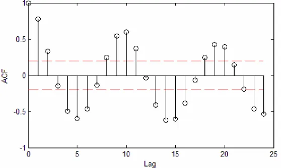
is the training series of size n with meanμ.As explained by Box and Jenkins [6], the sample ACF plot is useful in determining the type of model to fit to a time series of length N. Since ACF is symmetrical about lag zero, it is only required to plot the sample ACF for positive lags, from lag one onwards to a maximum lag of about N/4. The sample PACF plot helps in identifying the maximum order of an AR process. The methods for calculating ACF and PACF for ARMA models are described in [23]. We shall demonstrate the use of these plots for our practical datasets in Chapter 7.
3.5Autoregressive Integrated Moving Average (ARIMA) Models
The ARMA models, described above can only be used for stationary time series data. However in practice many time series such as those related to socio-economic [23] and
business show non-stationary behavior. Time series, which contain trend and seasonal patterns, are also non-stationary in nature [3, 11]. Thus from application view point ARMA models are inadequate to properly describe non-stationary time series, which are frequently encountered in practice. For this reason the ARIMA model [6, 23, 27] is proposed, which is a generalization of an ARMA model to include the case of non-stationarity as well.
In ARIMA models a non-stationary time series is made stationary by applying finite differencing of the data points. The mathematical formulation of the ARIMA(p,d,q) model using lag polynomials is given below [23, 27]:
(
)
t j q j j t d i p i i t t d L y L L e i L y L L ε θ ϕ ε θ ϕ ⎟⎟ ⎠ ⎞ ⎜⎜ ⎝ ⎛ + = − ⎟⎟ ⎠ ⎞ ⎜⎜ ⎝ ⎛ − = −∑
∑
= =1 1 1 1 1 . . , ) ( ) 1 )( ( (3.8)• Here, p, d and q are integers greater than or equal to zero and refer to the order of the autoregressive, integrated, and moving average parts of the model respectively.
• The integer d controls the level of differencing. Generally d=1 is enough in most cases. When d=0, then it reduces to an ARMA(p,q) model.
• An ARIMA(p,0,0) is nothing but the AR(p) model and ARIMA(0,0,q) is the MA(q) model.
• ARIMA(0,1,0), i.e. yt = yt−1 +εt is a special one and known as the Random Walk model
[8, 12, 21]. It is widely used for non-stationary data, like economic and stock price series.
A useful generalization of ARIMA models is the Autoregressive Fractionally Integrated Moving Average (ARFIMA) model, which allows non-integer values of the differencing parameter d. ARFIMA has useful application in modeling time series with long memory [17]. In this model the expansion of the term
(
)
dL
−
1 is to be done by using the general binomial theorem. Various contributions have been made by researchers towards the estimation of the general ARFIMA parameters.
3.6Seasonal Autoregressive Integrated Moving Average (SARIMA) Models
The ARIMA model (3.8) is for non-seasonal non-stationary data. Box and Jenkins [6] have generalized this model to deal with seasonality. Their proposed model is known as the Seasonal ARIMA (SARIMA) model. In this model seasonal differencing of appropriate order is used to remove non-stationarity from the series. A first order seasonal difference is the difference between an observation and the corresponding observation from the previous year and is calculated as zt = yt −yt−s. For monthly time series s=12 and for quarterly time series
. 4
=
The mathematical formulation of a s Q D P q d p, , ) ( , , ) (
SARIMA × model in terms of lag
polynomials is given below [13]:
. ) ( ) ( ) ( ) ( . . , ) ( ) ( ) 1 ( ) 1 )( ( ) ( t q s Q t p s P t q s Q t D s d p s P L L z L L e i L L y L L L L ε θ ϕ ε θ ϕ Θ = Φ Θ = − − Φ (3.9)
Here zt is the seasonally differenced series.
3.7Some Nonlinear Time Series Models
So far we have discussed about linear time series models. As mentioned earlier, nonlinear models should also be considered for better time series analysis and forecasting. Campbell, Lo and McKinley (1997) made important contributions towards this direction. According to them almost all linear time series can be divided into two branches: one includes models non-linear in mean and other includes models non-non-linear in variance (heteroskedastic). As an illustrative example, here we present two nonlinear time series models from [28]:
• Nonlinear Moving Average (NMA) Model: .2 1 −
+
= t t
t
y ε αε This model is non-linear in mean but not in variance.
• Eagle’s (1982) ARCH Model: 2.
t t
t
y =ε +α ε This model is heteroskedastic, i.e. non-linear in variance, but non-linear in mean. This model has several other variations, like GARCH, EGARCH etc.
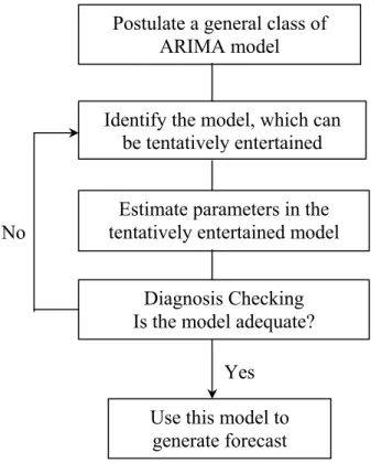
3.8Box-Jenkins Methodology
After describing various time series models, the next issue to our concern is how to select an appropriate model that can produce accurate forecast based on a description of historical pattern in the data and how to determine the optimal model orders. Statisticians George Box and Gwilym Jenkins [6] developed a practical approach to build ARIMA model, which best fit to a given time series and also satisfy the parsimony principle. Their concept has fundamental importance on the area of time series analysis and forecasting [8, 27].
The Box-Jenkins methodology does not assume any particular pattern in the historical data of the series to be forecasted. Rather, it uses a three step iterative approach of model identification, parameter estimation and diagnostic checking to determine the best parsimonious model from a general class of ARIMA models [6, 8, 12, 27]. This three-step process is repeated several times until a satisfactory model is finally selected. Then this model can be used for forecasting future values of the time series.
Fig. 3.1: The Box-Jenkins methodology for optimal model selection
A crucial step in an appropriate model selection is the determination of optimal model parameters. One criterion is that the sample ACF and PACF, calculated from the training data should match with the corresponding theoretical or actual values [11, 13, 23]. Other widely used measures for model identification are Akaike Information Criterion (AIC) [11, 13] and Bayesian Information Criterion (BIC) [11, 13] which are defined below [11]:
) ln( ) ˆ ln( ) ( 2 ) ˆ ln( ) ( 2 2 n p p n n p BIC p n n p AIC e e + + = + = σ σ
Here n is the number of effective observations, used to fit the model, p is the number of parameters in the model and ˆ2
e
σ is the sum of sample squared residuals. The optimal model order is chosen by the number of model parameters, which minimizes either AIC or BIC. Other similar criteria have also been proposed in literature for optimal model identification.
Postulate a general class of ARIMA model
Identify the model, which can be tentatively entertained
Estimate parameters in the tentatively entertained model
Diagnosis Checking Is the model adequate?
Use this model to generate forecast
Yes No
Chapter-4
Time Series Forecasting Using Artificial Neural Networks
4.1Artificial Neural Networks (ANNs)
In the previous Chapter we have discussed the important stochastic methods for time series modeling and forecasting. Artificial neural networks (ANNs) approach has been suggested as an alternative technique to time series forecasting and it gained immense popularity in last few years. The basic objective of ANNs was to construct a model for mimicking the intelligence of human brain into machine [13, 20]. Similar to the work of a human brain, ANNs try to recognize regularities and patterns in the input data, learn from experience and then provide generalized results based on their known previous knowledge. Although the development of ANNs was mainly biologically motivated, but afterwards they have been applied in many different areas, especially for forecasting and classification purposes [13, 20]. Below we shall mention the salient features of ANNs, which make them quite favorite for time series analysis and forecasting.
First, ANNs are data-driven and self-adaptive in nature [5, 20]. There is no need to specify a particular model form or to make any a priori assumption about the statistical distribution of the data; the desired model is adaptively formed based on the features presented from the data. This approach is quite useful for many practical situations, where no theoretical guidance is available for an appropriate data generation process.
Second, ANNs are inherently non-linear, which makes them more practical and accurate in modeling complex data patterns, as opposed to various traditional linear approaches, such as ARIMA methods [5, 8, 20]. There are many instances, which suggest that ANNs made quite better analysis and forecasting than various linear models.
Finally, as suggested by Hornik and Stinchcombe [22], ANNs are universal functional approximators. They have shown that a network can approximate any continuous function to any desired accuracy [5, 22]. ANNs use parallel processing of the information from the data to approximate a large class of functions with a high degree of accuracy. Further, they can deal with situation, where the input data are erroneous, incomplete or fuzzy [20].
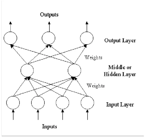
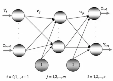
4.2The ANN Architecture
The most widely used ANNs in forecasting problems are multi-layer perceptrons (MLPs), which use a single hidden layer feed forward network (FNN) [5,8]. The model is characterized by a network of three layers, viz. input, hidden and output layer, connected by acyclic links. There may be more than one hidden layer. The nodes in various layers are also known as
processing elements. The three-layer feed forward architecture of ANN models can be diagrammatically depicted as below:
Fig. 4.1: The three-layer feed forward ANN architecture
The output of the model is computed using the following mathematical expression [7]: t y g y q j t p i i t ij j j t ⎟⎟+ ∀ ⎠ ⎞ ⎜⎜ ⎝ ⎛ + + =
∑
∑
= = − , 1 1 0 0 α β β ε α (4.1)Here )yt−i(i =1,2,..,.p are the p inputs and yt is the output. The integers p, q are the number of input and hidden nodes respectively. αj(j=0,1,2, ..,.q) and βij(i=0,1,2, ..,.p;j =0,1,2, ..,.q) are the connection weights and εt is the random shock; α0 and β0j are the bias terms. Usually, the logistic sigmoid function x
e x g − + = 1 1 )
( is applied as the nonlinear activation function. Other activation functions, such as linear, hyperbolic tangent, Gaussian, etc. can also be used [20].
The feed forward ANN model (4.1) in fact performs a non-linear functional mapping from the past observations of the time series to the future value, i.e. yt = f(yt−1,yt−2,...yt−p,w)+εt,
where wis a vector of all parameters and f is a function determined by the network structure and connection weights [5, 8].
To estimate the connection weights, non-linear least square procedures are used, which are based on the minimization of the error function [13]:
∑
∑
= − = Ψ t t t t t y y e F( ) 2 ( ˆ )2 (4.2) Here Ψis the space of all connection weights.The optimization techniques used for minimizing the error function (4.2) are referred as Learning Rules. The best-known learning rule in literature is the Backpropagation or Generalized Delta Rule [13, 20].
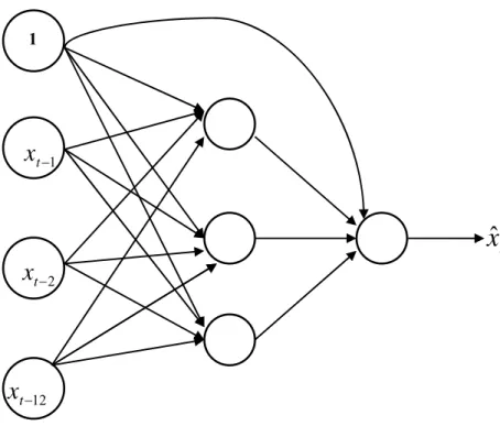
4.3Time Lagged Neural Networks (TLNN)
In the FNN formulation, described above, the input nodes are the successive observations of the time series, i.e. the target xt is a function of the valuesxt−i,(i=1,2, ..,.p) where p is the number of input nodes. Another variation of FNN, viz. the TLNN architecture [11, 13] is also widely used. In TLNN, the input nodes are the time series values at some particular lags. For example, a typical TLNN for a time series, with seasonal period s =12 can contain the input nodes as the lagged values at time t−1, t−2 and t−12.The value at time t is to be forecasted using the values at lags 1, 2 and 12.
Fig. 4.2: A typical TLNN architecture for monthly data
1 1 − t
x
12 − tx
2 − tx
tx
ˆ
In addition, there is a constant input term, which may be conveniently taken as 1 and this is connected to every neuron in the hidden and output layer. The introduction of this constant input unit avoids the necessity of separately introducing a bias term.
For a TLNN with one hidden level, the general prediction equation for computing a forecast may be written as [11]: ⎭ ⎬ ⎫ ⎩ ⎨ ⎧ ⎟ ⎠ ⎞ ⎜ ⎝ ⎛ + + + =
∑
∑
− h i j t ih ch h h c t w w w w x i xˆ φ0 0 0φ (4.3) Here, the selected past observationsk j t j t j t x x
x−1, − 2, ..,. − are the input terms,
{ }
wch are theweights for the connections between the constant input and hidden neurons and wc0 is the weight of the direct connection between the constant input and the output. Also
{ }
wih and{ }
wh0 denote the weights for other connections between the input and hidden neurons and between the hidden and output neurons respectively. φh and φ0 are the hidden and output layer activation functions respectively.Faraway and Chatfield [11] used the notation NN(j1,j2,..,.jk;h) to denote the TLNN with inputs at lags j1,j2, ..,.jk and h hidden neurons. We shall also adopt this notation in our
upcoming experiments. Thus Fig. 4.2 represents an NN (1, 2, 12; 3) model.
4.4Seasonal Artificial Neural Networks (SANN)
The SANN structure is proposed by C. Hamzacebi [3] to improve the forecasting performance of ANNs for seasonal time series data. The proposed SANN model does not require any preprocessing of raw data. Also SANN can learn the seasonal pattern in the series, without removing them, contrary to some other traditional approaches, such as SARIMA, discussed in Chapter 3. The author has empirically verified the good forecasting ability of SANN on four practical time data sets. We have also used this model in our current work on two new seasonal time series and obtained quite satisfactory results. Here we present a brief overview of SANN model as proposed in [3].
In this model, the seasonal parameter s is used to determine the number of input and output neurons. This consideration makes the model surprisingly simple for understanding and implementation. The ith and (i+1)th seasonal period observationsare respectively used as the values of input and output neurons in this network structure. Each seasonal period is composed of a number of observations.
Fig. 4.3: SANN architecture for seasonal time series
Mathematical expression for the output of the model is [3]:
. ,. .. , 3 , 2 , 1 ; 1 1 0 s l t Y v f w Y m j s i i t ij j jl l l t ⎟ ∀ = ⎠ ⎞ ⎜ ⎝ ⎛ + + =
∑
∑
= − = − + α θ (4.4)Here )Yt+l(l =1,2,3,..,.s are the predictions for the future s periods and Yt−i(i=0,1,2,..,.s−1)are the observations of the previous s periods; vij(i=0,1,2,..,.s−1;j =1,2,3,..,.m)are weights of connections from input nodes to hidden nodes and wjl (j =1,2,3,..,.m;l =1,2,3,..,.s)are weights of connections from hidden nodes to output nodes. Also αl(l=1,2,3, ..,.s)and
) ,. .. , 3 , 2 , 1 (j m j =
θ are weights of bias connection and f is the activation function.
Thus while forecasting with SANN, the number of input and output neurons should be taken as 12 for monthly and 4 for quarterly time series. The appropriate number of hidden nodes can be determined by performing suitable experiments on the training data.
4.5Selection of A Proper Network Architecture
So far we have discussed about three important network architectures, viz. the FNN, TLNN and SANN, which are extensively used in forecasting problems. Some other types of neural models are also proposed in literature, such as the Probabilistic Neural Network (PNN) [20] for classification problem and Generalized Regression Neural Network (GRNN) [20] for regression problem. After specifying a particular network structure, the next most important issue is the
determination of the optimal network parameters. The number of network parameters is equal to the total number of connections between the neurons and the bias terms [3, 11].
A desired network model should produce reasonably small error not only on within sample (training) data but also on out of sample (test) data [20]. Due to this reason immense care is required while choosing the number of input and hidden neurons. However, it is a difficult task as there is no theoretical guidance available for the selection of these parameters and often experiments, such as cross-validation are conducted for this purpose [3, 8].
Another major problem is that an inadequate or large number of network parameters may lead to the overtraining of data [2, 11]. Overtraining produces spuriously good within-sample fit, which does not generate better forecasts. To penalize the addition of extra parameters some model comparison criteria, such as AIC and BIC can be used [11, 13]. Network Pruning [13] and MacKay’s Bayesian Regularization Algorithm [11, 20] are also quite popular in this regard.
In summary we can say that NNs are amazingly simple though powerful techniques for time series forecasting. The selection of appropriate network parameters is crucial, while using NN for forecasting purpose. Also a suitable transformation or rescaling of the training data is often necessary to obtain best results.
Chapter-5
Time Series Forecasting Using Support Vector Machines
5.1Concept of Support Vector Machines
Till now, we have studied about various stochastic and neural network methods for time series modeling and forecasting. Despite of their own strengths and weaknesses, these methods are quite successful in forecasting applications. Recently, a new statistical learning theory, viz. the Support Vector Machine (SVM) has been receiving increasing attention for classification and forecasting [18, 24, 30, 31]. SVM was developed by Vapnik and his co-workers at the AT & T Bell laboratories in 1995 [24, 29, 33]. Initially SVMs were designed to solve pattern classification problems, such as optimal character recognition, face identification and text classification, etc. But soon they found wide applications in other domains, such as function approximation, regression estimation and time series prediction problems [24, 31, 34].
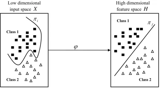
Vapnik’s SVM technique is based on the Structural Risk Minimization (SRM) principle [24, 29, 30]. The objective of SVM is to find a decision rule with good generalization ability through selecting some particular subset of training data, called support vectors [29, 31, 33]. In this method, an optimal separating hyperplane is constructed, after nonlinearly mapping the input space into a higher dimensional feature space. Thus, the quality and complexity of SVM solution does not depend directly on the input space [18, 19].
Another important characteristic of SVM is that here the training process is equivalent to solving a linearly constrained quadratic programming problem. So, contrary to other networks’ training, the SVM solution is always unique and globally optimal. However a major disadvantage of SVM is that when the training size is large, it requires an enormous amount of computation which increases the time complexity of the solution [24].
Now we are going to present a brief mathematical discussion about SVM concept.
5.2Introduction to Statistical Learning Theory
Vapnik’s statistical learning theory is developed in order to derive a learning technique which will provide good generalization. According to Vapnik [33] there are three main problems in machine learning, viz. Classification, Regression and Density Estimation. In all these cases the main goal is to learn a function (or hypothesis) from the training data using a learning machine and then infer general results based on this knowledge.
In case of supervised learning the training data is composed of pairs of input and output variables. The input vectors n
X ⊆ℜ
∈
x and the output points y∈D⊆ℜ. The two sets X and D are respectively termed as the input space and output space [29, 33]. D=
{
−1,1} { }
or 0,1 for binary classification problem and D=ℜ for regression problem.In case of unsupervised learning the training data is composed of only the input vectors. Here the main goal is to infer the inherent structure of the data through density estimation and clustering technique.
The training data is supposed to be generated from an i.i.d process following an unknown distribution )P(x,y defined on the set X ×D. An input vector is drawn from X with the marginal probability P(x) and the corresponding output point is observed in D with the conditional probabilityP(yx).
Fig. 5.1: Probabilistic mapping of input and output points
After these descriptions, the learning problem can be visualized as searching for the appropriate estimator function f :X →D which will represent the process of output generations from the input vectors [29, 33]. This function then can be used for generalization, i.e. to produce an output value in response to an unseen input vector.
5.3Empirical Risk Minimization (ERM)
We have seen that the main aim of statistical learning theory is to search for the most appropriate estimator function f :X →D which maps the points of the input space X to the output space D. Following Vapnik and Chervonenkis (1971) first a Risk Functional is defined on X×D to measure the average error occurred among the actual and predicted (or classified) outputs due to using an estimator function .f Then the most suitable estimator function is chosen to be that function which minimizes this risk [29, 30, 33].
Let us consider the set of functions F =
{
f(x,w)}
that map the points from the input spacen
X ⊆ℜ into the output space D⊆ℜ where w denotes the parameters defining .f Also )
(x
P P(yx)
suppose that y be the actual output point corresponding to the input vector x. Now if )) , ( , (y f x w
L measures the error between the actual valueyand the predicted value f(x,w)for using the prediction function f then the Expected Risk is defined as [29, 33]:
∫
= ( , ( , )) ( , )
)
(f L y f dP y
R x w x (5.1) Here )P(x,y is the probability distribution followed by the training data. L(y,f(x,w)) is known as the Loss Function and it can be defined in a number of ways [24, 29, 30].
The most suitable prediction function is the one which minimizes the expected risk R(f) and is denoted by .f0 This is known as the Target Function. The main task of learning problem is now to find out this target function, which is the ideal estimator. Unfortunately this is not possible because the probability distribution P(x,y) of the given data is unknown and so the expected risk (5.1) cannot be computed. This critical problem motivates Vapnik to suggest the Empirical Risk Minimization (ERM) principle [33].
The concept of ERM is to estimate the expected risk R(f)by using the training set. This approximation of R(f) is called the empirical risk. For a given training set
{
xi,yi}
, where) ,. .. , 3 , 2 , 1 ( ,y D i N X n i i∈ ⊆ℜ ∈ ⊆ℜ ∀ =
x the empirical risk is defined as [29, 33]:
∑
= = N i i i emp L y f N f R 1 )) , ( , ( 1 ) ( x w (5.2)The empirical risk Remp(f) has its own minimizer inF , which can be taken asfˆ. The goal of ERM principle is to approximate the target function f0 by fˆ. This is possible due to the result that R(f) infact converges to Remp(f) when the training size N is infinitely large [33].
5.4Vapnik-Chervonenkis (VC) Dimension
The VC dimension h of a class of functions F is defined as the maximum number of points that can be exactly classified (i.e. shattered) by F [29, 33]. So mathematically [1, 33]:
{
}
{
, ,suchthat 1,1 , suchthat 1}
.max n X i i i b ) f(x N), i ( X x F f b X X h= ⊆ℜ ∀ ∈ − ∃ ∈ ∀ ∈ ≤ ≤ =
The VC dimension is infact a measure of the intrinsic capacity of a class of functionsF. It is proved by Burges in 1998 [1] that the VC dimension of the set of oriented hyperplanes in ℜn
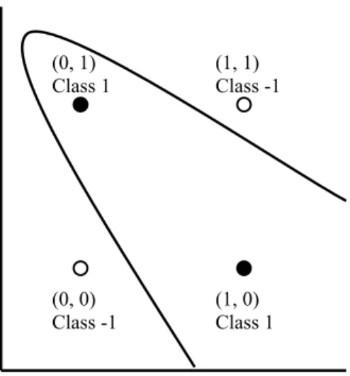
is )(n+1 . Thus three points labeled in eight different ways can always be classified by a linear oriented decision boundary in ℜ2 but four points cannot. Thus VC dimension of the set of oriented straight lines in ℜ2 is three. For example the XOR problem [29] cannot be realized using a linear decision boundary. However a quadratic decision boundary can correctly classify the points in this problem. This is shown in the figures below:
(a)The linearly non-separable (b)A quadratic decision boundary
XOR problem classifying the XOR problem Fig. 5.2: The two-dimensional XOR problem
5.5Structural Risk Minimization (SRM)
The crucial shortcoming of ERM principle is that in practice we always have a finite set of observations and so it cannot be guaranteed that the estimator function minimizing the empirical risk over F will also minimize the expected risk. To deal with this issue the SRM principle was developed by Vapnik and Chervonenkis in 1982 [33]. The key result motivating this principle is that the difference between the empirical and expected risk can be bounded in terms of the VC dimension of the class F of estimator functions. Below we present the corresponding mathematical theorem for
{ }
0,1 binary classification problem [29]:Theorem: Let F be a class of estimator functions of VC dimension h. Then for any
sample
{
xi,yi}
, where X ,yi D ( i 1,2,3, ..,.N)n
i∈ ⊆ℜ ∈ ⊆ℜ ∀ =
x drawn from any distribution
) , ( y
P x the following bound holds true with probability1−η (0≤η ≤1):
N h N h f R f R emp ⎟ ⎠ ⎞ ⎜ ⎝ ⎛ − ⎟⎟ ⎠ ⎞ ⎜⎜ ⎝ ⎛ + ⎟ ⎠ ⎞ ⎜ ⎝ ⎛ + ≤ 4 ln 1 2 ln ) ( ) ( η (5.3) The second term on the right is said to be the VC Confidence and 1−η is called the Confidence Level.
Equation (4.3) is the main inspiration behind the SRM principle. It suggests that to achieve a good generalization one has to minimize the combination of the empirical risk and the complexity of the hypothesis space. In other words one should try to select that hypothesis space which realizes the best trade-off between small empirical error and small model complexity. This concept is similar to the Bias-Variance Dilemma of machine learning [29].
(0, 0) Class -1 (1, 0) Class 1 (1, 1) Class -1 (0, 1) Class 1 (0, 0) Class -1 (1, 0) Class 1 (1, 1) Class -1 (0, 1) Class 1
5.6Support Vector Machines (SVMs)
The main idea of SVM when applied to binary classification problems is to find a canonical hyperplane which maximally separates the two given classes of training samples [18, 24, 29, 31, 33]. Let us consider two sets of linearly separable training data points in ℜn
which are to be classified into one of the two classes C1and C2 using linear hyperplanes, (i.e. straight lines). From an infinite number of separating hyperplanes the one with maximum margin is to be selected for best classification and generalization [29, 33]. Below we present a diagrammatic view of this concept:
(a) Infinite number of linearly (b) The maximum margin hyperplane
separating hyperplanes
Fig. 5.3: Support vectors for linearly separable data points
In Fig.4.3(a) it can be seen that there are an infinite number of hyperplanes, separating the training data points. As shown in Fig.4.3(b), d+ and d− denote the perpendicular distances from the separating hyperplane to the closest data points of C1and C2 respectively. Then either of the distances d+or d− is termed as the margin and the total margin is
.
− + +
=d d
M For accurate classification as well as best generalization, the hyperplane which maximizes the total margin is considered as the optimal one and is known as the Maximum Margin Hyperplane [29, 33]. Offcourse for this optimal hyperplane d+ =d−[29]. The data points from either of the two classes which are closest to the maximum margin hyperplane are known as Support Vectors [29, 33]. In Fig.4.3(b) π denotes the optimal hyperplane and circulated data points of both the classes represent the support vectors.
Class C2 Class C1
π
+ d − d Class C2 Class C1Let us consider that the training set is composed of the input-output pairs
{
}
N i i i,y =1 x , where{
1,1}
. , ∈ − ℜ ∈ i n i yx The goal is to classify the data points into two classes by finding a maximum margin canonical hyperplane. The hypothesis space is the set of functions
) sgn( ) , , ( b b
f x w = wTx+ where w is the weight vector, x∈ℜn and b is the bias term. The set of separating hyperplanes is given by
{
x∈ℜn :wTx+b=0,wherew∈ℜn,b∈ℜ}
. Using SVM the problem of finding the maximum margin hyperplane reduces to solving a non-linear convex quadratic programming problem (QPP) [29, 32, 33].SVM for Linearly Separable Data
For linearly separable data the corresponding quadratic optimization problem is [18, 29, 33]:
⎪⎭ ⎪ ⎬ ⎫ = ∀ ≥ + = = N i b y J i T i T , . . . , 2 , 1 ; 1 ) ( Subject to 2 1 2 1 ) ( Minimize 2 x w w w w w (5.4)
To solve the QPP (5.4) it is conveniently transformed to the dual space. Then Lagrange multipliers and Kühn-Tucker complimentary conditions are used to find the optimal solution. Let us consider that the solution to the QPP yields