Performance of state space and ARIMA models for consumer retail sales forecasting

Performance of state space and ARIMA models for consumer retail

sales forecasting

Patrícia Ramos

, Nicolau Santos

, Rui Rebelo

School of Accounting and Administration of Porto, Polytechnic Institute of Porto, 4465-004 S. Mamede de Infesta, Portugal b_{INESC Technology and Science, Manufacturing Systems Engineering Unit, 4200-465 Porto, Portugal}

a r t i c l e i n f o

Received 26 March 2014 Received in revised form 10 December 2014 Accepted 29 December 2014 Available online 22 January 2015 Keywords:

Aggregate retail sales Forecast accuracy State space models ARIMA models

a b s t r a c t

Forecasting future sales is one of the most important issues that is beyond all strategic and planning decisions in effective operations of retail businesses. For profitable retail businesses, accurate demand forecasting is crucial in organizing and planning production, purchasing, transportation and labor force. Retail sales series belong to a special type of time series that typically contain trend and seasonal pat-terns, presenting challenges in developing effective forecasting models. This work compares the fore-casting performance of state space models and ARIMA models. The forefore-casting performance is demon-strated through a case study of retail sales offive different categories of women footwear: Boots, Booties, Flats, Sandals and Shoes. On both methodologies the model with the minimum value of Akaike's In-formation Criteria for the in-sample period was selected from all admissible models for further eva-luation in the out-of-sample. Both one-step and multiple-step forecasts were produced. The results show that when an automatic algorithm the overall out-of-sample forecasting performance of state space and ARIMA models evaluated via RMSE, MAE and MAPE is quite similar on both one-step and multi-step forecasts. We also conclude that state space and ARIMA produce coverage probabilities that are close to the nominal rates for both one-step and multi-step forecasts.

&2015 Elsevier Ltd. All rights reserved.

1. Introduction

Sales forecasting is one of the most important issues that is beyond all strategic and planning decisions in any retail business. The importance of accurate sales forecasts to efficient inventory management at both disaggregate and aggregate levels has long been recognized[1]. Poor forecasts usually lead to either too much or too little inventory directly affecting the profitability and the competitive position of the company. At the organizational level, sales forecasting is very important to any retail business as its outcome is used by many functions in the organization:finance and accounting departments are able to project costs, pro_fit levels and capital needs; sales department is able to get a good knowl-edge of the sales volume of each product; purchasing department is able to plan short- and long-term purchases; marketing de-partment is able to plan its actions and assess the impact of dif-ferent marketing strategies on sales volume; andfinally logistics department is able to define specific logistic needs[2]. Accurate forecasts of sales have the potential to increase the profitability of

retailers by improving the chain operations efficiency and mini-mizing wastes. Moreover, accurate forecasts of retail sales may improve portfolio investors’ability to predict movements in the stock prices of retailing chains [3]. Aggregate retail sales time series are usually preferred because they contain both trend and seasonal patterns, providing a good testing ground for comparing forecasting methods, and because companies can benefit from more accurate forecasts.

Retail sales time series often exhibit strong trend and seasonal variations presenting challenges in developing effective forecast-ing models. How to effectively model retail sales series and how to improve the quality of forecasts are still outstanding questions. Exponential smoothing and Autoregressive Integrated Moving Average (ARIMA) models are the two most widely used ap-proaches to time series forecasting, and provide complementary approaches to the problem. While exponential smoothing meth-ods are based on a description of trend and seasonality in the data, ARIMA models aim to describe the autocorrelations in the data. The ARIMA framework to forecasting originally developed by Box et al.[4]involves an iterative three-stage process of model selec-tion, parameter estimation and model checking. A statistical fra-mework to exponential smoothing methods was recently devel-oped based on state space models called ETS models[5].

Despite the investigator's efforts, the several existing studies Contents lists available atScienceDirect

journal homepage:www.elsevier.com/locate/rcim

Robotics and Computer-Integrated Manufacturing

http://dx.doi.org/10.1016/j.rcim.2014.12.015 0736-5845/&2015 Elsevier Ltd. All rights reserved.

n_{Corresponding author at: INESC Technology and Science, Manufacturing} Sys-tems Engineering Unit, 4200-465 Porto, Portugal.

E-mail addresses:[email protected](P. Ramos),

have not led to a consensus about the relative forecasting perfor-mances of these two modeling frameworks when they are applied to retail sales data. Alon [6] concluded that the Winters ex-ponential smoothing method' forecasts of aggregate retail sales were more accurate than the simple and Holt exponential smoothing methods' forecasts. Additionally, Alon et al. [3] com-pared out-of-sample forecasts of aggregated retail sales made using artificial neural networks (ANNs), Winters exponential smoothing, ARIMA and multiple regression via MAPE (mean ab-solute percentage error). Their results indicate that Winters ex-ponential smoothing and ARIMA perform well when macro-economic conditions are relatively stable. When macro-economic condi-tions are volatile (supply push inflation, recessions, high interest rates and high unemployment) ANNs outperform the linear methods and multi-step forecasts may be preferred. Chu and Zhang[7]also conducted a comparative study of linear and non-linear models for aggregate retail sales forecasting. The non-linear models studied were the ARIMA model, regression with dummy variables and regression with trigonometric variables. The non-linear models studied were the ANNs for which the effect of sea-sonal adjustment and use of dummy or trigonometric variables was investigated. Using multiple cross-validation samples eval-uated via the RMSE (root mean squared error), the MAE (mean absolute error) and MAPE, the authors concluded that no single forecasting model is the best for all situations under all circum-stances. Their empirical results show that (1) prior seasonal ad-justment of the data can significantly improve forecasting perfor-mance of the neural network model; (2) seasonal dummy vari-ables can be useful in developing effective regression models (linear and nonlinear) but the performance of these dummy re-gression models may not always be robust; (3) trigonometric models are not useful in aggregate retail sales forecasting. Another interesting example is by Frank et al.[8]forecast women's apparel sales using single seasonal exponential smoothing (SSES), the Winters' three parameter model and ANNs. The performance of the models was tested by comparing the goodness-of-_fit statistics

R2 _{and by comparing actual sales with the forecasted sales of}

different types of garments. Their results indicated that the three parameter Winters' model outperformed SSES in terms ofR2_and

forecasting sales. ANN model performed best in terms of R2

(among three models) but correlations between actual and fore-casted sales were not satisfactory. Zhang and Qi[9]and Kuvulmaz et al.[10]further investigated the use of ANNs in forecasting time series with strong trend and seasonality and conclude that the overall out-of-sample forecasting performance of ANNs, evaluated via RMSE, MAE and MAPE, is not better than ARIMA models in predicting retail sales without appropriate data preprocessing namely detrending and deseasonalization. Motivated by the par-ticular advantages of ARIMA models and ANNs, Aburto and Weber

[11]developed a hybrid intelligent system combining ARIMA type approaches and MLP-type neural networks for demand forecasting that showed improvements in forecasting accuracy. Encouraged by their results they proposed a replenishment system for a Chilean supermarket which led simultaneously to fewer sales failures and lower inventory levels. Motivated by the recent success of evolu-tionary computation Au et al.[12]studied the use of evolutionary neural networks (ENNs) for sales forecasting in fashion retailing. Their experiments show that when guided with the BIC (Bayesian Information Criterion) and the pre-search approach, the ENN can converge much faster and be more accurate in forecasting than the fully connected neural network. The authors also conclude that the performance of these algorithms is better than the performance of the ARIMA model only for products with features of low demand uncertainty and weak seasonal trends. Further, it is emphasized that the ENN approach for forecasting is a highly automatic one while the ARIMA modeling involves more human knowledge.

Wong and Guo[13]propose a hybrid intelligent model using ex-treme learning machine (ELM) and a harmony search algorithm to forecast medium-term sales in fashion retail supply chains. The authors show that the proposed model exhibits superior out-of-sample forecasting performance over the ARIMA, ENN and ELM models when evaluated via RMSE, MAPE and MASE (mean abso-lute scaled error). However, they also observe that the perfor-mance of the proposed model deteriorated when the time series was irregular and random pointing that it may not work well with high irregularity and nonlinearity. Finally, Pan et al. [14] in-vestigate the feasibility and potential of applying empirical mode decomposition (EMD) in forecasting aggregate retail sales. The hybrid forecasting method of integrating EMD and neural network models (EMD-NN) was compared with the direct NN model and the ARIMA model for aggregate retail sales forecasting. Data from two sampling periods with different macroeconomic conditions were studied. The out-of-sample forecasting results indicate that the performance of the hybrid NN model is more stable compared to direct NN model and ARIMA during volatile economy. However, during relatively stable economic activity, ARIMA performs con-sistently well. In summary, over the last few decades several methods such as Winters exponential smoothing, ARIMA model, multiple regression and ANNs have been proposed and widely used because of their ability to model trend and seasonalfl uc-tuations present in aggregate retail sales. However, all these methods have shown dif_ficulties and limitations being necessary to investigate further on how to improve the quality of forecasts. The purpose of this work is to compare the forecasting perfor-mance of state space models and ARIMA models when applied to a case study of retail sales of five different categories of women footwear from the Portuguese retailer Foreva. As far as we know it is thefirst time ETS models are tested for retail sales forecasting.

The remainder of the paper is organized as follows. The next section describes the datasets used in the study.Section 3 dis-cusses the methodology used in the time series modeling and forecasting. The empirical results obtained in the research study are presented inSection 4. The last section offers the concluding remarks.

2. Data

The brand Foreva was born in September 1984. Since the be-ginning is characterized by offering a wide range of footwear for all seasons, the geographical coverage of Foreva shops in Portugal is presently vast; it has around 70 stores opened to the public most of them in Shopping Centers. In this study we analyze the monthly sales of thefive categories of women footwear of the brand Foreva, Boots, Booties, Flats, Sandals and Shoes, from January 2007 to April 2012 (64 observations). These time series are plotted inFig. 1. The Boots and Booties categories are sold primarily during the winter season while the Flats and Sandals categories are sold primarily during the summer season; the Shoes category is sold throughout the year. The winter season starts on September 30 one year and ends on February 27 next year. The summer season starts on February 28 and ends on September 29 of each year. With the exception to Flats series all the other series present a strong sea-sonal pattern and are obviously non-stationary. The Boots series remains almost constant in the first two seasons, decreases slightly in 2009–2010 recovering in 2010–2011 and then decreases again in 2011–2012. The Booties series also remains fairly constant in the first two seasons and then maintains an upward trend movement in the next three seasons. The Flats series seems more volatile than the other series and the seasonalfluctuations are not so visible. In 2007 the sales are clearly higher than the rest of the years. An exceptional increase of sales is observed in March and

April of 2012. The Sandals series increases in 2008 remaining al-most constant in the next season, then increases again in 2010 remaining almost constant in the last season. The Shoes series presents an upward trend in thefirst 2 years and then reverses to a downward movement in the last 3 years. The seasonal behavior of this series shows more variation than the seasonal behavior of the other series. In general there is some variation in the variance with the level, and so it may be necessary to make a logarithmic transformation to stabilize the variance.

It is important to evaluate forecast accuracy using genuine forecasts. That is, it is not valid to look at how well a modelfits the historical data. The accuracy of forecasts can only be determined by considering how well a model performs on data that were not used when fitting the model [15]. When comparing different models, it is common to use a portion of the available data for

fitting–the in-sample data, and use the rest of the data to mea-sure how well the model is likely to forecast on new data–the out-of-sample data [16]. In each case the in-sample period for modelfitting and selection was specified from January 2007 to April 2011 (first 52 observations) while the out-of-sample period for forecast evaluation was specified from May 2011 to April 2012 (last 12 observations). All model comparisons were based on the results for the out-of-sample.

3. Methodology

3.1. Forecast error measures

Denote the actual observation for time periodtbyytand the

forecasted value for the same period byy^t. To evaluate the

out-of-sample forecast accuracy using an in-out-of-sample set of size m<n

(wherenis the total number of observations), the most commonly used scale-dependent statistics are the mean error (ME), the mean absolute error (MAE) and the root mean squared error (RMSE) defined as follows[17]: n m y y ME 1 ( ) (3.1) t m n t t 1

∑

∑

∑

When comparing the performance of forecast methods on a single data set, the MAE is interesting as it is easy to understand but the RMSE is more valuable as is more sensitive than other measures to the occasional large error (the squaring process gives disproportionate weight to very large errors). There is no absolute

a

b

c

e

d

Fig. 1.Monthly sales of thefive footwear categories between January 2007 and April 2012: (a) pairs of Boots, (b) pairs of Booties, (c) pairs of Flats, (d) pairs of Sandals and (e) pairs of Shoes.

criterion for a“good” value of RMSE or MAE: it depends on the units in which the variable is measured and on the degree of forecasting accuracy, as measured in those units, which is sought in a particular application.

Percentage errors have the advantage of being scale-in-dependent, and so are frequently used to compare forecast per-formance between different data sets. The most commonly used measures are the mean percentage error (MPE) and the mean absolute percentage error (MAPE) defined as follows[17]:

⎛ ⎝ ⎜⎜ ⎞ ⎠ ⎟⎟ n m y y y MPE 1 100 (3.4) t m n t t t 1

∑

∑

Measures based on percentage errors have the disadvantage of being infinite or undefined ifyt¼0 for anytin the period of in-terest, and having extreme values when anyyt is close to zero.

Frequently, different accuracy measures will lead to different re-sults as to which forecast method is best.

3.2. State space models

Exponential smoothing methods have been used with success to generate easily reliable forecasts for a wide range of time series since the 1950s [18]. In these methods forecasts are calculated using weighted averages where the weights decrease ex-ponentially as observations come from further in the past–the smallest weights are associated with the oldest observations.

The most common representation of these methods is the component form. Component form representations of exponential smoothing methods comprise a forecast equation and a smoothing equation for each of the components included in the method. The components that may be included are the level component, the trend component and the seasonal component. By considering all the combinations of the trend and seasonal components 15 ex-ponential smoothing methods are possible. Each method is usually labeled by a pair of letters (T, S) defining the type of“Trend”and

“Seasonal_”components. The possibilities for each component are

Trend={N, A, A , M, M }d d and Seasonal¼{N, A, M}. For example (N, N) denotes the simple exponential smoothing method, (A, N) denotes Holt's linear method,(A , N)d denotes the additive damped trend method, (A, A) denotes the additive Holt–Winters’method and (A, M) denotes the multiplicative Holt–Winters’ method, to mention the most popular ones.

For illustration, denoting the time series byy y1, 2,…,ynand the

forecast ofyt h+ , based on all of the data up to timet, byy^t h t+ | the

component form for the method (A,A) is[19,20]

y^_{t h t}+ | =lt+hbt+st m h− +m+ _(3.6) lt=α(yt −st m− )+(1−α)(lt−1+bt−1) (3.7) bt=β⁎(lt−lt−1)+(1−β⁎)bt−1 (3.8) st=γ(yt −lt−1−bt−1)+(1−γ)st m− , (3.9) wheremdenotes the period of the seasonality,ltdenotes an

es-timate of the level (or the smoothed value) of the series at timet,

btdenotes an estimate of the trend (slope) of the series at timet,st

denotes an estimate of the seasonality of the series at timetand

y^t h t+ | denotes the point forecast for h periods ahead where

hm+= ⌊(h−1) modm⌋ +1(which ensures that the estimates of the

seasonal indices used for forecasting come from thefinal year of

the sample (the notation⌊ ⌋u means the largest integer not greater thanu).

The initial states l b s0, 0, 1−m,…,s0 and the smoothing para-meters α β, ⁎,γ _{are estimated from the observed data. The}

smoothing parametersα β, ⁎,γ_{are constrained between 0 and 1 so}

that the equations can be interpreted as weighted averages. Details about all the other methods may be found in Makridakis et al.[19]. To be able to generate prediction (or forecast) intervals and other properties, Hyndman et al.[5](amongst others) developed a statistical framework for all exponential smoothing methods. In this statistical framework each stochastic model, referred as state space model, consists of a measurement (or observation) equation that describes the observed data, and state (or transition) equa-tions that describe how the unobserved components or states (level, trend, seasonal) change over time. For each exponential smoothing method Hyndman et al.[5]describe two possible state space models, one corresponding to a model with additive random errors and the other corresponding to a model with multiplicative random errors, giving a total of 30 potential models. To distinguish the models with additive and multiplicative errors, an extra letter E was added: the triplet of letters (E, T, S) refers to the three components:“Error”,“Trend”and“Seasonality”. The notation ETS (,,) helps in remembering the order in which the components are specified.

For illustration, the equations of the model ETS(A, A, A) (ad-ditive Holt–Winters’method with additive errors) are[21] yt =lt−1+bt−1+st m− +εt (3.10)

lt=lt−1+bt−1+αεt (3.11)

bt=bt−1+βεt (3.12)

st=st m− +γεt (3.13)

and the equations of the model ETS(M,A,A) (additive Holt– Win-ters' method with multiplicative errors) are[21]

yt =(lt−1+bt−1+st m− )(1+εt) (3.14) lt=lt−1+bt−1+α(lt−1+bt−1+st m− )εt (3.15) bt=bt−1+β(lt−1+bt−1+st m− )εt (3.16) st=st m− +γ(lt−1+bt−1+st m− )εt (3.17) where , 0 1, 0 , 0 1 (3.18) β=αβ⁎ <α< <β<α <γ< −α

and

ε

s2_{. Eqs.(3.10) and (3.14) are the measurement equation and Eqs.} (3.11)–(3.13)and (3.15)–(3.17) are the state equations. The mea-surement equation shows the relationship between the observa-tions and the unobserved states. The transition equation shows the evolution of the state through time.

It should be emphasized that these models generate optimal forecasts for all exponential smoothing methods and provide an easy way to obtain maximum likelihood estimates of the model parameters (for more details about how to estimate the smoothing parameters and the initial states by maximizing the likelihood function see Hyndman et al.[5, pp. 68–69]).

3.3. ARIMA models

ARIMA is one of the most versatile linear models for forecasting seasonal time series. It has enjoyed great success in both academic research and industrial applications during the last three decades.

The class of ARIMA models is broad. It can represent many dif-ferent types of stochastic seasonal and nonseasonal time series such as pure autoregressive (AR), pure moving average (MA), and mixed AR and MA processes. The theory of ARIMA models has been developed by many researchers and its wide application was due to the work by Box et al.[4]who developed a systematic and practical model building method. Through an iterative three-step model building process, model identification, parameter estima-tion and model diagnosis, the Box–Jenkins methodology has been proved to be an effective practical time series modeling approach. The multiplicative seasonal ARIMA model, denoted as ARIMA

p d q P D Q

( , , )×( , , )m, has the following form[22]:

B B B B y c B B ( ) ( )(1 ) (1 ) ( ) ( ) _(3.19) p P m d m Dt q Q m t ϕ Φ − − = +θ Θ ε where B B B B B B B B B B B B ( ) 1 , ( ) 1 ( ) 1 , ( ) 1 p p p P m m P Pm q q q Q m m Q Qm 1 1 1 1 ϕ ϕ ϕ Φ Φ Φ θ θ θ Θ Θ Θ = − − ⋯ − = − − ⋯ − = + + ⋯ + = + + ⋯ +

andmis the seasonal frequency,Bis the backward shift operator,d

is the degree of ordinary differencing, and D is the degree of seasonal differencing, ϕp( )B and θq( )B are the regular

auto-regressive and moving average polynomials of orders p and q, respectively,ΦP(Bm) andΘQ(Bm) are the seasonal autoregressive

and moving average polynomials of ordersPandQ, respectively,

c=μ(1−ϕ1− ⋯ −ϕp)(1−Φ1− ⋯ −ΦP)where

μ

B B y

(1 ) (1d m D)

t

− − process and

ε

noise process with variance s2_{. The roots of the polynomials}

B B B

( ), ( ), ( )

p P m q

ϕ Φ θ andΘQ(Bm)should lie outside a unit circle to

ensure causality and invertibility [23]. For d+D≥2, c¼0 is usually assumed because a quadratic or a higher order trend in the forecast function is particularly dangerous.

After identifying a tentative model for a time series the next step is to estimate its parameters. The parameters of ARIMA models are usually estimated by maximizing the likelihood of the model (for more details about this procedure see Hyndman[24]).

4. Empirical study 4.1. Model selection 4.1.1. State space model

An appropriate model can be selected among several candi-dates by minimizing an error measure such as RMSE, provided the errors are computed from a hold-out set that was not used to estimate the model parameters. However, since there are often few historical data available a procedure based on the in-sample

fit is usually preferred. One approach can be is to use an in-formation criterion which penalizes the likelihood of the model to compensate for the potential overfitting of the data. Akaike's In-formation Criteria (AIC) is usually used for ETS models[5, pp. 105–

106]:

L k

AIC= −2 log( )+2 (4.1)

whereLis the likelihood of the model andkis the total number of parameters and initial states that have been estimated. For small values of na bias-corrected version of the AIC (AICc) is usually preferred[5, pp. 105–106]: k k T k AIC AIC 2( 1)( 2) (4.2) c= + + + −

Under these criteria, the best model for forecasting is the one with the smallest value of the AIC or AICc.

Some of the combinations of (Error, Trend, Seasonal) can lead

to numerical difficulties. Specifically, the models that can cause such instabilities are ETS(M, M, A), ETS(M, Md, A), ETS(A, N, M),

ETS(A, A, M), ETS(A, Ad, M), ETS(A, M, N), ETS(A, M, A), ETS

(A, M, M), ETS(A, Md, N), ETS(A, Md, A), and ETS(A, Md, M) [24].

Usually these particular combinations are not considered when selecting a model.

4.1.2. ARIMA model

The main task in ARIMA forecasting is selecting an appropriate model order, that is the values ofp q P Q d, , , , andD.

Usually the following steps are used to identify a tentative model[23,25]:

(1) Plot the time series, identify any unusual observations and choose the proper variance-stabilizing transformation. A series with nonconstant variance often needs a logarithm transfor-mation (more generally a Box–Cox transformation may be applied[26]).

(2) Compute and examine the sample ACF (AutoCorrelation Function) and the sample PACF (Partial AutoCorrelation Function) of the transformed data (if a transformation was necessary) or of the original data to further confirm a neces-sary degree of differencing (dandD). An alternative approach to choosedandDis to apply unit-root tests. Unit-root tests based on a null hypothesis of no unit-root are usually pre-ferred [24]. It is recommended that seasonal differencing be donefirst because sometimes the resulting series will be sta-tionary and there will be no need for a further regular differ-encing. The Canova–Hansen test [27] is appropriate for choosingD. AfterDis selected,dshould be chosen by applying successive KPSS tests[28].

(3) Compute and examine the sample ACF and sample PACF of the properly transformed and differenced series to identify the orders ofp q P, , andQby matching the patterns in the sample ACF and PACF with the theoretical patterns of known models. Alternatively, as for ETS models,p q P, , andQmay be selected via an information criterion such as the AIC[15,29]:

L p q P Q k

AIC= −2 log( )+2( + + + + +1) (4.3) wherek¼1 ifc≠0and 0 otherwise, andLis the likelihood of the modelfitted to the properly transformed and differenced data. Akaike's Information Criteria corrected for small sample bias (AICc) is defined as[15]

p q P Q k p q P Q k T p q P Q k AIC AIC 2( 1)( 2) 2 (4.4) c= + + + + + + + + + + + − − − − − −

The model with the minimum value of the AIC or AICc is often the best model for forecasting. It should be emphasized that the likelihood of the full model forytis not actually defined and so the

value of the AIC for different levels of differencing is not com-parable[24].

We investigated the required transformations for variance stabilization and decided to take logarithms in the case of Boots, Booties and Flats data (for more details see Cryer and Chan[26]).

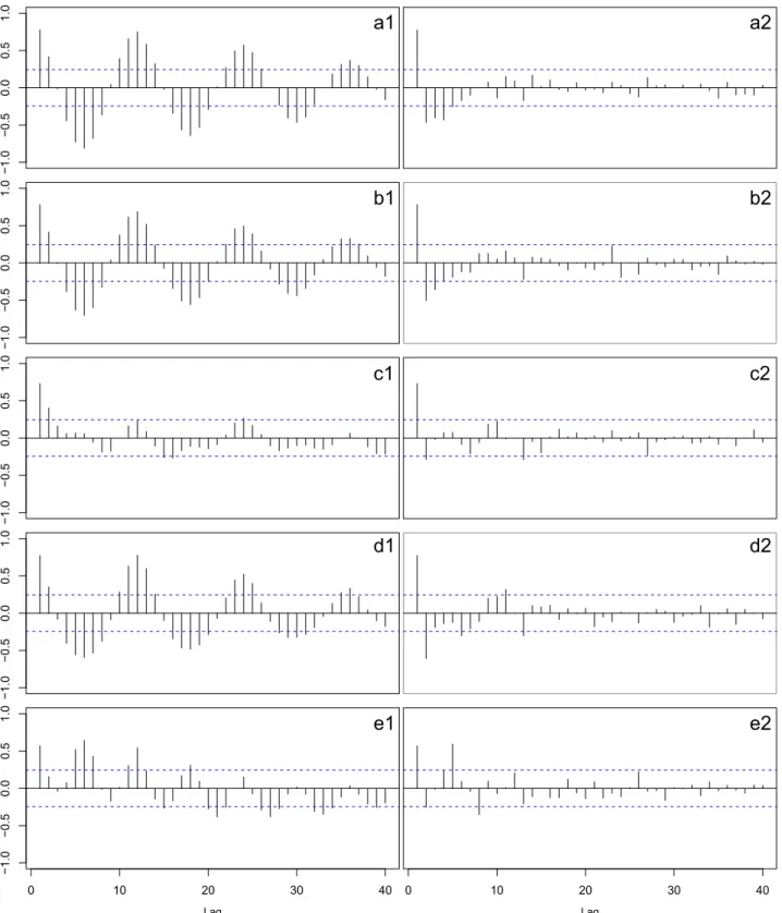
Fig. 2shows the sample ACF and the sample PACF for thefive retail series after transforming. It can be seen that in general the sample ACFs decay very slowly at regular lags and at multiples of seasonal period 12 and the sample PACFs have a large spike at lag 1 and cut off to zero after lag 2 or 3, suggesting that seasonal and/or or-dinary differencing might be necessary. For each retail series the Canova–Hanson test was applied for choosingD. After selectingD

successive KPSS tests were applied to determine the appropriate number of first differences. In the case of Boots, Booties and

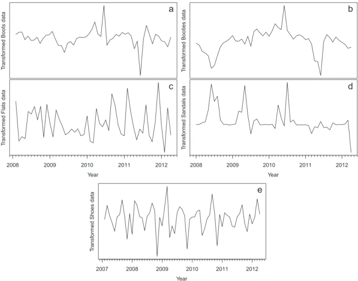
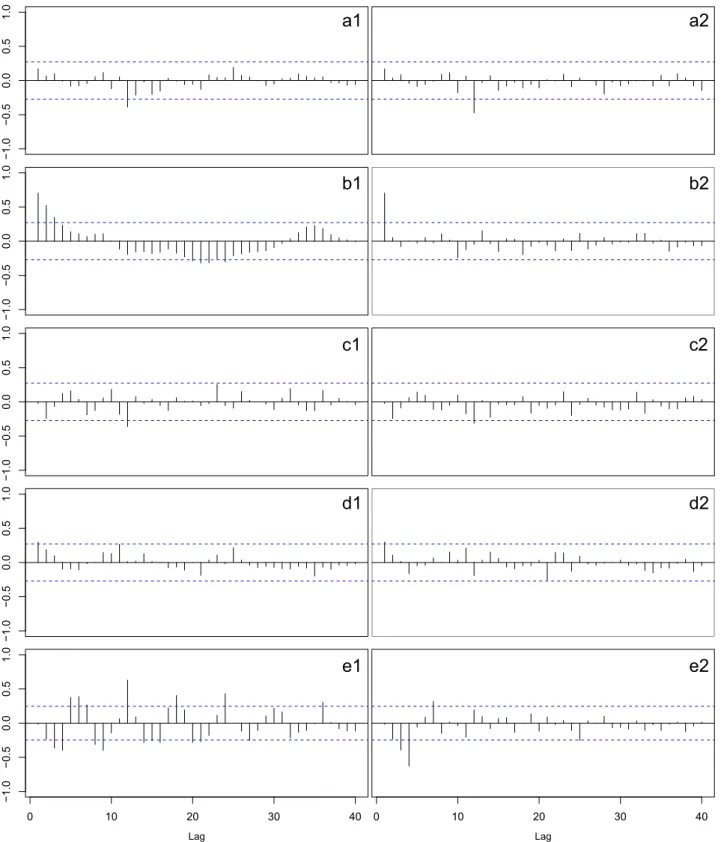
Sandals series one seasonal difference was required; in the case of Shoes series onefirst difference was required; and in the case of Flats series one seasonal difference and onefirst difference were required. The data of the five footwear categories after trans-forming and differencing are shown in Fig. 3. In all cases the transformation and the differencing have made the series look relatively stationary, as can be seen inFig. 4.

To be able to compare more accurately the forecasting

performance of both modeling approaches–ETS and ARIMA, for each time series we decided tofit, using the in-sample data from January 2007 to April 2011 (first 52 observations), all ARIMA

p d q P D Q

( , , )×( , , )mmodels wherepandqcould take values from

0 to 5, andP andQ could take values from 0 to 2. Usually the values of p q P, , and Q are not allowed to exceed these upper bounds to avoid problems with convergence or near-unit-roots

[24].

a1

a2

b1

b2

c1

c2

d1

d2

e1

e2

Fig. 2.Sample ACF (left panels) and sample PACF (right panels) plots for logged Boots data (a1, a2), logged Booties data (b1, b2), logged Flats data (c1, c2), Sandals data (d1, d2) and Shoes data (e1, e2).

4.2. Residual diagnostics

After identifying an appropriate model (ETS or ARIMA) we have to check whether the model assumptions are satisfied. The basic assumption for both models is that

ε

white noise process.

Hence, model diagnostic checking is accomplished through a careful analysis of the residuals:

(1) by constructing a histogram of the standardized residuals and comparing it with the standard normal distribution using the chi-square goodness of fit test, to check whether they are normally distributed;

(2) by examining the plot of the residuals to check whether the variance is constant;

(3) by computing the sample ACF and sample PACF of the re-siduals to see whether they do not form any pattern and are statistically insignificant, and by doing a Portmanteau test of the residuals–the more accurate is the Ljung–Box test[25]. The Ljung–Box test tests whether thefirstkautocorrelations of the residuals are significantly different from what would be expected from a white noise process. The null-hypothesis is that thosefirstkautocorrelations are null, so largep-values are indicative that the residuals are not distinguishable from a white noise series. Using the usual significance level of 5%, a model passes a Ljung–Box test if thep-value is greater than 0.05[30]. If there are significant spikes in sample ACF and/or in

sample PACF of the residuals or if the model fails a Ljung–Box test, another model should be tried; otherwise forecasts can be calculated.

4.3. Implementation

The time series analysis was carried out using the statistical software R programming language and the specialized package forecast[24,31].

For each retail series all admissible ETS models and all ARIMA

p d q P D Q

( , , )×( , , )mmodels wherepandqcould take values from

0 to 5, andPandQ could take values from 0 to 2 were applied using the in-sample period between January 2007 and April 2011 (_first 52 observations). The parameters of each model were esti-mated by maximizing the likelihood. The ETS model and the AR-IMA model with the minimum value of the AICc that passed the diagnostic checking were selected for forecasting. The Ljung–Box test was applied with a significance level of 5% based on thefirst 15 autocorrelations.

For each retail series, Table 1 gives the forecasting accuracy measures for in-sample data of the ETS model and ARIMA model selected according to the procedure described earlier. The forecast error measures presented in Table 1 are defined in Section 3.1. FromTable 1it can be observed that with the exception to Shoes series ARIMA models forecast better than ETS models in the training sample judged by the three most common performance

a

b

c

d

e

Fig. 3.Monthly sales of thefive footwear categories between January 2007 and April 2012 after transforming and differencing (a) seasonally differenced logged Boots data, (b) seasonally differenced logged Booties data, (c) doubled differenced logged Flats data, (d) seasonally differenced Sandals data and (e)first differenced Shoes data.

measures: RMSE, MAE and MAPE (with the single exception to MAPE for the Sandals series); although it should be emphasized that these results should not be used for forecast evaluation.

4.4. Cross-validation procedure

Since there is no universally agreed-upon performance mea-sure that can be applied to every forecasting situation, multiple

criteria are therefore often needed to give a comprehensive as-sessment of forecasting models[7]. The RMSE, MAE, and MAPE are the most commonly used forecast error measures among both academics and practitioners, and the retail forecasting literature is no exception[32].

For each retail series both selected models (ETS and ARIMA) were used to forecast on the out-of-sample period from May 2011 to April 2012 (12 observations). Both one-step and multiple-step

a1

a2

b1

b2

c1

c2

d1

d2

e1

e2

Fig. 4. Sample ACF (left panels) and sample PACF (right panels) plots for seasonally differenced logged Boots data (a1, a2), seasonally differenced logged Booties data (b1, b2), doubled differenced logged Flats data (c1, c2), seasonally differenced Sandals data (d1, d2) andfirst differenced Shoes data (e1, e2).

forecasts were produced. Using each modelfitted for the in-sam-ple period, point forecasts of the next 12 months (one-step fore-casts) and the forecast accuracy measures based on the errors obtained were computed. The values of RMSE, MAE and MAPE of one-step forecasts obtained are presented in Tables 2,3 and 4, respectively.

The cross-validation procedure for multi-step forecasts was based on a rolling forecasting origin modified to allow multi-step errors. Supposingnis the total number of observations,mis the in-sample size andhis the step-ahead, multi-step forecasts were obtained using the following algorithm:

For h¼1 to n-m For i¼1 to n-m-hþ1

Select the observation at time mþhþi-1 as out-of-sample

Use the observations until time mþi-1 to esti-mate the model

Compute the h-step error on the forecast for time mþhþi-1

Compute the forecast accuracy measures based on the errors obtained

In our case studym¼52 and n¼64. It should be emphasized that in multi-step forecasts the model is estimated recursively in each stepiusing the observations until timem+i−1.

Both one-step and multi-step forecasts are important in facil-itating a short and long planning and decision making. They si-mulate the real-world forecasting environment in which data need to be projected for short and long periods[3]. The values of RMSE, MAE and MAPE of multi-step forecasts obtained are presented in

Tables 2,3and4, respectively.

5. Results 5.1. Point forecasts

The results ofTables 2,3and4show that the overall out-of-sample forecasting performance of ETS and ARIMA models eval-uated via RMSE, MAE and MAPE is quite similar on both one-step and multi-step forecasts.

In one-step forecasts, ETS forecasts more accurately Flats and Shoes series than ARIMA, regardless of the forecast error measure considered. Improvements are of the order 20% or less. For Boots series the RMSE and MAE values of the ETS model are 33% and 40% smaller, respectively, but the MAPE value of the ARIMA model is 20% smaller. For Booties series the RMSE and MAE values of the

ARIMA model are 27% and 28% smaller, respectively, but the MAPE value of the ETS model is 15% smaller. For Sandals series the MAE and MAPE values of the ARIMA model are 4% and 59% smaller, respectively, but the RMSE value of the ETS model is 15% smaller. When considering each error measure individually over all time series in one-step forecasts ETS forecasts always more accu-rately than ARIMA: in four of the_five retail series (80%) for RMSE and in three of thefive retail series (60%) for MAE and MAPE.

In multi-step forecasts, ARIMA forecasts more accurately Booties series than ETS, regardless of the forecast error measure considered (with the exception to MAPE forh¼1 andh¼2 where improvements are, respectively, 16% and 7%). For Boots series ETS forecasts more accurately than ARIMA in 58% of the steps when considering RMSE and MAE (forh¼1–3, 8–11); ARIMA forecasts more accurately than ETS in 67% of the steps when considering MAPE (for h¼2–7,11,12). For Flats series ARIMA forecasts more accurately than ETS in 58% of the steps when considering RMSE (forh_¼2_–4,6_–8,12); ETS forecasts more accurately than ARIMA in 58% (forh¼1, 2, 5, 6, 9–11) and 83% (forh¼1, 2, 4–11) of the steps when considering MAE and MAPE, respectively. For Sandals series ETS forecasts more accurately than ARIMA in 92% (forh¼1–5, 7–

12) and 83% (for h¼2–5, 7–12) of the steps when considering RMSE and MAE, respectively; ARIMA forecasts more accurately than ETS in 58% of the steps when considering MAPE (forh¼2–8). For Shoes series ETS forecasts more accurately than ARIMA in 92% (forh¼1–9, 11, 12), 83% (forh¼1–8, 11, 12) and 75% (forh¼1–6, 8, 11, 12) of the steps when considering RMSE, MAE and MAPE, respectively.

When considering each error measure individually over all time series in multi-step forecasts ETS forecasts more accurately than ARIMA for RMSE and MAE: in three of the five retail series (60%) for RMSE and in four of thefive retail series (80%) for MAE. ARIMA forecasts more accurately than ETS for MAPE: in three of the _five retail series (60%). Overall ETS produces more accurate forecasts in 57% of the steps for RMSE and MAE and in 50% of the steps for MAPE.

These results also show that globally multi-step forecasts are better than one-step forecasts which is not surprising because multi-step forecasts incorporate information that is more updated. To see the individual point forecasting behavior we plotted the actual data versus the forecasts from both ETS and ARIMA models inFig. 5. In general, wefind that both ETS and ARIMA models have the capability to forecast the trend movement and seasonalfl uc-tuations fairly well. As expected, the exceptional increase in the sales offlats observed in March and April 2012 was not predicted by both models which under-forecasted the situation.

Table 1

Forecast accuracy measures for in-sample period (January 2007 to April 2011).

Retail series Model ME RMSE MAE MPE (%) MAPE (%)

Boots ETS(M, N, M) 254.43 1530.93 990.68 40.77 66.88 Log ARIMA(0, 0, 3)×(0, 1, 0)12 94.70 1320.60 722.54 19.48 33.66 Booties ETS(M, N, M) 88.46 384.61 255.36 23.72 51.67 Log ARIMA(1, 0, 0)×(0, 1, 2)12 47.01 290.22 170.75 10.94 29.04 Flats ETS(M, N, M) 4.16 284.67 192.14 6.07 24.56 Log ARIMA(0, 1, 0)×(0, 1, 1)12 21.61 174.19 122.01 0.26 20.33 ARIMA(1, 0, 0)×(0, 1, 0)12 450.11 1817.00 913.45 162.13 200.99 ARIMA(4, 1, 0)×(1, 0, 1)12 74.76 772.67 638.30 4.18 14.26

Table 2

RMSE for out-of-sample period forecasts (May 2011 to April 2012).

Retail series Model One-step forecasts Step-ahead of multi-step forecasts

1 2 3 4 5 6 7 8 9 10 11 12 Boots ETS 1263.63 1772.99 2424.99 2823.25 3629.93 4575.80 4913.38 3532.30 2012.93 812.90 203.37 181.60 193.94 ARIMA 1886.38 2315.46 2570.81 2866.74 2176.30 2307.08 2466.34 2269.76 2485.37 2657.74 1648.04 721.31 13.00 Booties ETS 1151.46 604.69 1056.24 1381.72 1733.74 2013.21 2074.64 1944.03 1418.13 665.95 384.70 59.27 87.77 ARIMA 843.68 538.86 719.85 943.74 1400.74 1594.39 1564.41 1141.17 671.83 131.48 53.90 19.49 14.57 Flats ETS 757.45 448.94 564.52 589.74 837.14 1048.20 1075.22 1218.73 1460.33 1682.60 1771.42 1909.65 1731.85 ARIMA 797.07 511.76 542.19 390.76 746.12 1049.51 1064.89 1152.75 1444.94 1719.01 1833.64 1944.21 1700.07 Sandals ETS 1201.01 1279.47 804.48 894.17 280.57 1413.19 2587.91 1200.82 1032.87 1434.66 1920.06 1722.84 1857.38 ARIMA 1414.50 1506.71 1475.93 1536.06 1608.02 1700.61 1788.28 1925.44 2110.13 2359.24 2724.48 3335.86 4657.98 Shoes ETS 651.72 624.38 738.61 628.96 732.80 904.56 962.67 827.87 949.67 1097.71 1220.35 1113.71 1178.26 ARIMA 798.62 876.86 1098.66 1103.78 1128.61 1121.56 1182.66 908.78 1058.72 1132.51 1212.91 1280.02 1236.24 Table 3

MAE for out-of-sample period forecasts (May 2011 to April 2012).

Retail series Model One-step forecasts Step-ahead of multi-step forecasts

1 2 3 4 5 6 7 8 9 10 11 12 Boots ETS 690.63 948.26 1342.31 1854.88 2356.78 3019.70 3584.63 2488.65 1650.09 560.31 148.10 167.65 193.94 ARIMA 1159.49 1257.29 1695.41 2115.84 1513.89 1676.37 1911.57 1660.83 1961.00 2045.75 1233.00 516.50 13.00 Booties ETS 749.78 357.31 756.01 1011.60 1318.99 1464.28 1500.68 1484.99 1087.02 539.72 286.58 49.74 87.77 ARIMA 539.75 324.15 526.36 677.33 972.66 1088.10 1018.14 836.41 481.61 106.55 47.65 19.48 14.57 Flats ETS 513.90 323.46 428.50 472.94 588.44 683.03 769.54 938.54 1152.01 1323.08 1489.38 1894.98 1731.85 ARIMA 601.65 369.83 448.94 337.28 503.29 715.21 782.96 916.03 1151.53 1376.13 1558.57 1928.18 1700.07 Sandals ETS 745.65 860.59 555.52 583.84 202.12 744.23 1042.48 548.40 527.79 747.01 1141.96 1350.99 1857.38 ARIMA 713.32 750.49 744.50 761.65 788.56 845.32 836.24 924.47 1108.91 1380.73 1836.12 2702.99 4657.98 Shoes ETS 547.97 475.31 553.71 447.48 496.22 669.36 762.33 618.28 664.29 889.93 1137.13 994.69 1178.26 ARIMA 683.03 666.59 831.30 854.60 838.40 835.83 868.51 634.15 804.72 876.07 1114.09 1129.78 1236.24 P. Ramos et al. / Robot ics and Computer -Integr ated Manufacturing 34 (20 1 5 ) 1 5 1 – 16 3

5.2. Forecast interval coverage

Producing estimates of uncertainty is an important aspect of forecasting which is often ignored. We also evaluated the perfor-mance of both forecasting methodologies in producing forecast intervals that usually provide coverages which are close to the nominal rates[23].Table 5shows the mean percentage of times that the nominal 95% and 80% forecast intervals contain the true

observations for both one-step and multiple-step forecasts. The results indicate that ETS and ARIMA models produce cov-erage probabilities that are close to the nominal rates for both one-step and multi-one-step forecasts. In one-one-step forecasts ARIMA slightly overestimates the coverage probabilities of both nominal forecast intervals. ETS slightly overestimates the coverage probability of the nominal 95% forecast interval and is equal to the coverage probability of the nominal 80% forecast interval. In multi-step Table 4

MAPE (%) for out-of-sample period forecasts (May 2011 to April 2012). Retail series Model One-step

forecasts

Step-ahead of multi-step forecasts

1 2 3 4 5 6 7 8 9 10 11 12 Boots ETS 211.03 130.02 199.10 100.39 67.97 70.70 74.97 61.63 63.42 32.13 12.96 103.58 340.24 ARIMA 169.87 176.39 198.09 63.76 53.31 53.77 61.13 54.30 64.78 77.86 82.96 87.64 22.81 Booties ETS 72.86 55.79 91.86 71.04 91.12 87.07 72.17 68.70 73.77 59.32 34.92 25.07 151.32 ARIMA 85.63 66.09 98.38 45.64 50.19 46.05 42.43 44.98 42.51 36.25 14.00 19.66 25.12 Flats ETS 49.26 31.28 43.12 46.75 43.27 42.45 48.15 61.59 63.09 58.49 53.49 62.32 54.15 ARIMA 62.37 33.43 49.39 45.49 44.04 46.10 50.87 63.78 64.82 63.15 57.09 63.40 53.16 Sandals ETS 165.87 449.07 253.55 231.13 246.04 281.16 298.73 321.29 114.01 26.76 40.64 44.24 54.33 ARIMA 68.55 1149.57 62.23 62.00 72.72 229.45 74.09 112.21 78.31 76.71 76.90 91.60 136.24 Shoes ETS 18.32 13.85 16.53 12.52 12.58 16.73 20.26 16.51 15.26 22.02 29.18 19.48 22.40 ARIMA 23.79 20.91 25.57 25.86 22.36 21.54 22.08 16.03 19.55 20.86 27.20 22.09 23.50

a

b

c

e

d

Fig. 5.Out-of-samplefixed forecasting comparison for the retail series (between May 2011 and April 2012): (a) pairs of Boots, (b) pairs of Booties, (c) pairs of Flats, (d) pairs of Sandals, and (e) pairs of Shoes.

forecasts, ETS underestimates the coverage probabilities of the nominal 95% forecast intervals in 92% of the steps and over-estimates in 8%. The coverage probabilities of the nominal 80% forecast intervals are underestimated in 83% of the steps and are equal to 80% in 17% of the steps. ARIMA underestimates the cov-erage probabilities of the nominal 95% forecast intervals in 67% of the steps, overestimates in 25% of the steps and is equal to 95% in 8% of the steps. The coverage probabilities of the nominal 80% forecast intervals are underestimated in 25% of the steps, over-estimated in 50% of the steps and are equal to 80% in 25% of the steps. The mean absolute deviation of the coverage probabilities generated by ETS is 14.7% for the nominal 95% forecast intervals and 12.1% for the nominal 80% forecast intervals. The mean ab-solute deviation of the coverage probabilities generated by ARIMA is 3.9% for the nominal 95% forecast intervals and 3.0% for the nominal 80% forecast intervals. So we may conclude from these results that in multi-step forecasts ETS tends to underestimate a little more the coverage probabilities of the forecast intervals than ARIMA.

5.3. Analysis and discussion

ETS and ARIMA models provide complementary approaches to the problem of time series forecasting. While the former frame-work is based on a description of trend and seasonality in the data, the latter one aims to describe the autocorrelations in the data. There is the idea that ARIMA models are more general than ex-ponential smoothing models. Actually, the two classes of models are complimentary each with its strengths and weaknesses. While linear exponential smoothing models are all special cases of AR-IMA models, the non-linear exponential smoothing models have no equivalent ARIMA counterparts. There are also many ARIMA models which have no exponential smoothing counterparts. In particular, every ETS model is non-stationary while ARIMA models can be stationary.

It may also be thought that ARIMA is advantageous over ETS because it is a larger model class. However, the results in[5]show that the exponential smoothing models performed better than the ARIMA models for the seasonal M3 competition data. (For the annual M3 data, the ARIMA models performed better.) In a dis-cussion of these results, Hyndman and Athanasopoulos [15]

speculate that the larger model space of ARIMA models actually harms forecasting performance because it introduces additional uncertainty and that the smaller exponential smoothing class is sufficiently rich to capture the dynamics of almost all real business and economic time series.

Our results reinforce the idea that ARIMA models do not pro-duce more accurate forecasts than state space models when an automatic forecasting algorithm is applied. And that state space models can be very competitive in producing automatic forecasts of univariate time series which are often needed in any retail business. In fact state space models seem to have a slightly better performance than ARIMA models in the presence of a larger vo-latility in the case of one-step forecasts, as showed the

out-of-sample results of Flats and Shoes series. In the case of multi-step forecasts that is not so evident and globally their performance is quite similar. Our results also indicate that ETS and ARIMA models produce coverage probabilities that are close to the nominal rates for one-step forecasts. In multi-step forecasts ETS tends to un-derestimate a little more the coverage probabilities of the forecast intervals than ARIMA.

We also concluded that globally ARIMAfits the data better than ETS but that does not mean that it forecasts better. In fact, a model whichfits the data better does not necessarily forecast better, and the_fit error measures should not be used as a way to select a model for forecast[19].

As mentioned inSection 3.1, one of the limitations of the MAPE is having huge values when data contain very small numbers. The large values of MAPE of both models for the Boots, Booties and Sandals retail series are explained by the fact that during the out-of-sample period there are some months with almost no sales (close to zero).

In general, wefind that both ETS and ARIMA models have the capability to forecast the trend movement and seasonalfl uctua-tions fairly well. As expected, the exceptional increase in the sales offlats observed in March and April 2012 was not predicted by both models which under-forecasted the situation.

6. Conclusions and future work

Accurate retail sales forecasting can have a great impact on effective management of retail operations. Retail sales time series often exhibit strong trend and seasonal variations presenting challenges in developing effective forecasting models. How to ef-fectively model these series and how to improve the quality of forecasts are still outstanding questions. Despite the investigator's efforts, the several existing studies have not led to a consensus about the relative forecasting performances of ETS and ARIMA modeling frameworks when they are applied to retail sales data.

The purpose of this work was to compare the forecasting per-formance of ETS and ARIMA models when applied to a case study of retail sales offive different categories of women footwear from the Portuguese retailer Foreva. As far as we know it is the_first time ETS models are tested for retail sales forecasting.

For each retail series all admissible ETS models were applied using the in-sample period. To identify an appropriate ARIMA model for each retail series, after deciding the required transfor-mations for variance stabilization, unit-root tests were applied to select the necessary degrees of differencing to achieve stationarity. To be able to compare more accurately the forecasting perfor-mance of both modeling approaches, for each time series we decided tofit all the ARIMA models where pand q could take values from 0 to 5, andPandQcould take values from 0 to 2. The ETS model and the ARIMA model with the minimum value of the AICc that passed the diagnostic checking were selected for fore-casting on the out-of-sample.

Both one-step and multiple-step forecasts were produced using Table 5

Forecast interval coverage for out-of-sample period forecasts (May 2011 to April 2012). Model Nominal coverage (%) One-step forecasts Step-ahead of multi-step forecasts

1 2 3 4 5 6 7 8 9 10 11 12

ETS 95 96.8 84.8 80.2 82.0 78.0 75.2 68.6 63.4 80.0 85.0 86.6 90.0 100.0

80 80.0 68.2 60.2 58.0 69.0 67.6 63.0 63.4 60.0 75.0 80.0 70.0 80.0

ARIMA 95 95.2 88.4 85.6 92.0 95.6 92.8 94.4 96.6 96.0 95.0 93.4 90.0 80.0

the selected models. The results show that the overall out-of-sample forecasting performance of ETS and ARIMA models eval-uated via RMSE, MAE and MAPE is quite similar on both one-step and multi-step forecasts. On both modeling approaches multi-step forecasts are generally better than one-step forecasts which is not surprising because multi-step forecasts incorporate information that is more updated. The performance of both forecasting methodologies in producing forecast intervals that provide cov-erages which are close to the nominal rates was also evaluated. The results indicate that both ETS and ARIMA produce coverage probabilities that are very close to the nominal rates. ARIMA being a larger model class it could be thought to be advantageous over ETS. Our results show that when an automatic algorithm is applied the overall out-of-sample forecasting performance of ARIMA models is not better than ETS models in predicting retail sales, and neither is best for all circumstances.

Retailers are increasing their assortments in response to con-sumer demands for higher product variety. The new paradigm of mass customization is forcing manufacturers to redesign and change products constantly[33–35]. As a consequence, products life cycles have been decreasing making sales at the SKU (Stock Keeping Unit) level in a particular store difficult to forecast, as time series for these products tend to be short. Moreover, retailers are increasing marketing activities such as price reductions and pro-motions due to more intense competition and recent economic recession. Products are typically on promotion for a limited period of time, e.g. 1 week, during which demand is usually substantially higher occurring many stock-outs due to inaccurate forecasts[36]. Stock-outs can be very negative to the business because these lead to dissatisfied customers. How to balance the loss due to stock-outs and the cost of safety stocks is clearly an important issue for today's retailers.

Acknowledgments

Project “NORTE-07-0124-FEDER-000057” is financed by the North Portugal Regional Operational Programme (ON.2 - O Novo Norte), under the National Strategic Reference Framework (NSRF), through the European Regional Development Fund (ERDF), and by national funds, through the Portuguese Funding Agency, Fundação para a Ciência e a Tecnologia (FCT).

References

[1]X. Zhao, J. Xie, R.S.M. Lau, Improving the supply chain performance: use of forecasting models versus early order commitments, Int. J. Prod. Res. 39 (17) (2001) 3923–3939.

[2]P. Doganis, E. Aggelogiannaki, H. Sarimveis, A combined model predictive control and time series forecasting framework for production–inventory sys-tems, Int. J. Prod. Res. 46 (24) (2008) 6841–6853.

[3]I. Alon, Q. Min, R.J. Sadowski, Forecasting aggregate retail sales: a comparison of artificial neural networks and traditional method, J. Retail. Consum. Serv. 8 (3) (2001) 147–156.

[4]G. Box, G. Jenkins, G. Reinsel, Time Series Analysis, 4th edition, Wiley, NJ, 2008. [5]R.J. Hyndman, A.B. Koehler, J.K. Ord, R.D. Snyder, Forecasting with Exponential

Smoothing: The State Space Approach, Springer-Verlag, Berlin, 2008. [6]I. Alon, Forecasting aggregate retail sales: the winters' model revisited, in: J.

C. Goodale (Ed.), The 1997 Annual Proceedings, Midwest Decision Science Institute, 1997, pp. 234–236.

[7]C.W. Chu, P.G.Q. Zhang, A comparative study of linear and nonlinear models for aggregate retail sales forecasting, Int. J. Prod. Econ. 86 (2003) 217–231. [8]C. Frank, A. Garg, L. Sztandera, A. Raheja, Forecasting women's apparel sales

using mathematical modeling, Int. J. Cloth. Sci. Technol. 15 (2) (2013) 107–125. [9]G. Zhang, M. Qi, Neural network forecasting for seasonal and trend time series,

Eur. J. Oper. Res. 160 (2005) 501–514.

[10] J. Kuvulmaz, S. Usanmaz, S.N. Engin, Time-series forecasting by means of linear and nonlinear models, in: Advances in Artificial Intelligence, 2005. [11] L. Aburto, R. Weber, Improved supply chain management based on hybrid

demand forecasts, Appl. Soft Comput. 7 (1) (2007) 126–144.

[12]K.F. Au, T.M. Choi, Y. Yu, Fashion retail forecasting by evolutionary neural networks, Int. J. Prod. Econ. 114 (2) (2008) 615–630.

[13]W.K. Wong, Z.X. Guo, A hybrid intelligent model for medium-term sales forecasting in fashion retail supply chains using extreme learning machine and harmony search algorithm, Int. J. Prod. Econ. 128 (2010) 614–624. [14] Y. Pan, T. Pohlen, S. Manago, Hybrid neural network model in forecasting

aggregate U.S. retail sales, in: Advances in Business and Management Fore-casting, vol. 9, 2013, pp. 153–170.

[15] R.J. Hyndman, G. Athanasopoulos, Forecasting: Principles and Practice, Online Open-access Textbooks,〈http://otexts.com/fpp/〉, 2013.

[16]S. Arlot, C. Alain, A survey of cross-validation procedures for model selection, Stat. Surv. 4 (2010) 40–79.

[17] D. Pena, G.C. Tiao, R.S. Tsay, A Course in Time Series Analysis, John Wiley & Sons, New York, 2001.

[18]E.S. Gardner, Exponential smoothing: the state of the art, J. Forecast. 4 (1) (1985) 1–28.

[19]S. Makridakis, S. Wheelwright, R. Hyndman, Forecasting: Methods and Ap-plications, 3rd edition, John Wiley & Sons, New York, 1998.

[20] E.S. Gardner, Exponential smoothing: the state of the art—Part II, Int. J. Fore-cast. 22 (4) (2006) 637–666.

[21]M. Aoki, State Space Modeling of Time Series, Springer-Verlag, Berlin, 1987. [22] P.J. Brockwell, R.A. Davis, Introduction to Time Series and Forecasting, 2nd

edition, Springer-Verlag, New York, 2002.

[23] R.H. Shumway, D.S. Stoffer, Time Series Analysis and its Applications: With R Examples, 3rd edition, Springer, New York, 2011.

[24] R.J. Hyndman, Forecast: Forecasting Functions for Time Series. R Package Version 4.06,〈http://cran.rstudio.com/〉, 2008.

[25] W.S. Wei, Time Series Analysis: Univariate and Multivariate Methods, 2nd edition, Addison Wesley, 2005.

[26] J.D. Cryer, K.S. Chan, Time Series Analysis with Applications in R, Springer, 2009.

[27] F. Canova, B.E. Hansen, Are seasonal patterns constant over time? A test for seasonal stability, J. Bus. Econ. Stat. 13 (1985) 237–252.

[28] D. Kwiatkowski, P.C. Phillips, P. Schmidt, Y. Shin, Testing the null hypothesis of stationary against the alternative of a unit root, J. Econom. 54 (1992) 159–178. [29] M. Stone, An asymptotic equivalence of choice of model by cross-validation

and Akaike's criterion, J. R. Stat. Soc. Ser. B Methodol. 39 (1) (1977) 44–47. [30] G.M. Ljung, G.E.P. Box, On a measure of lack offit in time series models,

Biometrika 65 (1978) 297–303.

[31] R Development Core Team. R: A Language and Environment for Statistical Computing. R Version 3.0.0,〈http://www.R-project.org/〉, 2013.

[32] R.A. Fildes, P. Goodwin, Against your better judgment? How organizations can improve their use of management judgment in forecasting, Interfaces 37 (2007) 570–576.

[33] D. Mourtzis, M. Doukas, F. Psarommatis, Design and operation of manu-facturing networks for mass customisation, CIRP Ann. Manuf. Technol. 63 (1) (2013) 467–470.

[34] D. Mourtzis, M. Doukas, F. Psarommatis, A multi-criteria evaluation of cen-tralized and decencen-tralized production networks in a highly customer-driven environment, CIRP Ann. Manuf. Technol. 61 (1) (2012) 427–430.

[35] A.J. Dietrich, S. Kirn, V. Sugumaran, A service-oriented architecture for mass customization—a shoe industry case study, IEEE Trans. Eng. Manag. 54 (1) (2007) 190–204.

[36] O.G. Ali, S. Sayin, T. vanWoensel, J. Fransoo, Sku demand forecasting in the presence of promotions, Expert Syst. Appl. 36 (10) (2009) 12340–12348.