EVALUATION OF TRAFFIC INPUT LEVELS FOR PAVEMENT ME DESIGN
By
JUNXIANG LOU
Bachelor of Science in Civil Engineering Southwest Jiaotong University
Chengdu, Sichuan 2012
Submitted to the Faculty of the Graduate College of the Oklahoma State University
in partial fulfillment of the requirements for
the Degree of MASTER OF SCIENCE
ii
EVALUATION OF TRAFFIC INPUT LEVELS FOR PAVEMENT ME DESIGN Thesis Approved: Kelvin C.P. Wang Thesis Adviser M. Tyler Ley Stephen A. Cross
iii Name: JUNXIANG LOU
Date of Degree: DECEMBER, 2014
Title of Study: EVALUATION OF TRAFFIC INPUT LEVELS FOR PAVEMENT ME DESIGN
Major Field: CIVIL ENGINEERING
ABSTRACT: Traffic loads are one of the key data elements required for the design and analysis of pavement structures. The MEPDG requires full axle-load spectrum mainly based on continuous site-specific Weigh-In-Motion (WIM) data sets for each axle type and axle-load group. Due to the fact that collecting high quality WIM data is expensive, challenging and analyzing them requires extensive efforts and expertise, many state DOTs have to rely on traffic data from various acquisition technologies and length of time coverage for the implementation of MEPDG. This paper studies the impacts and variability of various traffic data collection efforts on MEPDG predicted performance. Twelve traffic data input scenarios are simulated to consider various traffic data collection efforts at 20 WIM sites in Oklahoma. A total of 1,440 MEPDG runs are performed with 3 AADTT levels, and 2 growth rates. The impacts of traffic load level, WIM data coverage, vehicle distribution, axle loading, and using regional and national defaults on predicted pavement performance are evaluated. This study has recommended the minimum required traffic data collection efforts for highway agencies to prepare traffic data for the implementation of MEPDG.
iv TABLE OF CONTENTS Chapter Page ABSTRACT ... iii I. INTRODUCTION ... 1 Background ... 1 Literature Review... 5 Problem Statement ... 7 Research Objective ... 7 II. METHODOLOGY ... 9 Scope of Work ... 9
Pavement Structure Design ... 10
Step 1: Locating WIM Stations... 10
Step 2: Determining Division and County For Each Site ... 15
Step 3: Obtaining Soil Data ... 16
Step 4: Designing Pavement Thickness ... 19
Simulated Traffic Input Scenarios ... 19
Data Sources ... 19
Traffic Input Scenarios ... 21
Other Inputs for MEPDG ... 30
AADTT & Traffic Growth Rate ... 30
Operating Speed ... 30
Axle per Truck ... 30
Climate ... 30
Percent of Truck In Design Lane ... 32
v
Chapter Page
III. MEPDG RESULTS ANALYSIS ... 33
MEPDG Pavement Performance ... 33
Impact of Traffic Level ... 33
Impact of WIM Data Coverage ... 39
Impact of Vehicle Distribution ... 42
Use of Regional and National Defaults ... 45
Impact of Axle Loading ... 48
IV. DISCUSSIONS... 52
V. CONCLUSIONS ... 59
vi
LIST OF TABLES
Table Page
Table 2.1 WIM Stations In Oklahoma ...11
Table 2.2 GPS Coordinates of WIM Stations in Oklahoma ...13
Table 2.3 Division and County of WIM Sites ...17
Table 2.4 1993 AASHTO Pavement Design Results ...20
Table 2.5 48-hour VCD and TTC Class ...25
Table 2.6 Aggregation Class for Traffic Inputs in Kentucky Transportation Cabinet (KYTC) ...26
Table 2.7 Damage Caused By Each Axle Type ...27
Table 2.8 Statewide and MEPDG Default “Axles per Truck” ...31
vii
LIST OF FIGURES
Figure Page
Figure 1.1 Simplified Inner Process of MEPDG ...1
Figure 2.1 Locating WIM Site Manually ...12
Figure 2.2 Plot of WIM Sites In Oklahoma ...14
Figure 2.3 Divisions and County of Oklahoma ...15
Figure 2.4 Determining County of The Sample WIM Site ...16
Figure 2.5 Geologic Unit And Soil Classification of Sample WIM Site ...18
Figure 2.6 Determining Number of Clusters ...28
Figure 2.7a Three Levels of Loading Group ...29
Figure 3.1a Pavement Performance (Long. Crack) at Various Traffic Levels ...34
Figure 3.1b Pavement Performance (Alligator Crack) at Various Traffic Levels ...34
Figure 3.1c Pavement Performance (Rutting) at Various Traffic Levels ...35
Figure 3.1d Pavement Performance (IRI) at Various Traffic Levels ...35
Figure 3.2a Pavement Performance Changes (Long. Crack) at Various Traffic Levels ...37
Figure 3.2b Pavement Performance Changes (Alligator Crack) at Various Traffic Levels ...37
Figure 3.2c Pavement Performance Changes (Rutting) at Various Traffic Levels ...38
Figure 3.2d Pavement Performance Changes (IRI) at Various Traffic Levels ...38
Figure 3.3a Predicted Pavement Performance Changes (IRI) with Various WIM Data Coverage (Scenarios 1, 2, 3) ...40
Figure 3.3b Predicted Pavement Performance Changes (Rutting) with Various WIM Data Coverage (Scenarios 1, 2, 3) ...40
Figure 3.3c Predicted Pavement Performance (IRI) with Various WIM Data Coverage (Scenarios 1, 2, 3) ...41
viii
Figure Page
Figure 3.3d Predicted Pavement Performance (Rutting) with Various WIM Data
Coverage (Scenarios 1, 2, 3) ...41
Figure 3.4a Predicted Pavement Performance Changes (IRI) with Various Classification Data Coverage (Scenarios 4, 5, 6) ...43
Figure 3.4b Predicted Pavement Performance Changes (Rutting) with Various Classification Data Coverage (Scenarios 4, 5, 6) ...43
Figure 3.4c Predicted Pavement Performance (IRI) with Various Classification Data Coverage (Scenarios 4, 5, 6) ...44
Figure 3.4d Predicted Pavement Performance Changes (Rutting) with Various Classification Data Coverage (Scenarios 4, 5, 6) ...44
Figure 3.5a Predicted Pavement Performance Changes (IRI) with Regional/National Traffic Defaults (Scenarios 7, 8, 9) ...46
Figure 3.5b Predicted Pavement Performance Changes (Rutting) with Regional/National Traffic Defaults (Scenarios 7, 8, 9) ...46
Figure 3.5c Predicted Pavement Performance (IRI) with Regional/National Traffic Defaults (Scenarios 7, 8, 9) ...47
Figure 3.5d Predicted Pavement Performance (Rutting) with Regional/National Traffic Defaults (Scenarios 7, 8, 9) ...47
Figure 3.6a Predicted Pavement Performance Changes (IRI) with Various Axle Loading Methods (Scenarios 10, 11, 12) ...49
Figure 3.6b Predicted Pavement Performance Changes (Rutting) with Various Axle Loading Methods (Scenarios 10, 11, 12) ...50
Figure 3.6c Predicted Pavement Performance (IRI) with Various Axle Loading Methods (Scenarios 10, 11, 12) ...50
Figure 3.6d Predicted Pavement Performance (Rutting) with Various Axle Loading Methods (Scenarios 10, 11, 12) ...51
Figure 4.1a VCD For WIM 2 ...53
Figure 4.1b VCD for WIM 29 ...53
Figure 4.2a Tandem Axle Loading for WIM 2 ...55
Figure 4.2b Tandem Axle Loading for WIM 29...55
Figure 4.3a MAF (Class 5 Vehicle) for WIM 2...57
Figure 4.3b MAF (Class 5 Vehicle) for WIM 29 ...57
ix
Figure Page
1 CHAPTER I
INTRODUCTION Background
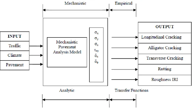
MEPDG is the new generation of pavement design and analysis software, a simplified inner process of MEPDG is shown in Figure 1.1.
Figure 1.1 Simplified Inner Process of MEPDG
Using mechanics, inputs are first transferred into stress and strain, and then the
2
Among all these inputs, traffic is one of the key elements required for the structural design/analysis of pavement structures. Instead of using Equivalent Single Axle Load (ESAL) in the 1993 AASHTO Design Guide to characterize traffic throughout the
pavement design life (1), the mechanistic pavement damage computations in the MEPDG requires axle-load spectra (2), defined as the number of axle passes by load level and axle configuration. In practice, highway agencies typically collect three types of traffic data: weigh-in-motion (WIM), automatic vehicle classification (AVC), and vehicle counts.
Weigh-In-Motion, defined in ASTM, is the process of measuring the dynamic tire forces of a moving vehicle and estimating the corresponding tire loads of the static vehicle (ASTM, 2002), and therefore estimating a moving vehicle’s gross weight and the portion of that weight that is carried by each wheel, axle, or axle group, or combination. The information is critical for highway management, traffic operation and control, and structural design of pavements and bridges.
A WIM system usually consists of weight sensors, inductive loop detectors, and a computer interface in a roadside cabinet. Depending on applications, optional peripheral devices can include Automatic Vehicles Identification (AVI) interfaces, video cameras, and modems. Weight sensors are the key hardware in the system. These sensors can be portable or permanently installed depending on system requirements. There are three basic classes of WIM sensors: piezoelectric sensors, bending plates, and load cells. Inductive loop detectors are used to detect approaching vehicles and measure axle
spacing and vehicle speed. The computer interface is usually a data logger equipped with a microprocessor. It monitors and stores the traffic flow data that can be either retrieved on site or transmitted wirelessly from a remote location to a central office. The American
3
Society for Testing and Materials (ASTM) classifies WIM systems as Type I, II, III, or IV. This classification is based on speed ranges, data gathering capabilities, and intended applications.
AVC system identifies vehicle class as it passes through a series of detection devices. T Kon et al. (26) summarized that majority technologies relevant to vehicle detection include loop detectors, infrared, ultrasonic, microwave and video detectors.
Loop detectors are the most widely used technology for vehicle detection in the United States. A loop detector consists of one or more loops of wire embedded in the pavement and connected to a control box. The loop may be excited by a signal ranging in frequency from 10 kHz to 200 kHz. This loop forms an inductive element in combination with the control box. When a vehicle passes over or rests on the loop, the inductance of the loop is reduced. This causes a detection to be signaled in the control box.
There are two types of infrared (IR) detectors, active and passive. In both types of detectors the LED or laser diode illuminates the target, and the reflected energy is focused onto a detector consisting of a pixel or an array of pixels. The measured data is then processed using various signal-processing algorithms to extract the desired
information on count, presence, speed, and occupancy data in both night and day operation. The laser diode type can also be used for vehicle classification because it provides vehicle profile and shape data.
Ultrasonic detectors have not become widely used in the United States, but they are very widely used in Japan in traffic applications with two types of sensors: presence-only and speed measuring. Both types operate by transmitting ultrasonic energy and measuring the
4
energy reflected by the target for measurements of vehicle presence, speed, and occupancy. Microwave detectors have been used extensively in Europe, but not in the United States, by measuring the energy reflected from target vehicles within the field of view to measure speed, occupancy, and presence.
A video image processor (VIP) is a combination of hardware and software which extracts desired information from data provided by an imaging sensor to detect speed, occupancy, count, and presence.
Comparing to the WIM and AVC methods, traffic counts has the least information of traffic, and only record AADT (Annual Average Daily Traffic). Many DOTs use this kind of data to build state traffic counts map or interactive live traffic map.
Among the three types of traffic data gathering, only WIM data is able to generate both truck classification and axle loading spectra data required in MEPDG. However,
collecting high quality WIM data is expensive, and analyzing the data requires extensive efforts and expertise. Many state DOTs have to utilize traffic data from various collection techniques. Moreover, data coverage of traffic data acquisition systems can vary widely from continuously operating to simple 48-hour (or less) data coverage. Even for
continuously operating data acquisition systems; however, data coverage time may be hampered by system malfunctions. Therefore, there is need to learn how the variations of traffic data impact the outcome and implementation of MEPDG.
5 Literature Review
Various methodologies have been developed to obtain traffic data input and the data variability on pavement design and performance.
Extensive one-at-a-time (OAT) analyses have been performed to investigate the
sensitivity of MEPDG inputs on pavement performance (3). It is found that main distress of both flexible and rigid pavement was sensitive or very sensitive to traffic volume.
Cooper et al. (4) evaluated the sensitivity of three traffic levels considering five pavement structures and the combinational interaction effects of the input parameters and
concluded that traffic level was the main influencing factor for pavement distress.
Li et al. (5) performed comprehensive sensitivity analysis using Washington DOT (WSDOT) WIM data. For typical WSDOT pavement design, axle load spectra inputs showed moderate sensitivity to pavement performance.
Based on the comparisons of MEPDG predictions with field observations for rigid
pavements in Kansan DOT, Khanum et al. (6 and 7) found that IRI was the most sensitive output with respect to the traffic inputs, followed by the percentage of cracked slabs.
Sauber et al. (8) examined the differences of pavement performance using Level 1 site-specific data and Level 3 MEPDG defaults. Distress predictions were found to be significant different.
Using Arkansas statewide averages and MEPDG default axle load spectra, Tran, Nam H et al. observed significant differences in predicted pavement performance (9).
6
North Carolina DOT conducted clustering analysis on traffic load spectra and found that 99% of the pavement damage was due to single axle and tandem axle repetitions (10).
Ritchie and Hallenbeck (11) studied the relationship between data collection sampling efforts and the accuracy in estimating the average annual daily traffic (AADT). The accuracy in predicting AADT increases with the number of days used in establishing the mean.
The 2001 TMG recommends collecting traffic volume data through a combination of a limited number of continuously operating reference systems and a larger number of shorter duration coverage systems (12).
Using Long-Term Pavement Performance (LTPP) WIM data sets, Papagiannakis et al. (13) established the minimum traffic data collection effort required for pavement design applications considering simulated traffic data collection scenarios.
Selezneva et al. (14) investigated the effect of bias in weigh-in-motion (WIM) axle weight measurements. It was found that drift in WIM system calibration leading to a more than 5% bias in mean error between true and WIM-measured axle weight could lead to significant differences in MEPDG design outcomes.
Realizing that it is not always practical to obtain site specific traffic data, Abbas and Frankhouser (15) evaluated the MEPDG outcomes calculated from continuous traffic monitoring data from Ohio DOT, generated site-specific and statewide traffic inputs. It is recommended to estimate the AADTT and the vehicle class distribution from
site-specific short-term or continuous counts and obtain the truck growth rate from ODOT Modeling and Forecasting Section. Other traffic inputs like hourly distribution factors,
7
axle load spectra, and number of axles per truck, state wide traffic data could be applied. MEPDG defaults can be used for the monthly adjustment factors.
McCracken et al. (16) observed a significant difference between the design result of 1993 American Association of State Highway and Transportation Officials (AASHTO) Design Guide and the Mechanistic Empirical Pavement Design Guide (MEPDG). Also, it is found that the MEPDG outcomes of different levels of inputs (typical value, correlated value or measured value) could lead to two inches of difference in design thickness.
Problem Statement
Despite these presented past research efforts, the challenge remains to determine the combination of traffic data acquisition technology and the time coverage required for particular pavement design situations. A lot of previous research focus on AADTT and traffic growth rate levels or the most sensitive factor that affects a certain kind of pavement distress, only a few of them compare the distress predicted with site specific data with statewide average value or MEPDG default while data time coverage has never been taken into consideration. This issue needs to be addressed in light of the sensitivity of the pavement design and performance analysis to the level of traffic data input.
Research Objective
In this paper, a comprehensive approach is proposed to establish the relationship between traffic data collection efforts (combination of traffic data acquisition technologies and length of time coverage) and the variability on predicted pavement performance using
8
MEPDG. Twelve traffic data input scenarios are simulated to use (1) data typically collected by permanent WIM systems and other technologies, such as portable WIM, automated vehicle classification (AVC) and short-term truck counts; (2) continuous coverage for axle loads, classification, or counts, while others involved discontinuous data coverage. A total of 20 flexible pavement sites at locations where WIM are installed for Oklahoma are analyzed to predict pavement performance using MEPDG. The
sections have wide distribution of average annual daily truck traffic (AADTT) volumes and structural thicknesses. Addition analysis considering three levels of AADTT and two levels of annual growth rate are conducted to examine their effects on pavement
9 CHAPTER II
METHODOLOGY Scope of Work
The scope of this study is to investigate the sensitivity of traffic inputs on flexible pavement performance. Flexible pavement structures in the study are designed using the 1993 AASHTO Pavement Design Guide (1) at the 20 WIM locations in Oklahoma. The design results are input into MEPDG for distress predicting and further analysis. MEPDG requires the following inputs (2):
Structure
Thickness of each pavement layer
Property of materials been used in each layer, including modulus of subgrade and aggregate, sieve analysis results etc.
Traffic
The base year traffic volume. One important input in this category is annual average daily truck traffic (AADTT).
Volume adjustment factors. The base year AADTT must be adjusted by monthly distribution, hourly distribution, vehicle class distribution (VCD), and traffic growth factors. These factors can be determined on the basis of classification counts obtained from WIM, AVC, or vehicle count data.
10
Axle load distribution factors (axle load spectra). The axle load distribution factors represent the percentage of the total axle applications within each load Interval for a specific axle type (single, tandem, tridem, and quad) and truck class (class 4 to class 13). The axle load distributions or spectra can be determined only from WIM data.
General traffic inputs, such as number of axles per truck, axle configuration, and wheel base. These data are used in the calculation of traffic loading for
determining pavement responses. The default values provided for the general traffic inputs are recommended if more accurate data are not available. Climate
Climate includes temperature, altitude, ground water level etc.
In this chapter, pavement structure design based on 1993 AASHTO Guide at the
Oklahoma WIM stations, development of the 12 simulated traffic input scenarios, other inputs for MEPDG and MEPDG predicted pavement performance results are addressed in details.
Pavement Structure Design
The process of design pavement structure in this study is divided into 4 steps: locating WIM stations, determining ODOT Division and County for each design site, obtaining soil data and designing pavement thickness based on 1993 AASHTO Guide.
Step 1: Locating WIM Stations
There are 23 operating permanent WIM stations within the state of Oklahoma (20). The location of these WIM stations is shown in Table 2.1.
11
Table 2.1 WIM Stations In Oklahoma WIM ID Func Class Sensor County FIPS Route # Location
1 2 P 74 75 6.3 miles south of Jt. US-60 2 1 P 50 35 2.6 miles south of Jt. SH-7 3 11 P 55 240 2.57 miles West of Jt. I-35
5 2 P 73 69 6.4 miles south Jt. US-412
6 1 P 54 40 1.0 miles west of Jt. US-75 south
7 2 P 6 270 2.7 miles west of Jt. SH-8
8 2 P 67 99 0.3 Miles North Jt. SH-59 West
9 2 P 62 3 1.1 miles East of Jt. SH-1
10 2 P 61 69 3.75 Miles North Jt. SH-113 11 6 P 26 81 2.46 Miles South Jt. US-81bus South
16 2 P 49 412 2.6 Miles West Jt. US-69
21 7 P 40 69 1.10 miles north of the Red River Bridge
22 7 P 40 112 1.2 miles East Jt. US-59
23 2 P 47 412 2.2 miles West Jt. US-58
25 2 P 287 5.6 miles north of intersect of SH-3 & US 287
27 1 P 36 35 2.5 Miles North Jt. US-60
28 1 P 9 40 Location Not set as of 10/21/02 29 1 P 68 40 0.5 Miles East Mile Marker 311 30 1 P 44 35 100 Ft. North of Mile Marker 105 32 2 P 70 3.5 miles West of Junction US-259/US-70 104 1 P 42 35 0.5 miles North of Jt. Waterloo Rd 114 1 P 75 40 0.1 Miles West of Mile Marker 43 118 2 P 16 62 1.3 Miles West Jt. SH-115
12
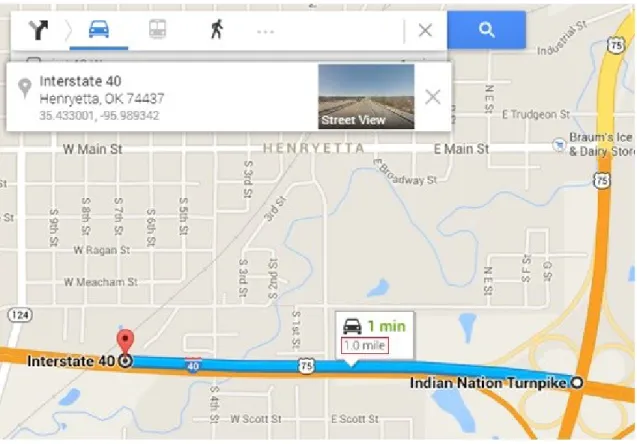
However, no GPS coordinates are provided. With the assistance of Google Map, the GPS locations of the 23 WIM sites are located (Figure 2.1 is an example of WIM 6).
Figure 2.1 Locating WIM Site
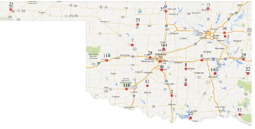
GPS Coordinates of 23 WIM Stations and a plot of WIM site distribution are obtained and shown in Table 2.2 and Figure 2.2 respectively.
13
Table2.2 GPS Coordinates of WIM Stations in Oklahoma WIM Latitude Longitude
1 36.8204 -95.935386 2 33.460727 -97.144922 3 35.391499 -97.541317 5 36.077771 -95.364831 6 35.433001 -95.989342 7 35.84153 -98.467115 8 34.193099 -96.674864 9 33.754529 -96.685445 10 35.067199 -95.705839 11 33.729929 -97.958341 16 36.169897 -95.388486 21 32.837607 -96.520717 22 35.060543 -93.604367 23 36.391208 -98.28634 25 36.79085 -102.517505 27 36.745847 -97.34564 28 35.500209 -97.864242 29 35.45055 -93.752597 30 34.166248 -97.488722 32 33.936915 -93.879506 104 35.732692 -97.416179 114 35.421695 -99.317751 118 33.638101 -98.655524
14
15
Step 2: Determining Division and County For Each Site
Because soil map data in the ODOT's Geologic Materials Classification (Red Books) (24) are saved by division and county, it is desirable to determine such information for each design site. State of Oklahoma is divided into 8 divisions, each division has several counties within it (shown in Figure 2.3).
Figure 2.3 Divisions and County of Oklahoma
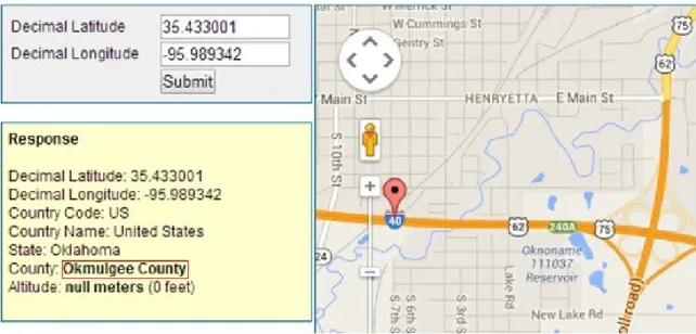
The county that a WIM station belongs to could be determined by GPS coordinates from website: http://labs.silverbiology.com/countylookup/. For example, WIM 6 belongs to Okmulgee County, and it belongs to Division 1 (shown in Figure 2.4).
16
Figure 2.4 Determining County of The Sample WIM Site Division and county information for all WIM sites is summarized in Table 2.3
Step 3: Obtaining Soil Data
Subgrade soil data, including AASHTO soil classification, sieve analysis, soil constants, and suitability, are obtained from ODOT's Geologic Materials Classification (Red Books) (24). Figure 2.5 shows an example on how to obtain soil data for WIM6
pavement site. The summary of soil information for all pavement sites is shown in Table 2.3, which is then used for subgrade input for MEPDG.
17
Table2.3 Division and County of WIM Sites
WIM Division County Geologic Unit Soil Classification Sieve 10 Sieve 40 Sieve 60 Sieve 200
1 8 Washington Chanute A6 100 86 82 65 2 3 Murray Alluvium A6 100 98 97 94 3 4 Oklahoma Hennessey A4 100 95 79 52 5 8 Mayes Hartshorne-Atoka A4 100 85 79 61 6 3 Okfuskee Wewoka A6 99 98 97 96 7 5 Blaine Alluvium A6 100 99 99 97
9 3 Pontotoc Francis A-7-6 100 99 99 98
10 2 Pittsburg Boggy A6 100 99 98 96
11 7 Grady Rush Spring A4 100 100 100 73
16 8 Mayes McAlester A-7-6 100 100 99 95
21 2 Bryan Terrace Deposits A-7-6 100 95 85 75
22 2 Le Flore McAlester A4 100 96 92 81
23 6 Major Terrace A4 100 95 85 75
27 4 Kay Wellington A-7-5 100 99 98 91
28 4 Canadian Blaine A4 100 100 97 73
29 1 Sequoyah McAlester A4 100 93 91 88
30 3 McClain Hennessey A6 99 98 97 96
104 4 Logan Garber A6 100 99 99 88
114 5 Washita Elk City A4 100 99 98 91
18
19 Step 4: Designing Pavement Thickness
The most commonly used Superpave mixture types in Oklahoma are S3 and S4 defined in the ODOT Standard Specification Book (22). Two inches of S3 mixture using PG76-28 asphalt binder is designed as the surface functional course. Beneath that, S4 mixture binder layer with PG70-22 binder is applied for all the sites. Since Level 1 testing data for hot-mix asphalt (HMA) and asphalt binder are not available, Level 3 inputs based on typical mixture gradation are used. Three base materials are commonly used in
Oklahoma: granular aggregate, lime treated, and fly ash treated. Pavement structures are designed following the 1993 AASHTO Guide using field collected AADTT with a growth rate of 4%. The designed layer thicknesses are summarized in Table 2.4.
Simulated Traffic Input Scenarios Data Sources
For the 23 WIM sites, the WIM traffic monitoring data are saved into four file types following the FHWA Traffic Monitoring Guide (TMG) formats (12): station description data, traffic volume data, vehicle classification data, and truck weight data. Raw WIM data in 2008 are obtained from Oklahoma Department of transportation (ODOT) and used in this paper. Three of the WIM sites (WIM 8, 25 and 32) don't have completed data sets and are excluded from analysis. The locations of the 20 WIM sites with complete coverage of a year data (from January to December) has already been demonstrated in Figure 2.2
20
Table2.4 1993 AASHTO Pavement Design Results
WIM
Site AADTT
AC Thickness (in.) Base Layer
Subgrade Surface Layer
(S3 Mix)
Binder Layer
(S4 Mix) Material Type
Thickness (in.)
1 1876 2 6 Granular Aggregate + Lime Treated 6 + 6 A-6
2 6907 2 9 Granular Aggregate 8 A-6
3 8496 2 9 15% Fly Ash Treated 7 A-4
5 4037 2 8 Granular Aggregate 6 A-4
6 5316 2 9 Granular Aggregate 6 A-6
7 1413 2 7 15% Fly Ash Treated 6 A-6
9 1260 2 8 Granular Aggregate 6 A-7-6
10 4880 2 9 15% Fly Ash Treated 6 A-6
11 1518 2 7 Granular Aggregate 6 A-4
16 3096 2 9 15% Fly Ash Treated 6 A-7-6
21 1316 2 6 Granular Aggregate + Lime Treated 6 + 7 A-7-6
22 1225 2 6 15% Fly Ash Treated 7 A-4
23 1039 2 4 Granular Aggregate + Lime Treated 6 + 8 A-4
27 4600 2 8 Granular Aggregate + Lime Treated 6 + 6 A-7-5
28 9523 2 9 Granular Aggregate 8 A-4
29 6721 2 9 15% Fly Ash Treated 6 A-4
30 10427 2 9 Granular Aggregate + Lime Treated 6 + 6 A-6
104 6263 2 8 Granular Aggregate + Lime Treated 6 + 6 A-6
114 8255 2 8 Granular Aggregate + Lime Treated 6 + 6 A-4
21
The raw WIM data are processed using the Prep-ME software (18), the final product of the Transportation Pooled-Fund study TPF-5(242): Traffic and Data Preparation for AASHTO Pavement-ME Analysis and Design. Particularly, Prep-ME is capable of pre-processing, importing, checking the quality of raw WIM traffic data, and generating three levels of traffic data inputs with in-built clustering analysis methods for MEPDG.
Traffic Input Scenarios
Twelve traffic scenarios within four groups are proposed to simulate different traffic level of inputs from various traffic data acquisition technologies and time coverage of the data collection. All this calculations are performed in the Prep-ME software.
Group #1: Site-Specific WIM Data with Various Time Coverage.
Scenario 1 - Continuous Site-Specific WIM Data. This scenario has high quality continuous 12-month of WIM data within a year, which represents the most complete traffic data sets required in the MEPDG, and it is defined as the "reference" traffic data.
Scenario 2 - Site-Specific WIM with 1 Month Data per Season. This scenario involves WIM data that cover 1 month in each of the four seasons, representing situations that only partial of the WIM data can pass WIM data quality check ("good data") while those cannot pass QC ("bad data") are replaced with "good data". In other words, the traffic volume by truck class is not known for all months of a year. The WIM data in January, April, July and October are selected to represent the four seasons for winter, spring, summer, and fall. The traffic
22
inputs for this scenario are simulated from the continuous WIM data sets in Scenario 1 for all the 20 WIM sites.
Scenario 3 - Site-Specific WIM with 1 Week Data per Season. This scenario simulates traffic data collected using portable WIM systems. One week of portable WIM data are collected in each season. Each week was assumed to be representative of the entire season. The traffic data inputs for this scenario are simulated from the continuous WIM data sets in Scenario 1. To exclude holidays, the data from 7th to 13th in January, April, July and October are used to represent winter, spring, summer, and fall.
Group #2: Site-Specific Classification Data with Various Time Coverage and Statewide WIM Load Data
Scenario 4 - Continuous Site-Specific Classification Data and Statewide WIM Load Data. This scenario used only the vehicle classification information that is available from the 20 WIM sites being analyzed. It represents the situation that only continuous site specific AVC data but no WIM load data is available. The average statewide axle loading data are used. This scenario is parallel to Scenario 1.
Scenario 5 - Site-Specific Classification with 1 Month Data per Season and Statewide WIM Load Data. This scenario is parallel to Scenario 2. This scenario involves only one month of classification data in each of the four seasons. It simulates the situation that AVC data in some months is either not collected or
23
has unacceptable data quality. Those data is replaced with other month’s good data.
Scenario 6 - Site-Specific Classification with 1 Week Data per Season and Statewide WIM Load Data. This scenario is parallel to Scenario 3. This scenario involves only one week of classification data in each of the four seasons. It
simulates the data collection technique using short-term classification counts.
Group # 3: Regional and National Defaults
Scenario 7 - Statewide vehicle classification and LTPP TPF-5(004) Defaults load spectra. The LTPP TPF-5(004) study: Long-Term Pavement Performance (LTPP) Specific Pavement Study (SPS) Traffic Data Collection (19) has
developed axle loading defaults based on the 26 LTPP pooled-fund study WIM sites. Three tiers of loading group are developed: Tier 1 for "Global" axle loading defaults, Tier 2 for "Typical" defaults, and Tier 3 for site-specific data. In this scenario, Tier 2 "Typical" axle loading defaults and State average vehicle classification.
Scenario 8 - State Averages. In this scenario, statewide averages of axle loading and truck volume adjustment factors are used.
Scenario 9 - National MEPDG Defaults. In this scenario, national MEPDG defaults are used. The default VCD factors are determined based on TTC classes from the MEPDG software.
24
Group #4: 48 Hour Short-Term Class Counts Using Various Clustering Methods In most practical cases, when pavements are designed, no prior Level 1 traffic WIM data are available and highway agencies opt not to use Level 3 inputs. Generally Levels 2 (clustering average) traffic inputs are considered for design by combining existing site-specific data from WIM systems located on sites that exhibit similar traffic
characteristics. How to qualify these similarities and how to develop loading groups for pavement design is a recent interest in the US. This group provides three example clustering methods, ranging from simple to complex, to investigate the impact of axle loading on pavement performance.
Scenario 10 - 48 Hour Short-Term Class Counts Using TTC Method. Recognizing that highways within the same functional classification have significant variability in truck distribution, MEPDG proposes the truck traffic classification (TTC) methodology for pavement structural design purposes to describe the distribution of trucks traveling on roadway (2). In this scenario, 48 hours of truck classification data on June 10th and June 11th are used to compute site specific VCD factors after monthly and DOW adjustment, and to determine the TTC class for each of the 20 design site. Traffic averages for each TTC class are obtained for MEPDG. This scenario simulates the situation that only short-term 48-hour truck counts data is available. A summary of 48-hour VCD and TTC Class for each WIM site is shown in Table 2.5.
25
Table2.5 48-hour VCD and TTC Class
WIM C4 C5 C6 C7 C8 C9 C10 C11 C12 C13 TTC Class 1 1.5 41.8 4.2 0.3 11.6 38.6 0.7 0.1 0.1 0.1 9 2 1.0 11.6 2.0 0.1 7.1 72.7 0.5 2.3 1.6 0.2 1 3 0.8 72.8 3.0 0.1 8.8 11.7 0.6 0.8 0.1 0.3 14 5 0.6 8.3 1.4 0.1 2.6 80.3 0.6 3.2 1.0 0.1 1 6 1.1 12.0 1.7 0.1 5.8 72.7 0.8 2.9 1.2 0.7 1 7 0.6 26.3 2.7 0.1 10.6 56.3 1.1 0.5 0.4 0.3 4 9 1.7 39.8 9.3 0.4 5.8 41.3 1.1 0.2 0.2 0.2 6 10 0.6 11.5 1.8 0.1 2.2 77.2 0.6 3.2 0.9 0.1 1 11 1.4 50.5 4.0 0.2 13.4 27.6 0.9 0.3 0.1 0.7 12 16 1.5 42.8 3.2 0.2 9.7 40.3 0.4 0.6 0.2 0.2 12 21 1.5 17.5 0.7 0.0 3.8 69.0 0.5 3.6 1.2 0.1 2 22 1.4 48.5 2.3 0.5 9.9 34.9 0.9 0.0 0.2 0.3 12 23 1.1 46.7 2.6 0.1 11.2 36.1 1.5 0.5 0.2 0.1 12 27 0.8 9.5 1.7 0.0 4.0 77.2 0.5 2.7 2.0 1.6 1 28 1.0 18.8 2.5 0.1 2.5 71.0 0.7 1.8 1.4 0.2 1 29 1.0 9.5 1.4 0.1 6.3 76.6 0.3 2.5 1.3 0.1 1 30 1.4 19.1 2.5 0.3 8.5 62.5 0.6 2.7 1.2 0.2 2 104 1.5 20.4 2.4 0.2 7.1 62.6 0.8 2.2 1.6 1.3 2 114 0.9 14.2 1.7 0.1 2.5 72.8 0.9 2.0 1.6 0.1 1 118 1.7 32.5 2.3 0.1 9.1 52.3 0.6 0.4 0.1 0.1 4 Scenario 11 - 48 Hour Short-Term Class Counts Using KYTC Method.
Kentucky Transportation Cabinet (KYTC) has proposed an aggregated class method based on highway functional class to prepare traffic data for pavement deign (20). The detailed aggregated classes are shown in Table 2.6. This scenario is similar to Scenario 10 but using KYTC method to obtain traffic average data for MEPDG.
26
Table2.6 Aggregation Class for Traffic Inputs in Kentucky Transportation Cabinet (KYTC)
Aggregate
Class Functional Class
Class I Rural Interstate (FC1)
Class II Rural Principal Arterial (FC2) Rural Minor Arterial (FC6)
Class III
Rural Major Collector (FC7) Rural Minor Collector (FC8) Rural Local (FC9)
Class IV Urban Interstate (FC11)
Class V
Urban Other Freeway and Expressway (FC12)
Urban Other Principal Arterial (FC14)
Class VI
Urban Minor Arterial (FC16) Urban Collector (FC17) Urban Local (FC19)
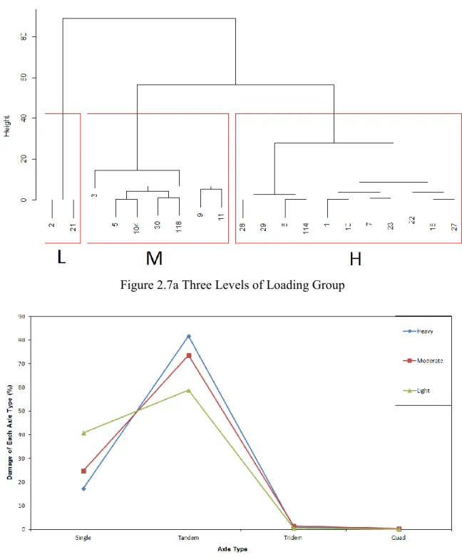
Scenario 12 - 48 Hour Short-Term Class Counts Using Loading Group Method. In this scenario, loading groups are developed based on the North Carolina DOT clustering method, which is provided in the Appendix G of the 2013 version of Traffic Monitoring Guide (21). Damage factor metric is developed by NCDOT to investigate the fatigue damage caused by a particular axle type within a particular weight load bin. It is found that more than 99% of total damage is caused by Single and Tandem axle types, and therefore Tridem and Quad axle types can be excluded from the loading group development (21). Following the NCDOT procedure, the damage factors for each of the 20 WIM
27
sites are developed for each WIM station. It found that WIM data from Oklahoma DOT shows a similar character to NCDOT: about 99% of damage comes from Single and Tandem axles (shown in Table 2.7).
Table2.7 Damage Caused By Each Axle Type WIM Single Tandem Tridem Quad
1 19.74 79.36 0.83 0.08 2 40.69 58.84 0.42 0.05 3 29.76 66.88 2.74 0.62 5 22.82 76.80 0.35 0.03 6 13.71 83.71 0.54 0.05 7 20.12 77.46 2.24 0.18 9 26.69 71.92 1.27 0.12 10 20.02 79.31 0.60 0.07 11 22.24 72.45 2.46 0.85 16 18.29 81.00 0.66 0.06 21 40.86 58.70 0.40 0.04 22 16.01 81.45 2.22 0.31 23 19.78 78.12 1.94 0.15 27 18.33 81.31 0.35 0.01 28 13.99 85.65 0.31 0.04 29 14.08 85.60 0.30 0.02 30 23.72 73.34 0.76 0.17 104 22.55 76.65 0.70 0.10 114 14.95 83.39 0.61 0.05 118 23.13 74.28 0.55 0.05 Average 22.22 76.56 1.06 0.15
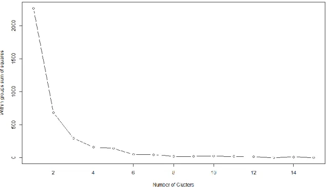
Subsequently, hierarchical clustering analysis is applied to the damage spectra of four axle types. Clustering analysis including determining the number of clusters is achieved with the open source software R. Number of clusters is the first factor
28
that is decided in this study. Figure 2.6 is generated by R and is used to determine number of clusters in this research. The horizontal axis means number of clusters and the vertical axis means sum of variance within each group. An optimized number of clusters should balance these two numbers. According to this rule, three loading groups are identified with distinctive levels of load patterns (Light, Moderate, and Heavy) as shown in Figure 2.7a and Figure 2.7b. More information about clustering analysis can be found in the work by Wang et al. (25). Average traffic inputs of the load groups are obtained for each of the 20 WIM sites.
29
Figure 2.7a Three Levels of Loading Group
30 Other Inputs for MEPDG
AADTT & Traffic Growth Rate
AADTT and traffic growth rate are the basic inputs for MEPDG. The field AADTT values are obtained from the 2009 Oklahoma Traffic Characteristics Report (23). In order to examine the impact of AADTT variations on pavement performance, three AADTT levels are studied for each site: low (0.5 times of field AADTT), normal (field AADTT), and high (1.5 times of field AADTT). Two growth rates are included: 2% for the lower level and 4% for the higher level
Operating Speed
All the WIM sites are located on National Highway Systems (NHS). The typical highway speed is from 60 mph to 75mph. In this study, 70 mph is applied to all WIM sites.
Axle per Truck
In this study, statewide "Number of Axles per Truck" values rather than MEPDG default are used for all designs (except for Scenario 9, MEPDG default), the most significant difference between these two groups of inputs is that Statewide values take quad axles into consideration, so it shall be more accurate than the MEPDG default in this research. The comparison of these two data sets is shown in Table 2.8.
Climate
Climate data are generated by the MEPDG software based on the WIM site GPS coordinates. Altitude data is acquired from the website
http://www.daftlogic.com/sandbox-google-maps-find-altitude.htm from the GPS
coordinates. A typical value of 10 feet of ground water level is applied for all WIM sites. A summary of altitude for all WIM sites is shown in Table 2.9.
31
Table2.8Statewide and MEPDG Default “Axles per Truck”
Statewide MEPDG Default
Single Tandem Tridem Quad Single Tandem Tridem Quad
Class 4 1.49 0.5 0 0 1.62 0.39 0 0 Class 5 1.89 0 0 0 2 0 0 0 Class 6 1 1 0 0 1.02 0.99 0 0 Class 7 1.22 0.22 0.61 0.13 1 0.26 0.83 0 Class 8 2.21 0.76 0 0 2.38 0.67 0 0 Class 9 1.29 1.85 0 0 1.13 1.93 0 0 Class 10 1 1 0.95 0.02 1.19 1.09 0.89 0 Class 11 3.8 0.02 0.05 0 3.29 0.26 0.06 0 Class 12 2.85 1.01 0.04 0.01 2.52 1.14 0.06 0 Class 13 2.25 1.18 0.35 0.16 2.25 2.23 0.35 0
Table2.9Altitude of WIM Sites In Oklahoma WIM ID Altitude (ft) 1 700.708 2 795.041 3 1263.125 5 592.439 6 782.654 7 1500.295 9 960.126 10 626.902 11 1330.407 16 642.043 21 630.176 22 430.013 23 1322.493 27 1005.426 28 1320.431 29 521.346 30 1158.428 104 1124.408 114 1918.004 118 1280.191
32 Percent of Truck In Design Lane
Lane distribution factor, the percentages of trucks on the design lane, is another traffic factor. For pavement sections that have two lanes in one direction, a typical number of 95% is applied, while for the two pavement sections where WIM 22 and WIM 23 locates, there is only one lane in each direction and 100% is used for the lane distribution factor.
Percent of Truck In Design Direction
Since no site-specific direction factor information is available, 50% is applied for all design and analysis, which means that traffic of the two different direction is equal.
33 CHAPTER III
MEPDG RESULTS ANALYSIS
MEPDG Pavement Performance
Considering 20 pavement sites, 12 simulated traffic data collection scenarios, 3 AADTT level, and 2 growth rates, 1,440 MEPDG runs are performed. For each run, the following MEPDG pavement performance data are predicted:
Fatigue cracking (bottom-up alligator) in percentage (%), Longitudinal cracking (top-down longitudinal) in ft/mi., Total plastic deformation in terms of total rutting in inches,
Roughness in terms of international roughness index (IRI) in in/mi.
Impact of Traffic Level
Three traffic levels are defined to examine the impacts of traffic level on pavement performance:
Low: 0.5 times of field AADTT with 2.0% growth rate, Medium: field AADTT with 4% growth rate,
High: 1.5 times of field AADTT with 4% growth rate.
34
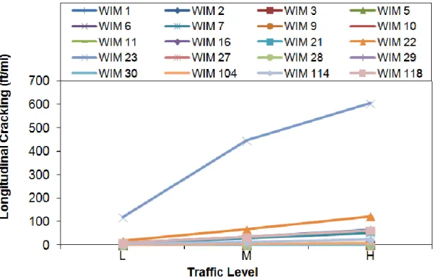
Figure 3.1a Pavement Performance (Long. Crack) at Various Traffic Levels
35
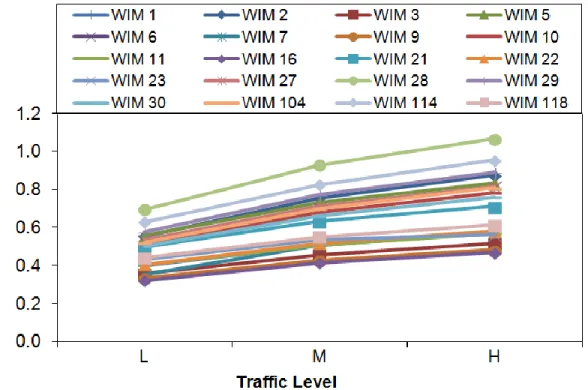
Figure 3.1c Pavement Performance (Rutting) at Various Traffic Levels
36
At the end of the 20-year design life, the predicted fatigue cracking is less than 2% for all the 20 sites. All sites except the pavement sections located at WIM22 and WIM23 are predicted to have less than 100 ft/mi of longitudinal cracking. The predicted longitudinal cracking values at WIM22 section are 17.6 ft/mi, 66.9 ft/mi, and 123 ft/mi for low, medium, and high traffic levels, while those at WIM23 section are 120 ft/mi, 448 ft/mi, and 605 ft/mi. This may because that WIM 23 has only 4 inches of binder layer, roughly 2/3 to half of other sites. The default recommended design limits in the MEPDG software for arterial roads are 25% for fatigue cracking and 2000 ft/mi for longitudinal cracking. Therefore, it is concluded that all the 20 sites don't show potential failure in terms of longitudinal cracking and fatigue cracking.
The default recommended design limits in MEPDG are 0.75 inches for total pavement rutting and 172 in/mi for terminal IRI. As can be seen in Figure 3.1, many sites will fail at the end of 20-year design life according to these two criteria. For example, at WIM28 section, the predicted total rutting at the end of 20-year, are 0.695 inches, 0.928 inches, and 1.068 inches, while the predicted IRI are 163.02 in/mi, 174.22 in/mi, and 182.57 in/mi.
The difference of predicted pavement performance for the three traffic levels is shown in Figure 3.2a, b, c and d. The predicted differences of longitudinal cracking and fatigue cracking are significant.
37
Figure 3.2a Pavement Performance Changes (Long. Crack) at Various Traffic Levels
38
Figure 3.2c Pavement Performance Changes (Rutting) at Various Traffic Levels
39
If comparing to the "Medium" traffic level, only 25% of longitudinal cracking and 38% of fatigue cracking are predicted for low traffic level, while 181% of longitudinal cracking and 150% of fatigue cracking for high traffic level. There are on average more than 20% differences of rutting predictions. The average predicted total rutting for the three travel levels are 0.47 inches, 0.62 inches, and 0.72 inches. For predicted IRI, the average difference is 5%, which is approximately 7.5 in/mi of IRI difference.
Impact of WIM Data Coverage
The predicted pavement performance and the differences for Scenarios 1, 2 and 3 are plotted in Figure 3.3a, b, c and d. Since very few fatigue cracks are predicted and longitudinal cracking shows no potential failure, only IRI data and total rutting data are presented. Scenario 1 with continuous site-specific WIM data is used as the reference scenario. Even though variations are observed for the predicted longitudinal cracking and total rutting for the 20 pavement sites, the differences among these three scenarios are generally small. Comparing to Scenario 1, Scenario 2 and Scenario 3 predicts -3.65 to 1.01 inch/mile of IRI, and 100.01% and 99.68% of total rutting.
Therefore, it can be concluded that the traffic data from the three scenarios with various WIM data coverage results in minor difference of pavement performance. Collecting short-term one week WIM data per each season is adequate to provide accurate traffic classification and loading data for MEPDG.
40
Figure 3.3a Predicted Pavement Performance Changes (IRI) with Various WIM Data Coverage (Scenarios 1, 2, 3)
Figure 3.3b Predicted Pavement Performance Changes (Rutting) with Various WIM Data Coverage (Scenarios 1, 2, 3)
41
Figure 3.3c Predicted Pavement Performance (IRI) with Various WIM Data Coverage (Scenarios 1, 2, 3)
Figure 3.3d Predicted Pavement Performance (Rutting) with Various WIM Data Coverage (Scenarios 1, 2, 3)
42 Impact of Vehicle Distribution
The predicted pavement performance and the differences for Scenarios 4, 5 and 6 are plotted in Figure 3.4a, b, c and d. Comparing to the reference Scenario 1, Scenarios 4, 5, and 6 predict -4.46 to 6.21 inch/mile of IRI, and 104.2%, 104.2%, 105.6% of total rutting. Two observations can be made based on the comparisons:
The three scenarios using site-specific truck classification data but with different time coverage generate comparable pavement performance prediction. In other words, collecting one week short-term truck classification data per each season is adequate to provide accurate traffic classification data for MEPDG. In order to obtain annual or monthly average traffic volume for each truck class to calculate VCD and monthly adjustment factors (MAF), the short-term weekly data should be adjusted by day of week for each month to remove biases using existing long-term traffic data. The accuracy of VCD and MAF generation is depending on the quality of the existing long-term data within a highway agency. Due to the fact that Scenarios 4, 5, 6 use statewide axle load data rather than site-specific WIM data, these three scenarios predict higher longitudinal cracking and total rutting, which indicates that axle loading data have impacts on
43
Figure 3.4a Predicted Pavement Performance Changes (IRI) with Various Classification Data Coverage (Scenarios 4, 5, 6)
Figure 3.4b Predicted Pavement Performance Changes (Rutting) with Various Classification Data Coverage (Scenarios 4, 5, 6)
44
Figure 3.4c Predicted Pavement Performance (IRI) with Various Classification Data Coverage (Scenarios 4, 5, 6)
Figure 3.4d Predicted Pavement Performance Changes (Rutting) with Various Classification Data Coverage (Scenarios 4, 5, 6)
45 Use of Regional and National Defaults
Results for Scenarios 7, 8 and 9 are plotted in Figure 3.5a, b, c and d. The predicted pavement performance demonstrates very consistent results. Comparing to reference Scenario 1 with Level 1 WIM input, Scenario 8 (Statewide traffic averages) generates the most accurate results, followed by Scenario 7 (the LTPP-5(004) typical defaults), and Scenario 9 (MEPDG defaults). In all cases, Scenario 8 outperforms Scenario 9 by a wide margin with much accurate predictions. On average, Scenarios 7, 8 and 9 predict -5.93 to 21.36 inch/mile of IRI, and 118.8%, 107.2%, 131.4% of total rutting. Using MEPDG default may cause significant errors of performance prediction. At minimum highway agency should use statewide average for the implementation of MEPDG if site-specific WIM data are not available. The LTPP pooled-fund study TPF-5(004) Tier 2 "Typical" defaults generate better results than those based on MEPDG defaults. However,
significant differences of the predicted performance are observed at several sites. Since LTPP TPF-5(004) defaults were developed based on only 26 LTPP WIM stations, the traffic results may not be applicable for some highway agencies to use them as traffic inputs.
46
Figure 3.5a Predicted Pavement Performance Changes (IRI) with Regional/National Traffic Defaults (Scenarios 7, 8, 9)
Figure 3.5b Predicted Pavement Performance Changes (Rutting) with Regional/National Traffic Defaults (Scenarios 7, 8, 9)
47
Figure 3.5c Predicted Pavement Performance (IRI) with Regional/National Traffic Defaults (Scenarios 7, 8, 9)
Figure 3.5d Predicted Pavement Performance (Rutting) with Regional/National Traffic Defaults (Scenarios 7, 8, 9)
48 Impact of Axle Loading
The predicted pavement performance and the differences for Scenarios 10, 11 and 12 are plotted in Figure 3.6a, b, c and d. On average, scenarios 10, 11, and 12 predict -8.48 to 10.8 inch/mile of IRI, and 99.7%, 103.6%, 101.6% of total rutting. Comparing to Scenarios 7, 8, 9 using regional of national averages for axle loading, Scenarios 10, 11, 12 using clustering approaches generate more accurate results, which indicates that developing load groups is necessary to prepare better traffic data for the implementation of MEPDG.
Theoretically, Scenarios 10, 11, 12 should generate more accurate pavement performance prediction results than those from Scenarios 4, 5, 6. However, comparing to Scenarios 4, 5, 6 using site-specific classification data and statewide axle loading, these three
scenarios based on 48-hour classification counts and clustering approaches produce comparable pavement performance predictions. This may be due to two reasons. Firstly, Scenario 10, 11, 12 use 48-hour classification data to predict AADTT for each truck class may not be as accurate as those predicted from continuous, one month per season, and one week per season classification data. As a result, the pavement performance prediction accuracy is sacrificed. Secondly, it may indicate that the three clustering approaches are not the optimized algorithms to group Oklahoma traffic patterns. The TTC approach (Scenario 10) only takes truck classification data but not weight data into consideration; the KYTC method (Scenario 11) is fundamentally based on highway functional class and may not be adequate to characterize truck patterns; the loading group method (Scenario 12) depends on the clustering results from North Caronia DOT. Therefore it is suggested
49
developing state specific truck traffic patterns in order to generate accurate traffic load spectra for MEPDG.
Figure 3.6a Predicted Pavement Performance Changes (IRI) with Various Axle Loading Methods (Scenarios 10, 11, 12)
50
Figure 3.6b Predicted Pavement Performance Changes (Rutting) with Various Axle Loading Methods (Scenarios 10, 11, 12)
Figure 3.6c Predicted Pavement Performance (IRI) with Various Axle Loading Methods (Scenarios 10, 11, 12)
51
Figure 3.6d Predicted Pavement Performance (Rutting) with Various Axle Loading Methods (Scenarios 10, 11, 12)
52 CHAPTER IV
DISCUSSIONS
One pair of WIM sites with comparable AADTT and pavement structures are selected to provide detailed comparisons of traffic inputs from the 12 simulated scenarios: WIM 2 on I-35 2.6 miles south of Jt. SH-7 with an AADTT of 6907 and WIM 29 on I-40 0.5 Miles East Mile Marker 311 with an AADTT of 6721. Both sites are classified as highway functional class 1 (Rural Major Collector). Based on the loading group results from Scenario 12, WIM 2 belongs to "Light" axle loading group, while WIM 29 belongs to "Heavy" axle loading group.
The vehicle class distributions of these two sites are shown in Figure 4.1a and b. All simulated scenarios except for Scenario 8 (State Averages) generate very similar results. Dominant percentage of class 9 long-haul vehicles are observed on the two sites. The MEPDG VCD defaults (Scenario 9) are the national averages for the general roadway category of "Principal Arterials - Interstates and Defense Routes". Because the state averages consider both long-haul interstates and local short-haul truck routes (generally with higher percentage of class 5 trucks), Scenario 8 demonstrates much higher
53
Figure 4.1a VCD For WIM 2
54
For All other scenarios, including those use site-specific one month or one week truck data per season, and 48-hour truck count data, develop almost identical VCD inputs. Therefore, at minimum 48-hour site-specific truck class count data rather than using state or national averages are required to obtain accurate VCD inputs.
The tandem axle load distributions are summarized in Figure 4.2a and b. Scenarios 1, 2, and 3 produce almost identical axle loading data with two peaks, representing empty or lightly-loaded versus full-loaded heavy axles. WIM 2 has approximately equal
percentage of empty and fully- loaded peaks, while WIM 29 has much higher percentage of fully-loaded axles and less empty axles. The peaks for WIM 2 are located at 10kips and 26kips, while WIM 29 carries heavier loads with two peaks at 12kips and 30kips. For WIM 2 site, axle loading spectra for Scenarios 10, 11, and Scenarios 4, 5, 6, 8 using state averages demonstrate similar trends, but have lower percentage of axle load bins at the two peaks, and higher parentages of heavy load bins greater than 30kips. For WIM 29 sites, Scenarios 4, 5, 6, 8, 10, 11 have comparable peak 1 and heavy load bins greater than 30kips, but lower percentage of axle load bins at the second peak. Scenarios 7 and 9 in Group 3 predict significant different tandem axle loading. Scenario 7 based on LTPP method shows abnormally high percentages of light axles around 6kips and 8kips, while Scenario 9 using national defaults demonstrates much higher percentages of heavy loads greater than 34kips. In addition, Scenario 12 also develops different load patterns for WIM 29 site with heavier second peak located at 30kips.
55
Figure 4.2a Tandem Axle Loading for WIM 2
56
The monthly adjustment factors for vehicle class 5 and class 9 are illustrated in Figure 4.3a, b, c and d. Class 5 trucks on both sites show significant variations of monthly truck volume, while the volume for class 9 is relatively consistent within all scenarios.
Scenarios with either site-specific WIM data or site-specific classification data (Scenarios 2, 3, 4, 5, 6) can establish as accurate MAFs as those from the reference Scenario 1. Scenario 9 using national defaults and Scenario 10 based on TTC method demonstrate minor monthly variations. Scenario 8 based on state averages, Scenario 11 based on KYTC method, and Scenario 12 based on loading group method show notable
differences of monthly factors. It should be noted that there is significant drop of class 9 trucks in November and December, probably due to the holidays.
The above discussions also indicate that no two sites share the same traffic
characteristics. Truck volumes and weights can vary considerably from road to road and even from location to location along a road. Therefore, using site-specific data when possible is recommended for MEPDG. Short-term site-specific data if appropriately adjusted to annual average data can generate accuracy traffic inputs.
57
Figure 4.3a MAF (Class 5 Vehicle) for WIM 2
58
Figure 4.3c MAF (Class 9 Vehicle) for WIM 2
59 CHAPTER V
CONCLUSIONS
Recognizing that many highway agencies do not have the resources to collect continuous Level 1 WIM traffic data to accurately characterize future traffic for MEPDG, this study investigates the variability and impacts of traffic data on MEPDG predicted performance. Twelve traffic data input scenarios are simulated to include a combination of various traffic data acquisition technologies and length of time coverage at 20 WIM sites in Oklahoma. In total 1,440 MEPDG runs are performed for 3 AADTT levels and 2 growth rates. Based on comparison analyses, the following conclusions are made to guide highway agencies to prepare traffic data for the implementation of MEPDG:
Base year AADTT and traffic growth rate have significant impact on pavement performance.
Using traffic data from site-specific WIM sites with various lengths of time coverage results in minor difference of pavement performance. Collecting one week short-term WIM data per each season is adequate to provide accurate traffic classification and loading data for MEPDG.
60
Truck volumes and weights can vary considerably from road to road and even from location to location along a road. Using site-specific data, either short-term or long-term, when possible is recommended.
If properly adjusted short-term data by day of week for each month, collecting one week classification data per season is adequate to provide truck adjustment data. At minimum 48-hour site-specific truck class count data are recommended to obtain VCD inputs.
Axle loading data have impacts on pavement performance. Developing state specific truck traffic patterns is recommended to generate traffic load spectra. Using regional or national default inputs, especially MEPDG defaults, may cause
significant errors of performance prediction. At minimum highway agency should use statewide average if site-specific WIM data are not available.
61
REFERENCES
1. American Association of State Highway and Transportation Officials (AASHTO). Guide for the Design of Pavement Structures. Washington, D.C. American
Association of State Highway and Transportation Officials, 1993.
2. NCHRP 1-37A. Guide for Mechanistic-Empirical Design of New and Rehabilitated Pavement Structures. Applied Research Associates Inc. ERES Consultants Division, Urbana Champion, IL, 2004.
3. Schwartz Charles W. and Rui Li. Sensitivity Evaluation of MEPDG Performance Prediction, NCHRP Research Results Digest, Issue 372, 2013.
4. Cooper, Samuel B., Elseifi, Mostafa A. and Mohammad, Louay N. Parametric Evaluation of Design Input Parameters on the Mechanistic-Empirical Pavement Design Guide Predicted Performance. International Journal of Pavement Research and Technology, Vol. 5, Issue 4, 2012, pp. 218-224.
62
5. Li Jianhua., Linda M. Pierce, Mark E. Hallenbeck, and Uhlmeyer, Jeffrey S. Sensitivity of Axle Load Spectra in the Mechanistic-Empirical Pavement Design Guide for Washington State. Journal of the Transportation Research Board, Issue 2093, 2009, pp. 50-56.
6. KhanumTaslima, Mustaque Hossain, Stefan A. Romanoschi and Richard Barezinsky. Concrete Pavement Design in Kansas Following the Mechanistic- Empirical
Pavement Design Guide. Proceedings of the 2005 Mid-Continent Transportation Research Symposium, Ames, Iowa, 2005.
7. KhanumTaslima., Mustaque Hossain, and Greg Schieber. Influence of Traffic Inputs on Rigid Pavement Design Analysis Using Mechanistic-Empirical Pavement Design Guide. Annual Meeting of Transportation Research Board. CD-ROM. National Research Council, Washington, DC, 2006.
8. Sauber Robert W., Nicholas P. Vitillo, Sameh. Zaghloul, Amr Ayed, and Amir Abd El Halim. Sensitivity Analysis of Input Traffic Levels on Mechanistic-Empirical Design Guide Predictions. Annual Meeting of Transportation Research Board. CD-ROM. National Research Council, Washington, DC, 2006.
9. Tran, Nam H., and Kevin D. Hall. Development and Influence of Statewide Axle Load Spectra on Flexible Pavement Performance. Journal of the Transportation Research Board, Issue 2037, 2007, pp. 106-114.
10. Sayyady, F., J. R. Stone, K. L. Taylor, F. M. Jadoun, and Y. R. Kim. Clustering Analysis to Characterize Mechanistic–Empirical Pavement Design Guide Traffic Data in North Carolina". Transportation Research Record 2160, Transportation Research Board, National Research Council, Washington, D.C., 2010, pp. 118-127.
63
11. Ritchie, S.G., and M.E. Hallenbeck, State-Wide Highway Data Rationalization Study, Research Report No. WA-RD-82.2, Washington State Department of Transportation, Olympia, WA, 1986.
12. Federal Highway Administration (FHWA). Traffic Monitoring Guide, 3rd edition. McLean, VA, 2001.
13. Papagiannakis A.T., M. Bracher, J. Li, and N. Jackson. Optimization of Traffic Data Collection for Specific Pavement Design Applications. Federal Highway
Administration (FHWA), McLean, VA, 2006.
14. Olga Selezneva, Ramachandran Aditya, Mustafa Endri, Carvalho Regis. Impact of Various Trucks on Pavement Design and Analysis: Mechanistic–Empirical Pavement Design Guide Sensitivity Study with Truck Weight Data. Journal of the
Transportation Research Board, Issue 2339, 2013, pp. 120-127.
15. Ala R Abbas, Frankhouser Andrew. Improved Characterization of Truck Traffic Volumes and Axle Loads for Mechanistic-Empirical Pavement Design. Ohio Department of Transportation Office of Research and Development and the U. S. Department of Transportation Federal Highway Administration, State Job Number 134557, 2012.
16. Jennifer K McCracken, Vandenbossche Julie M, Asbahan Rania E. Effect of the MEPDG Hierarchal Levels on the Predicted Performance of a Jointed Plain Concrete Pavement. 9th International Conference on Concrete Pavements. International Society for Concrete Pavements; Federal Highway Administration (FHWA);
64
17. Wang Kelvin C.P., Qiang Joshua Li, Stephen A. Cross, and Jeff Dean. MEPDG Distress Modeling for Oklahoma. The 2014 ASCE T&DI Congress, Orlando FL, 2013.
18. Wang Kelvin, Joshua Q. Li, Vu Nguyen, Mike Moravec, Doc Zhang. Prep-ME: An Multi-Agency Effort to Prepare Data for DARWin-ME. 2013 Airfield and Highway Pavements Conference, Los Angeles, CA, 2013.
19. Selezneva O.I. and M. Hallenbeck. Long-Term Pavement Performance Pavement Loading User Guide (LTPP PLUG). Applied Research Associates, Inc, Elkridge, MD, 2013.
20. Li Qiang Joshua, Kelvin C.P. Wang, and Zhongjie “Doc” Zhang. Traffic Loading Spectra Characterization for MEPDG in A Production Environment. The 2014 ASCE T&DI Congress, Orlando FL, 2013.
21. Federal Highway Administration (FHWA). Traffic Monitoring Guide, 4th edition. McLean, VA, 2013.
22. Oklahoma DOT (ODOT). Standard Specification for Highway Construction. Oklahoma City, Oklahoma, 2009
23. Oklahoma DOT (ODOT). 2009 Oklahoma Traffic Characteristics Report. Oklahoma City, Oklahoma, 2009.
24. Oklahoma Highway Department (OHD). Engineering Classification of Geologic Materials (Red Books). Oklahoma Research Project 61-01-1, Research and Development Division. Oklahoma City, Oklahoma, 1965.
65
25. Wang, K., Li, Q., Hall, K., Nguyen, V., and Xiao, D. Development of Truck Loading Groups for the Mechanistic-Empirical Pavement Design Guide. Journal of
Transportation Engineering, Vol. 137, Issue 12, 2011, pp. 855–862. 26. Kon
VITA JUNXIANG LOU Candidate for the Degree of
Master of Science
Thesis: EVALUATION OF TRAFFIC INPUT LEVELS FOR PAVEMENT ME DESIGN
Major Field: Civil Engineering Biographical:
Education:
Completed the requirements for the Master of Science in Civil Engineering at Oklahoma State University, Stillwater, Oklahoma in December, 2014.
Completed the requirements for the Bachelor of Science in Civil Engineering at Southwest Jiaotong University, Chengdu, Sichuan in China in 2012.
Experience:
Worked as an intern in China Southwest Research Institute of China Railway Engineering Company Limited in 2012
Worked for Kelvin Wang in Oklahoma State University in 2013 and 2014 Professional Memberships: ACI (American Concrete Institute)