Data Lineage and Meta Data Analysis in Data Warehouse Environments

(1)

Department of Informatics, University of Zürich

BSc Thesis

Data Lineage and Meta Data Analysis

in Data Warehouse Environments

Martin Noack

Matrikelnummer: 09-222-232 Email:[email protected]

January 31, 2013

(2)

Abstract

This thesis aims to provide new insights ondata lineagecomputations within the Credit Su-isse data warehouse environment. We propose a system to compute the lineage, targeted at business users without technical knowledge about IT systems. Therefore we provide complete abstraction for end users. Furthermore, we process only conceptualmapping rules from the metadata warehouse, in contrast to other approaches which record transformations at runtime, and consequently do not rely on access to potentially sensitive data. In order to process map-ping rules, we developed an algorithm that is capable of extracting components generically, based on their semantic meaning and relation to each other. This thesis describes some pat-terns in lineage investigations that result from our approach and gives an outlook to future projects that could be based on this work.

(3)

Zusammenfassung

Diese Arbeit erläutert unsere Erkenntnisse bezüglich der Berechnung von Data Lineage im Bereich des Data Warehouse der Credit Suisse. Hierzu stellen wir eine Methode vor, um Data Lineage für Business Anwender zu errechnen, welche keine tieferen Kenntnisse bezüglich der IT Systeme besitzen. Dem Benutzer wird mittels des vorgestellten Ansatzes vollständige Transparenz und Abstraktion vom technischen Problem ermöglicht. Wir benutzen lediglich die konzeptionellen Abbildungsvorschriften inMappingsaus dem Metadata Warehouse, wohinge-gen andere Ansätze die Abbildunwohinge-gen zur Laufzeit aufzeichnen. Daher sind wir nicht auf den Zugriff auf potentiell vertrauliche Daten angewiesen.

Um die Mapping Regeln auszuwerten, benutzen wir einen Algorithmus, der generisch ponenten aus Mappings ausliest. Dabei werden sowohl die semantische Bedeutung der Kom-ponenten, als auch deren Beziehung zueinander berücksichtigt. Weiterhin beschreiben wir in dieser Arbeit Muster in der Lineage Berechnung, die sich aus unserem Ansatz ergeben, und bieten ein Ausblick auf zukünftige Projekte basierend auf unseren Erkenntnissen.

(4)

List of Figures

3.1. Potential benefits of active lineage illustrated . . . 13

3.2. Example database for provenance considerations . . . 15

5.1. Real world example of a mapping . . . 20

5.2. Simplified form of the conceptual data model for mappings . . . 21

5.3. Excerpt from the used grammar . . . 21

5.4. Simple example mapping . . . 24

5.5. Parse tree built from a simple mapping . . . 24

6.1. Example for meta tree construction . . . 29

6.2. Part of the meta tree built from the grammar rules . . . 30

6.3. Simple example mapping . . . 33

6.4. Visualization of nodes and mappings . . . 38

7.1. Mappings with different structures . . . 43

7.2. Lineage on records . . . 44

(7)

List of Tables

6.1. Parameterized Nodes . . . 31

6.2. Result of the example query . . . 33

6.3. Result from the data selection . . . 33

6.4. Mapping components in a population . . . 37

(8)

1. Introduction

One of the core competencies of a a bank is the ability to maintain and efficiently utilize a data processing infrastructure [Lle96]. Especially analyzing large data sets to make market-based decisions or create a risk assessment for certain events provides valuable advantages [NB04]. As a middle-ware layer between transactional application and those decision supporting appli-cations, data warehouse systems are the technology of choice [Win01]. They serve as means to decouple systems used for the support of decision making from the business transactions. But by using those systems, data from different sources is quickly mixed and merged. In sev-eral steps complex computations are performed and results re-used in other steps. That makes it hard to keep track of distinct sources and influences during the numerous transformations that are necessary to compute the final result [EPV10], even though knowing the derivation history of data can be quite useful in many cases. For instance finding out about the trust-level attributed to certain sources and then assessing the reliability of the result is often very important [MM12]. Moreover, providing an audit-trail is common practice in many financial applications and has to be kept in great detail. In the simplest case, the user might just want to see and understand how exactly the result was created and which data items were used in the process.

The information about history and origins of data is called data provenance, or also data lin-eage [BKWC01]. In this thesis, we will address the issue of computing and analyzing the data lineage in data warehouse environments. In contrast to other approaches, we will not trace executed transformations, but use the conceptual logic behind single transformation rules to compute the flow of data independent from the technical implementation. This enables us to follow the lineage of data across various systems and implementations.

The transformation rules that we use are therefore not concrete implementations, such as SQL statements, but conceptual specifications of rules. They define on a conceptual level how data is transformed and moved along the system. Those rules are stored within the existing Credit Suisse metadata warehouse and calledmappings[JBM+_{12]. By following a sequence}

of mappings in reverse order, we can therefore find every source that may contribute to a given result according to the utilized sources in each mapping. In some cases, a sequence of mappings completely excludes data items from one or more sources by applying exclusive filters in different mappings. To recognize those restrictions, we process the conditional logic that is incorporated in every mapping and evaluate the combined conditions of the mapping sequence.

Consequently we propose a system to search for the source which contains the original data where a given result is effectively based on. We call this the golden source and the com-putation processactive lineage. However, the provided approach allows for many possible extensions in different directions, such as impact analysis or optimization of mappings.

(9)

The structure of this thesis is as follows: we will first describe the practical use case for our application in section 2. Then we define the scope of the thesis and describe the concrete task in chapter 3. To give the reader an idea of alternative solutions an how our approach compares to those, we will present the most common concepts in section 4. After presenting the existing elements on which we base our work in section 5, we will then explain the lineage computation in our system in section 6 and describe the developed algorithm in great detail. That is followed by an outline of common patterns that emerge from the proposed technique and what conclusions we can draw from them. Chapter 8 illustrates how the devised prototype implements the presented algorithm. In the last chapter 9 we will then give an outlook on future extensions of the algorithm based on its current limitations.

(10)

2. Use Case Description

As explained in chapter 1, lineage information describes the origins and the history of data. That information can be used in many scientific and industrial environments. A well docu-mented example of the importance of lineage information are tasks using SQL queries [MM12]. Here, the users often wants to find out why a particular row is part of the result or why it is missing. Those questions can usually be answered without much effort, since the user has direct access to and knowledge about the used queries.

While we will focus on a business related application, the usage of data lineage is of course not limited to those. Scientists in several fields such as biology, chemistry or physics often work with so-called curated databases to store data [BCTV08]. In those databases, data is heavily cross-connected and results originate from a sequence of transformations, not dissimilar to our application. Here it is vital for researchers to obtain knowledge about the origin of data. Depending on the source, they can then find the original, pure datasets and get a picture of their reliability and quality.

In the scope of this thesis, we primarily consider the internal processes in an internationally operating bank. Here exist many data sources that are part of different business divisions, such as Private Banking or Investment Banking. All of them serve different purposes and are maintained from different organizational units. Now, to create a reliable analysis or report as a basis for important decisions on a global scale, a system to support this has to take into account data from a potentially very large number of sources. In order to provide the expected result, data items may undergo a sequence of transformations over several layers in the system and are mixed or recombined [JBM+_{12]. We call such a transformation} _mapping_{, where a}

sequence of mappings defines a data flow, i.e. the path that data items take in the system, from their respective source to the final result. The full concept of those mappings and the implications will be explained in chapter 5.1. When the responsible user finally gets access to the report, there is practically no way for the human reader to grasp the complete data flow and its implications on single data items. Usually that would not be necessary for a business user who is only the initiator of the process and receiver of the result. But what if the user discovers a discrepancy in the generated data values? She might be able to verify the result or identify a possible error if she was presented with the details, since she is familiar with the purpose and operational origin of the data. Yet she can not be expected to have knowledge about the system on a technical level, especially not about the physical implementation of mappings. We therefore aim to provide a system that enables the user to gather lineage information about a given data item independent from her technical skills and knowledge. In order to built such a system, there are a number of issues to be addressed.

For example not every user has access to every part of the system. Especially in the financial sector where sensitive customer data is very common, there exist very strict regulations on

(11)

data access. For this reason we need to rely on the mapping rules instead of actually recording the transformations, where access might be required that is not granted for ever user.

Additionally we need to represent both the results and potential user input in easily under-standable form. There is no gain in providing the user with yet another abstract interface or even special query language if we want to make the system accessible to a broad spectrum of business users. We solved this issue by supplying a verbose syntax based on a well defined grammar as basis for representations, which will be explained in section 5.2.

To utilize existing mapping data from the current system, we have to face another challenge. Credit Suisse is successfully running a metadata warehouse [JBM+_{12], hence we build our}

system on the available infrastructure and model. This has an major impact on the design since the system deals not with flat files or relational databases, but uses the RDF (Resource Description Framework) data model. In this implementation data resides in graph structures instead of a traditional flat representation. Yet we ignore the specifics of RDF, since the gen-eral approach is unchanged for data in any type of graph, independent of the actual storage technology. We generally assume the set of all mappings to form a connected graph and data items to follow paths in this graph according to mapping rules.

In order to provide the promised level of abstraction to the user, we need to automate every step of the computational process. We decided to modularize those steps so that similar re-quests can be computed with only small changes to the algorithm without affecting the rest of the system. Similar challenges might include impact analysis, where the user is not interested in the origins of a result, but in which results the original data is used. This could be the continuation of the above example, where the user spots an error in a data source. She might be interested where else the error-prone data was utilized in order to learn about other affected computations. Or from a more technical perspective, an IT user could want to speed up the system by optimization. Finding loops of dependencies or dead-ends in data-flows might help to reduce the complexity of the system.

(12)

3. Task

From the use case specification in chapter 2 we can take away that there is a high value in lineage computations in a company’s data system. Following that, the main goal of this thesis is to provide new insights into the matter of data lineage in the context of data warehousing within Credit Suisse. In this chapter we will provide an outline of the scope of the task that is given for this thesis and then show the power of the resulting lineage computations.

3.1. Description

As mentioned in chapter 2, we built our system on the existing metadata warehouse infras-tructure and model of Credit Suisse. Accordingly, we assume the data sets to form a directed graph, where nodes are sources or (intermediate) results and edges symbolize mapping trans-formations of data. In this context, data is moved along a number of paths through the graph, starting on each involved source and ending at the final result. To determine all the original sources of a given data item, we need to traverse those paths backwards along the graph until we reach the starting points of the sequence of applied transformations.

However, traversing the graph simply in a brute-force manner might result in an exponentially growing number of potential paths to consider. Therefore we try to reduce the number of followed paths by evaluating the logic that is incorporated in every mapping. We call this the active lineage that dynamically processes the transformation logic behind every step, in con-trast to the passive lineage where paths are considered only statically. Detailed explanation of this distinction follows in chapter 3.2.

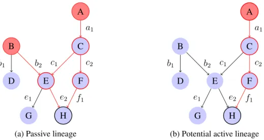
Following this, we are not only observing isolated mapping rules but the sequence of map-pings and can make assumptions about their combined impact. For example mapmap-pings with contradicting conditions on data processing are individually seen both valid and relevant for lineage computation, but applied in sequence may exhaustively restrict the conveyance of data items. This potentially allows to reduce the number of followed paths significantly and gives us the chance to determine the lineage of data even more accurately by excluding false pos-itives. Figure 3.1 illustrates the potential benefit of active lineage for theoretical data flows. Assuming we are interested in the lineage of items in H, the evaluated paths and resulting golden sources are painted red. In the case that both sequences of mappingse2 b2ande2 c2

could be excluded based on the logic in the respective mappings, source B can be identified as a false positive. Passive lineage, however, evaluates only the static data flows and therefore includes B as a golden source.

The system to be built uses the already existing rules about the structure of mappings, that are given in the form of a context-free grammar. By using those grammar rules, it is possible to

(13)

generate a generic system that filters the path according to certain criteria such as particular value ranges or attributes. Those filters may be user specified or a result of active lineage computations. To achieve that, there are two basic steps necessary:

1. Extract logic and meta information from mappings 2. Traverse the graph according to those results

We will explain both steps in great detail and then take a look at common patterns that occur during graph traversal based on the results. Additionally we will present a prototype that implements the results of our considerations as an empirical proof of concept. Finally there is an outlook on the possible extensions of the system as well as its current limits, especially in regard to the developed algorithm and the underlying system.

3.2. Lineage Specification

In order to explain our solution for the given task, we first need to elaborate on the possible degrees of lineage computations. We distinguish two types of lineage for our purposes: the

passive lineageandactive lineage. What we want to offer to the user is the more advanced active lineage. In chapter 4 we will compare those two forms of lineage to other common definitions.

Passive Lineage

Passive lineage denotes the more basic, static computation of data lineage. It finds all poten-tial sources of data items for a sequence of transformations. However, it does not consider further conditions or constraints that are given for data flows and therefore includes sources that effectively do not contribute to the result. For example data flows that are restricted through exclusive transformation rules may still be listed in passive lineage, even if no data item reaches the result table.

Let us consider the given database in 3.2 where we apply to both tables queryQ: Q:SELECT b.X, a.Z FROM A a, B b WHERE a.X = b.X AND b.V =v1

Now we are interested in the passive lineage of the result. For this it is sufficient to find the exact location from where data items were copied. Hence we look at Q and find that the SELECT statement reads both A and B but returns only data from A. This is apparent from the fragment "a.X, a.Z". Therefore we identify the passive lineage to be{A1}.

Additionally we consider another query Q2 which produces the same result but by different

means:

Q2 :SELECT b.X, a.Z FROM A a, B b WHERE a.X = b.X AND b.V =v1

(14)

A B C D E F H G b1 b2 e1 e2 c1 a1 c2 f1

(a) Passive lineage

A B C D E F H G b1 b2 e1 e2 c1 a1 c2 f1

(b) Potential active lineage

Figure 3.1.: Active lineage may reduce the lineage paths (red) for data items in H.

Active Lineage

In contrast, active lineage actively computes the conditions that need to be fulfilled in order to include a source in the lineage. This potentially reduces the number of sources, for example if an accumulated set of conditions along the way evaluates tofalsefor a particular source. In the end, active lineage is effectively the passive lineage with evaluated conditions on the data flow. Let us consider the given database in figure 3.2 and again apply queryQ, then the active lineage results in{A1, B1}with the attached conditiona.X = b.X ANDb.V = v1. We call

such an effective source of data agolden source.

Definition 1 While a source may be in general both target and data source for transforma-tions, agolden source is a source that serves only as data source and is not targeted by any transformation.

This makes the golden source the storage location of some or all of the original data items which were used in the computation of the given result. It does however not include sources that occur solely in conditional parts of the transformation.

Furthermore a source is only a golden source if its data items may in fact be part of the result and are not logically excluded by a combination of transformation steps beforehand. However, a golden source is not determined by the actual values of data items. An empty source may still be a golden source.

A X Y Z A1: x1 y1 z1 A2: x2 y2 z2 B X U V B1: x1 u1 v1 B2: x1 u2 v1 B3: x3 u3 v3 Result ofQ X Z x1 z1

(15)

4. Related Work

The following sections present the most common categorizations used in other works. We provide the reader an overview of the scope of similar procedures and how our approach, as outlined in chapter 3, relates to those.

While there exist many different ideas on how to solve the data lineage question, we go with a new and innovative approach. As described in the use case, the ultimate goal is to offer a service for users who have little or no knowledge in the technical area, but are interested in the lineage of data for further analysis. This makes a huge difference to other approaches, where the user may be required to understand the process in order to produce results. For instance Karvounarakis et al. use a custom query language in order to pose requests to the system [KIT10]. Glavic et al. designed their provenance systemPermas an extension of the PostgreSQL DBMS and expect the user to execute SQL queries for provenance information [GA09].

Furthermore most of the existing lineage algorithms work on the assumption that the actual content of the database is known and available. They trace or record real transformations by running them, like Cui et al. do in their work on lineage tracing in data warehouse transforma-tions [CW03]. But we have only access to structural information about transformatransforma-tions, not the transformed data. Therefore we do not only record the lineage at run-time, but evaluate the computational steps based on the structural information.

Regarding common terminology, it can be noted that many works use data provenance as synonym to data lineage [Tan07] or also pedigree [GD07, BT07]. Moreover it is a common approach to define three major categorizations for provenance information. Those are tradi-tionally why-, and where-provenance [BKWC01] as well as how-provenance in later works [CCT09, GM11]. Every category aims to find out a specific form of provenance. In order to classify our approach we will shortly describe the main differences between each of those categories.

Why-Provenance

The search for why-provenance leads to thecontributing source, orwitnesses basisas others call it [CCT09, GD07]. Why-provenance captures all source data that had some influence on the existence of the examined data item. Intuitively it explainswhyany data item is part of the result. This does not only include the actual data that is present in the result, but also data items that have to be used in order to select the final data. But even though many data items might be part of the computation (the set of witnesses), why-provenance denotes only the minimal set of data items that is necessary to produce the result (the witness basis). A simple example would be the following scenario: Take again two tables A and B as shown in figure 3.2.

(16)

For a given query like

Q:SELECT a.X, a.Z FROM A a, B b WHERE a.X = b.X AND b.V =v1

we get the result that is presented in the figure. Now we can immediately see that the origin of the result is solely table A, more preciselyA1. But according to the given explanation, we have

to include bothB1andB2into our consideration, since they were used by the query. However,

there is no need for both of them to exist in order to derive the same result. EitherB1 orB2

would suffice. Therefore the witness basis, i.e. why-provenance ofC1can be expressed as the

set{{A1, B1},{A1, B2)}}. For our goal to provide active lineage, we apply some of the same

operations that are also necessary to compute why-provenance. But instead of simply stating the why-provenance, we evaluate it after each step and draw further conclusions regarding relevance of sources. This concept is used in the preservation of conditions (chapter 6.3.1).

Where-Provenance

In contrast to why-provenance the where-provenance, also calledoriginal source, focuses on the concrete origin of data [GD07]. It respectively answers the questionwhere exactly data items come from, regardless of the reasons why they are part of the result. This relates strongly to our definition of passive lineage. While we need to compute the while provenance as a part of active lineage, it is not sufficient. We basically evaluate the why-provenance for each item in the where-provenance and then remove non-relevant items from the result.

How-Provenance

The concept of how-provenance is relatively new compared to the other two provenance types. It was introduced for the first time in 2007 by Green et al. [GKT07]. Following the nomen-clature of why- and where-provenance, how-provenance answers the questionshowthe result was produced andhowdata items contribute. It is easily confused with why-provenance, but goes one step further.

In order to record why-provenance, most systems use a special notation. In order to keep the introduction short, we relinquish the in-depth explanation of such a notation as it can be found in [GKT07] and [CCT09]. But by using the given example from figure 3.2 and again apply-ing queryQ2, we can also derive the (in this case) very simple how-provenance. The result

is a combination of two tuplesA1 ^B1, effectively preserving the computational expression

that was used. By following such provenance information through the set of transformations, we get a picture not only where data items come from, why they are part of the result but also how exactly they were computed in each step. This is definitely the most advanced and thorough type of provenance. For our purposes however this yields no advantage over active provenance. It is not important for us how the data was computed, only the fact that the com-putation allows for its contribution to the result.

To summarize, our goal is ultimately to compute active lineage in contrast to other systems that process only one of the previously presented provenance categories. We do not only

(17)

follow along the lineage path, but also use the gathered information to dynamically decide which paths and sources are effectively relevant for the lineage. Furthermore we want to provide the user with complete abstraction from the processing, which distinguishes our work from most of the other systems that require advanced user-interaction.

(18)

5. Approach

Now that we have outlined the task and how we want to approach it, we first need to intro-duce some of the tools that we have defined before we can start in-depth explanations of the developed algorithm in chapter 6. We will therefore address the definition of mappings as mentioned in chapter 2, as well as the grammar and the generic graph representations.

5.1. Mapping

The basic element that we use in this work is a mapping. While the meaning of "mapping" can differ depending on the context, we follow the definition used by Credit Suisse, which is also incorporated in existing works:

Definition 2 A Mapping is a set of components that are used to describe the creation of rows in a target table. They contain descriptions of rules and transformations that have to be applied in order to move data from one area to another one in the required form.

It is basically used for three purposes:

1. To specify the elements that are necessary to create rows in a given database table (e.g. other tables, columns, values).

2. To specify how to manipulate and transform those elements under certain conditions. 3. To document the whole process.

A concrete example of such a mapping is given in figure 5.1. In accordance to the defini-tion, it describes the mapping of columns from tableCUSTOMER_MASTER_DATAto table

AGREEMENT and provides instructions on how to transform elements under different cir-cumstances.

Mappings are a very powerful tool to describe those transformations. They include not only data flows inside of single databases, such that pure SQL statements could cover. Mappings can specify how data is moved from database to database within the data-warehouse, or how to populate a table from flat files based on a given file structure. The mapping description as part of the metadata is not concerned with concrete implementations and therefore can express the complete data flow on a conceptual level.

There exist various mapping components that can be part of a mapping. They include for example elements such asEntity, Attribute, Entity Attribute Population, Entity Attribute Population Condition Component and many more. Every component is represented in the

(19)

WHEN POPULATINGEntity: AGREEMENT

FROMEntity: CUSTOMER_MASTER_DATA

POPULATEAttribute: AGREEMENT.ACCOUNT_CLOSE_DT

WITHCUSTOMER_MASTER_DATA.LAST_ACCOUNT_CLOSING_DATEIF

CUSTOMER_MASTER_DATA.LAST_ACCOUNT_CLOSING_DATE != 01.01.0001 WITH"DEFAULT MAX"

POPULATEAttribute: AGREEMENT.ACCOUNT_FIRST_RELATIONSHIP_DT

WITHCUSTOMER_MASTER_DATA.FIRST_ACCOUNT_OPENING_DATEIF

CUSTOMER_MASTER_DATA.FIRST_ACCOUNT_OPENING_DATE != 01.01.0001 WITH"DEFAULT MIN"

POPULATEAttribute: AGREEMENT.ACCOUNT_OPEN_DT

WITHCUSTOMER_MASTER_DATA.CIF_OPENING_DATEIF

CUSTOMER_MASTER_DATA.CIF_OPENING_DATE != 01.01.0001 WITH"DEFAULT UNKNOWN"

Figure 5.1.: Real world example of a mapping from CUSTOMER_MASTER_DATA to

AGREEMENT.

conceptual mapping data model, designed by Credit Suisse experts. Themapping data model

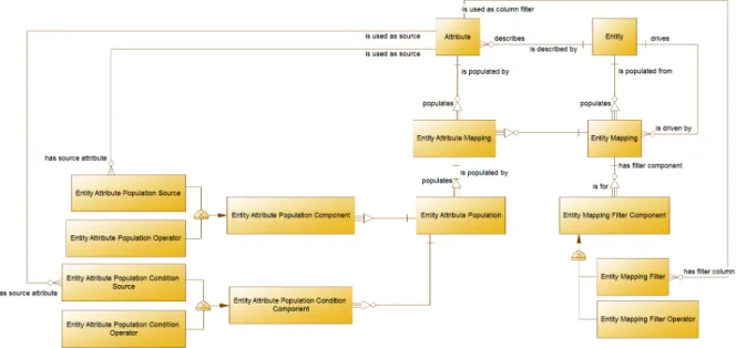
"describes the data required to document the population of Entities (Feeder Files, Tables, etc) and to provide a means for reporting data lineage" [Bud12]. This model includes every element that is needed to express any mapping within the given system. That means that every mapping can be constructed using only components from the model. A simplified excerpt is shown in figure 5.2 (see appendix A for the full model). It can be seen as a blueprint for mappings and therefore served as an important basis for our work.

The mapping data model describes data sources and targets of mappings as entities, which are in our case tables in the underlying database system. Similarly the entity’s attributes are columns of the table. Each of those entities can potentially be both source and target. Therefore we call those entities generallysource (of a mapping) and refer to them astarget

only in the explicit case for a specific transformation to avoid confusion. However, we use

entityandattributewhen describing more conceptual ideas.

5.2. Grammar

However, instead of working with the data model from section 5.1, we utilze the existing formal context-free grammar (see figure 5.3) that is based on the model. It describes the struc-ture of any mapping in accordance to the mapping data model and includes all elements that were specified there. Consequently it is it sufficient to express every possible composition of mapping components in the given syntax (see appendix B for the full grammar). Mappings

(20)

Figure 5.2.: Excerpt from the conceptual data model for mappings

written in this form are meant to be human readable and therefore more verbose than tech-nically necessary. A user should be able to understand the meaning of the mapping without further reference material. At the same time they can be processed by a computer, since they are structured according to the given grammar rules, unlike natural language. Figure 5.1 from the last section is written according to this syntax.

In order to use the grammar for our purposes, it was expedient to change the structure of some production rules so that we can represent these rules in a tree structure. This is far more convenient than a relational representation, as we will explain in section 5.3 in more detail. From this it follows that the grammar is not only used for its traditional purpose only, namely parsing input, since we plan to use already well-structured data. Mainly it is used as a basis for further processing of the mapping, independent from the technical implementation of any input.

mapping ::= population filter? navigation? population ::= WHEN POPULATING targetEntity

FROM drivingEntity populationClause populationClause ::= (POPULATE populationComp)*

populationComp ::= attribute withClause+

withClause ::= WITH expression (IF condition)? expression ::= string | computation | concatenation

(21)

5.3. Grammar And Model In Comparison

To explain why we decided to use the grammar as a basis for our computations, we now com-pare the grammar with the model to show similarities and argue how the grammar is superior for our purposes.

First of all, the grammar is suited to give a human reader, who has no knowledge of technical details, insight on the content of mappings. It defines a syntax and allows a human reader to deduce the purpose of a component based on its written context. For example does the mapping always include exactly one main source and one target entity. The data model in figure 5.2 represents this with two relations betweenEntity and Entity Mapping. An Entity Mapping"is driven" by exactly oneEntity, which makes that the declared main source for the mapping. Similarly exactly oneEntity"is populated from" theEntity Mapping, which makes thisEntitythe target. But given only the relational tables, it is difficult for a human to derive which is a source or a target. It is necessary to follow the respective keys in the physical mapping table and therefore to have technical knowledge about the concept of databases. The grammar, however, attaches semantic meaning to each element with the syntax and provides needed context regardless of any technical implementation. Considering a mapping such as in figure 5.1, let us examine at the first lines:

By comparing this to the rule "population" in the given grammar from figure 5.3, we can im-mediately identify the main source asCUSTOMER_MASTER_DATA and the target table as

AGREEMENT.

Now one could argue that apart from readability both model and grammar are equal in power and coverage and therefore we could also use the model for our lineage computations. However, the latter is a far more suitable tool for our purposes. The reasoning for that is the following:

It is definitely possible to describe a mapping with the data model as well as with the gram-mar. Both define the structure of the mapping and determine how to compose the elements. However, the grammar is built hierarchically, whereas the model is flat, as it is meant to be implemented in a database system and can be directly converted into a relational table schema. This gives the grammar an advantage since we want to work on graph structures, as has been stated in chapter 2. A mapping can therefore be extracted directly from the underlying map-ping graph in a graph representation, in contrast to a relational representation.

We gain then further advantages over a relational model when processing mappings in tree form. For example recursive rules, such as groupings or computations that are part of other computations can be traversed easily in a hierarchical representation, but on a relational schema this would lead to multiple self-joins of potentially very large tables.

Additionally, the grammar allows to easily validate given mappings. Parsing an error prone input is immediately noticed, whereas the population of tables may include many unknown

(22)

mistakes. Although this does concern the input of mappings more than the lineage compu-tations, it played an important role in the decision to devise a grammar. Since therefore all mappings are in a form compatible to the grammar, we can perfectly use it to describe the general structure of mappings.

To conclude this argumentation, we can summarize that the model is perfect to represent data in a relational schema that is only accessed by computers. However, once human interac-tion is necessary, the grammar offers superior comprehensibility. Addiinterac-tionally, the hierarchical structure offers easier integration into the graph based system on which we are building our solution.

5.4. Utilization Of The Grammar

After we have shown that it is beneficial to use the grammar as a basis for our system, we now explain how we utilize the grammar.

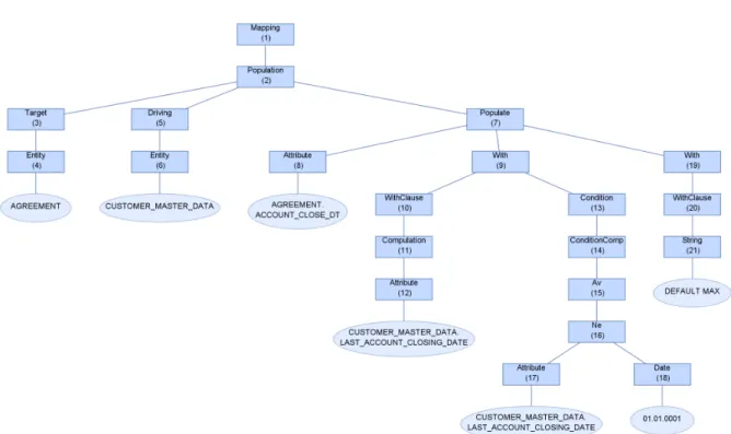
For one, the grammar defines how concrete instances of mapping trees are structured. The im-portant requirement we set for those tree representations is that no semantic information may be lost during tree construction, it must be possible to unambiguously recreate the mapping. For instance it is necessary to distinguish between source table and target table, not just to include two equal tables. Therefore we include targetEntityand drivingEntity, as figure 5.3 illustrates. We also need to preserve the mathematical computations according to the order of operation rules instead of order of appearance and similar information. Our grammar fulfills this requirement since it is completely compatible to the data model, as we explained in sec-tion 5.2. For a given mapping as in figure 5.4, the corresponding tree representasec-tion according to the grammar is shown in figure 5.5.

Consequently the grammar rules enable us to create a "map" of all components that may be part of a mapping. Looking at the grammar, we can immediately see where attributes occur or where computations may be used. Without this map, we would have to rely on actual instances of data to get a grasp of the structure on a per-mapping basis. However, we want to present an algorithm that works universally on any mapping. Therefore we can not rely on concrete data items, but have to work with the abstract mapping structure and then apply the resulting strategy to the concrete instances. Once this structure is known, we can determine all possible compositions of mappings beforehand and define algorithms universally for every mapping in the system.

The great advantage in this approach lies in the opportunity to use this to search not only for elements by occurrence but also by semantic meaning. We are for instance able to look specif-ically for the target table instead of any occurrence of a table, since we can exactly determine how and where it is specified in a mapping.

(23)

CUSTOMER_MASTER_DATA.LAST_ACCOUNT_CLOSING_DATE != 01.01.0001 WITH"DEFAULT MAX"

Figure 5.4.: Simple example mapping

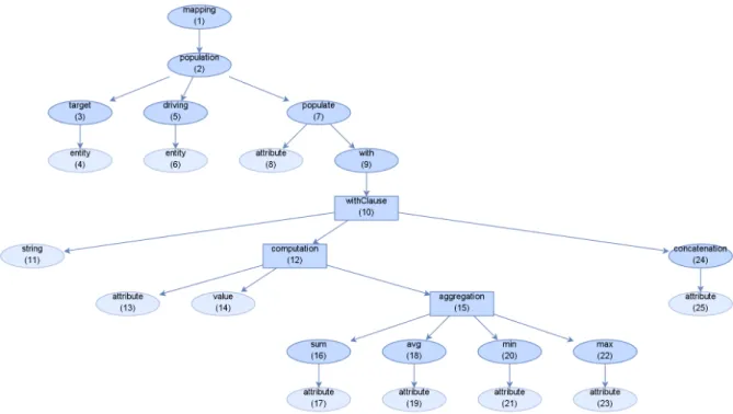
Figure 5.5.: Parse tree built from a simple mapping. Nodes are represented as squares, the content of leaf nodes is attached as an oval shape. Numbers in brackets denote the Id of each node for quicker reference.

(24)

6. Lineage Computation

Having explained the concepts that we use in our system, we can now commence with the in-depth explanation of the algorithm.

In order to answer a given question such as the request for the golden sources, we generally have to convert the input into a set of computations. For this we must address two basic aspects. Firstly it is necessary to follow the paths through the system and therefore to navigate from one intermediate source to the next by selecting all appropriate mappings, as we will describe in section 6.1. This is a high level process and can be expressed by a query over the set of all mappings. However, to identify those relevant mappings, we need to retrieve information from each mapping separately. Using those results is a more complex and requires different data depending on the posed request. This will be addressed in section 6.2. Secondly, to avoid false positives, it is necessary to preserve possibly stronger constraints in population conditions after each step. Section 6.3.1 will explain this aspect in more detail. It should be noted that by dividing the algorithm into several modular steps, we offer the basis for other investigations that were mentioned in chapter 2, such as impact analysis. Depending on the type of the request it is possible to retrieve different information from each mapping with a generic query. The affected parts of the algorithm can then be adapted for different situations, while the remaining implementation stays intact. However, we will focus purely on the data lineage aspects in this thesis, as it has been stated in the task description in chapter 3.

6.1. Moving Along The Graph

We already explained in section 3 that the main goal is to determine the lineage of a given data item all the way back through the graph of mappings. This eventually leads back to one or more golden sources. We therefore call this concatenation of mappings the lineage path in the mapping graph. Note that a source for one mapping can also be the target for another mapping.

Mapping Graph

Themapping graph M G(S, M) is composed of vertices S := _{s0, s1, ..., si} and directed

edgesM := _{m0, m1, ..., mj}, i, j 2 N. S is the set of all sources andM is the set of all

mappings which are present in the system. where|S| 2and|M| 1.

An edgemk=hsm, sniis considered to be directed fromsmtosnforsm, sn 2S.

Using the previously explained mapping data model we can deduct the following property: Each mapping always contains exactly one source and one target entity. Therefore we can definesm to be thesourceandsnto be thetargetof the mappingmk.

(25)

Lineage Path

Thelineage pathis a subset of mappingsL_✓M in the mapping graph. It describes the path that a data item took in the mapping graph from the golden source up to the user specified target, i.e. the set of mappings that were used during the computation of the result.

To find the lineage path, we need to navigate from the final result back in the mapping graph step by step and follow the edges in reverse order from source to source. We need to execute the same process recursively, until we reach the end of each path, i.e. the golden source. This algorithm can be roughly outlined as follows:

1. Find all mappings that use the current source as target 2. Extract the responsible sources from each of those mappings 3. Preserve the constraints for each source

4. Treat each result from step 2 as new target and continue with step 1 until no more mappings can be found

The first step can be expressed in one simple query over the set of all mappings and results in a set of zero or more mappings. Since we start with one single item, we select this item as starting point in the mapping graph and move on from that.

But it is not sufficient to follow the lineage paths on the entity level as one would assume intuitively. Each attribute can be populated from numerous sources. So we need to follow the lineage path explicitly for each attribute. Following that, the second step needs therefore to return a list of all source attributes that populate the corresponding target attributes. This can be achieved with a separate algorithm which is explained in the next chapter. After retrieving the source attributes, we then need to make sure that no false positives are included in the path. This is an important part of our approach and one of the key features. We therefore collect and process any constraints on the attribute level for every lineage path. Detailed explanation of this issue follows shortly.

6.2. Extracting Information From Mappings

As explained in 6.1 it is necessary to extract some information from each mapping according to the results from the last step. In this case we are generally interested in the same elements of a mapping in every iteration, but it is very likely that every mapping is structured differently than the one before. Therefore we cannot re-use the same static query over and over again, but have to make adaptations to the parameters and cater for any feasibly mapping structure. In order to formulate those queries, we have to follow several intermediate steps and consider several factors. In a simple implementation, the user might need to work some of this parts out on her own. However, in our scenario, the user cannot be expected to have extensive knowledge about both the mapping structure and database systems. Therefore we offer a high

(26)

degree of abstraction. That leaves us in a position where we have to interpret the input and then generate the corresponding queries automatically from that. However, we do not want to constrain the user with limited power of the system. As a result, the now proposed algorithm is more than just a necessary tool to compute data lineage. It is a general solution to extract information from mappings while considering the semantic meaning of each element. This might prove very useful when addressing similar issues as later described in chapter 9, where we are interested in other components of the mapping.

The first challenge is to create some kind of processable mapping blueprint, that gives us an idea of the structure of a mapping. We can then find out which elements we are interested in and where to find them. This part of the process can be re-used in every iteration. The next step is the extraction of information from the specific mapping at hand where given parameters are used to find matching elements as output.

Before we can describe the algorithm in detail, it is necessary to explain some of the used constructs and definitions.

6.2.1. Meta Tree

As a basis for the process of data retrieval from mappings, we introduce the so-called meta tree. This is a simplified representation of the grammar rules in graph form, which describes what the instance graphs of mappings parsed with the grammar can possibly look like. To support the tree representation, the changes to the grammar that are mentioned in section 5.2 were made. We normalized the rules in such way that now every rule is either a composition of several other rules or a set of mutually exclusive alternatives. Therefore we can now distin-guish between two cases: the compositions of rules and the list of alternative rules.

Rules in the form of

aggregation ::= ’SUM(’attribute’)’ | ’AVG(’attribute’)’ | ’MIN(’attribute’)’ | ’MAX(’ attribute’)’;

are calledalternative rules. There can be only one alternative element selected at a time and each alternative element may consist of only one component. In contrast, rules in the form of

navigation ::= ’NAVIGATE’ fromEntity ’TO’ toEntity ’USING’ (usingClause)+;

are calledcomposition rules. Every non-terminal symbol on the right hand side of a compo-sition rule is element of the same alternative and the compocompo-sition rule itself may contain only a single alternative.

(27)

We made two simplifications in the transformation of the grammar to the meta tree. This happens in order to construct a tree and not just a directed graph with possibly cycles. The first simplification therefore attacks recursive rules. Such a rule is for examplecondition:

condition ::= multiCondition (condComponent)* ; condComponent ::= andOrOperator multiCondition;

We reduce those rules by ignoring the recursive element. The condition rule is instead as-sumed to be equal to

condition ::= multiCondition;

The reason for this follows the purpose of the meta tree. We want to create a map of possible occurrences of certain elements. While a condition may be a sequence of other conditions that are linked with AND or OR statements, we are interested only in the fact that an attribute may be part of a condition, not where specifically in the recursive chain of condition it is located, i.e. on which level of the tree.

Second, compositions of equivalent non-terminal symbols such as concatenation ::= attribute ’||’ attribute;

are considered to be equal to the reduced composition rule concatenation ::= attribute;

Again, we only need to know that an attribute may be part of a concatenation, not if it is the first or second element.

The tree representation according to this hierarchical structure of the grammar rules is the meta tree.

Definition 3 Themeta treeis a graph MT(R,E) with a set of verticesR :={r0, r1, ..., ri}and

directed edgesE :=_{e0, e1, . . . , ej},i, j 2Nwhere|E| 0and|R| 1.

Ris considered to be the set of all rules in the grammar. Those can either be alternative rules or composition rules. ri denotes the i-th rule in the grammar and is therefore represented in

the meta tree as node with Id i, i.e. Id(ri) = i. E is the set of all edges that represent the

hierarchy of grammar rules. An edgeek =hrm, rniis considered to be directed fromrm torn

forrm, rn 2 R. Edges connect a grammar rulerm with each non-terminal symbolrnon the

right hand side of the rule. The root of the tree is alwaysr0, i.e. the first grammar rule.

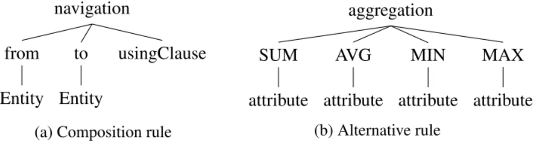
As an example let us have a look at the mentioned composition rulenavigationand alterna-tive ruleaggregation. The tree representation of thenavigationrule can be seen in figure 6.1a and similar figure 6.1b illustrates theaggregationrule. Figure 6.2 shows an larger excerpt of the full meta tree, whereaggregationin incorporated.

(28)

navigation usingClause to Entity from Entity

(a) Composition rule

aggregation MAX attribute MIN attribute AVG attribute SUM attribute (b) Alternative rule

Figure 6.1.: Example for meta tree construction

In a grammar, every production rule is eventually resolved to one or more terminal symbols. In the same way a parse tree contains only terminal symbols in leaf nodes. Since our meta tree does not visualize an actual input but merely the allowed structure, similar to the plain grammar, we include all non-terminal rules and not the terminals themselves. The nodes that form our leafs are therefore: entity, attribute, string, value and date. With this structure, we have now created a map to locate individual parameters for our blueprint query within their respective contexts.

If we want for example check every mapping that uses a certain value, we can immediately see in the meta tree where exactly a value may occur. In the example, this would be only one place, as part of a computation in the withClause. So without any further action, we immedi-ately know exactly where we have to look for a value in mappings and its context.

The meta tree is not to be confused with the abstract syntax tree (AST) or the parse tree. While the AST and parse tree both display a concrete instance of the rules, we have created a generic presentation of the rules independent from any input. For example a computation in a parse tree can contain another computation and several values, while the meta tree only indicates the possible existence of a computation. The important information stored in the meta tree is the possibility of an occurrence of the computation at this position and therefore its context.

6.2.2. Affected Leafs

Once the meta tree is established, it allows us to select the parameters for the query. Possible examples for parameters are very specific requests, such as

"get all occurrences of ’5’ as value in a computation within the withClause" (I) "get all occurrences ofAGREEMENT.ACCOUNT_CLOSE_DTin a population" (II) While (I) is a very specific parameter and can be directly resolved, the second request (II) is more general and needs some processing. By using the meta tree as it is displayed in 6.2, we can identify the relevant leaf nodes in both cases. Imagine the request is positioned at

(29)

Figure 6.2.: Part of the meta tree built from the grammar rules. Oval nodes represent compo-sition rules, square nodes alternative rules. Numbers in brackets denote the node id for more convenient references.

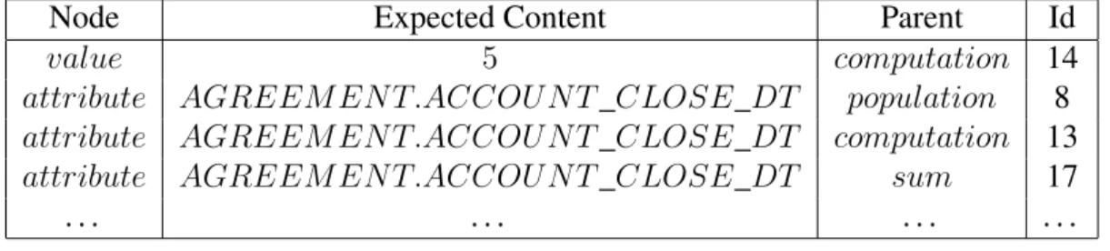
the given node in the tree, i.e. (I) at the corresponding ’value’ node with Id 14, (II) at the ’population’ node with Id 2. When traversing the subtree with the selected node as root, we visit all leaf nodes and add the appropriate leafs as well as their expected content to a list of matches. This has to be done for each parameter and results in one list of parameterized nodes. In the case of (I) this is easy, since we get a subtree with only a single node. Here ’value’ (14) is already a leaf so we add it to the list and are done. For (II) this requires a more complex reasoning. Starting from the ’population’ (2) node, we find 7 leafs of type ’attribute’. One directly as target of the populate (7) clause, 5 of them within a computation (12) and another one in concatenation (24). Thus we get a total of 9 parameterized nodes for the two example requests (I) and (II). An excerpt from the list of matching nodes after the process was executed is shown in Table 6.1. To simplify the description of requests, we propose the following short notation for the selection of parameters:

context Id, node type, expected content

For instance the two previous examples can be expressed as

10, value, 5 (I)

(30)

Node Expected Content Parent Id

value 5 computation 14

attribute AGREEM EN T.ACCOU N T_CLOSE_DT population 8

attribute AGREEM EN T.ACCOU N T_CLOSE_DT computation 13

attribute AGREEM EN T.ACCOU N T_CLOSE_DT sum 17

. . . .

Table 6.1.: Parameterized Nodes

6.2.3. Computing The Context

To correctly identify all involved leaf nodes in the actual parse tree later on, we need to make sure that we can identify the semantic meaning of every node. For a given set of nodes in the parse treeP = _{p0, p1, ..., pi}, i 2 Nand nodes in the meta treeR = {r0, r1, ..., rj}, j 2 N

we define

Definition 4 The semantic context(Contexts) of a leaf node pn, n 2 N in the parse tree

describes the exact position of its semantic representationrm, m 2 N in the meta tree. This

may be expressed with the unique Id of the noderm.

This is equal to the n:1 mapping defined by8p2P 9r2R: Contexts(p) =Id(r)that maps

each leaf in the parse tree to one leaf in the meta tree. In other words, the semantic context shows the semantic circumstances of the usage of a nodepi. For example the context of the

target entityAGREEMENT in the parse tree in figure 5.5 is 4, as can be seen in the meta tree in figure 6.2. ThereforeContexts(p5) = 4.

In order to compute the semantic context Contexts(pi), we need to utilize another tool, the

set of identifying ancestors.

Definition 5 Anidentifying ancestoris a non-leaf node in the meta tree that necessarily has to exist exactly once in the set of ancestors for a given node in the meta tree.

This includes every ancestor in the meta tree, where the corresponding grammar rule does not start and is not part of any recursion. Each identifying ancestor is used to unambiguously identify the semantic context of the succeeding nodes.

We consider IA(rn) = {ri, ..., rj}, i, j 2 N to be the set of all identifying ancestors of rk,

k ₂ N in the meta tree. In contrastallAncestors(x), x ₂ P _{_}x ₂ R describes the set of all ancestors of nodex, including those that are not identifying ancestors forx 2 R. We write isIdentif ying(ri),i2Nto express the fact thatri is an identifying ancestor.

To underline this definition, we look at a simple example in our meta tree in figure 6.2. The set of identifying ancestors IA(r14) = {r10, r9, r7, r2, r1}. Node r12 is not part of the set of

identifying ancestors, since computations may occur recursively.

Furthermore we introduce thecomputational context(Contextc) of a leaf nodepas follows:

Let beC ={r0, r1, ...},C ✓R^ 8ri 2C :isIdentif ying(ri) =true, further

(31)

j =Contexts(pj).

Then we can sayContextc(pn) =rk |k =Contexts(pl),pl 2D,rk 2R.

From those definitions, we can make the following deductions:

• Contextc(pi)= IA(rj),j = Id(Contexts(pi))

• Contextc(pi)=Contextc(pj),Contexts(pi)=Contexts(pj)

Using those, we can now compute the semantic context as

Contexts(px)= Id(ry)|ry 2R,Contextc(px) = IA(ry),y=Contexts(px)

As an example, let us look at the parse tree and consider the node Attribute with Id 12 and content CUSTOMER_MASTER_DATA.LAST_ACCOUNT_CLOSING_DATE. According to the presented definitions, we can compute Contexts(p12) = 13, since the corresponding

node in the meta tree isr13.

With those tools at hand, we can now generically compute and compare the context of each node in the parse tree. This is an advantage, since we do not need to take the actual structure of the current tree into consideration, but have defined a general solution that works for every possible parse tree and therefore every possible mapping.

6.2.4. Select Data

In this step we now load the actual data from a mapping according to the parameters selected in 6.2.2. To find matching data items in the parse tree, we need to consider and check for two properties of every data item:

1. Node type and content 2. Semantic context

This is reflected in our proposed notation from section 6.2.2. It is necessary to consider those properties, since not every occurrence of a given node content happens in the same type of node. For instance the contentAGREEMENT may occur as an entity with this name or as a simple string without computational value. Depending on the situation we may be interested in only one of both manifestations, say the entity. Now an entity may be used in several dif-ferent contexts, which we also have to distinguish. In the given sample from the meta tree in figure 6.2 entity may occur with the semantic context 4 and 6, i.e. as target or source. But if we are looking only for a target entity, the entity with semantic context 6 is not relevant.

We assume as a simple example that we are given the same mapping as in figure 5.4. Let us say we are now interested in the request

(32)

That means, we want to see where attribute LAST_ACCOUNT_CLOSING_DATE of table

CUSTOMER_MASTER_DATAis used as component of an population that in turn is used to populate another attribute. Figure 6.3 shows the matching attribute in bold.

CUSTOMER_MASTER_DATA.LAST_ACCOUNT_CLOSING_DATE != 01.01.0001

WITH"DEFAULT MAX"

Figure 6.3.: Simple example mapping. The attribute of interest is written in bold. However, as can be seen in both figure 6.3 and 5.5, this attribute occurs at two different locations, once in a with clause and once as part of a condition. Yet we are only interested in the first one.

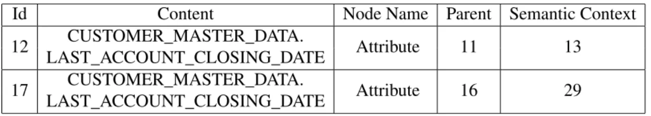
As explained, we have to determine all relevant leaf-nodes in the parse tree first and then check the semantic context of those in order to eliminate the false positive. The first step is to query for any occurrence ofLAST_ACCOUNT_CLOSING_DATE. The result is shown in table 6.2 and contains both of the mentioned nodes.

Id Content Node Name Parent Semantic Context

12 _{LAST_ACCOUNT_CLOSING_DATE}CUSTOMER_MASTER_DATA. Attribute 11 13 17 _{LAST_ACCOUNT_CLOSING_DATE}CUSTOMER_MASTER_DATA. Attribute 16 29

Table 6.2.: Result of the query and the respective semantic context of each node The semantic context of each node was added manually for a better overview. The calcula-tion of the semantic context for each element in the parse tree was outlined in 6.2.1 and won’t be repeated here. It is now easy to see that both elements are used in a different semantic context. We can gather from the meta tree that the semantic context that we are interested in is 8, taken from the Id of the corresponding node. By comparing the semantic context of each node with the relevant semantic context, we can see that only one node remains. This is our final result in this step and shown in figure 6.3.

Id Content Node Name Parent

12 _{LAST_ACCOUNT_CLOSING_DATE}CUSTOMER_MASTER_DATA. Attribute 11 Table 6.3.: Result from the data selection

(33)

6.2.5. Compose Data And Project Result

The previous section 6.2.4 showed how to extract elements from mappings. But since we are not only interested in the basic fact that a certain element exists in a mapping, but also how it relates to others, we offer a more complex query mechanism that can answer requests such as "get all attributes that occur in the semantic context 10 and are in the same population as the

attribute table0.attribute0 with semantic context 8 " We translate this request into the query

8, attribute, A : 10, attribute

The first parts defines the look-up, as explained before: an attribute in the semantic context 8 or below in the meta tree, with the content A. The second part defines the projection from the mapping to all attributes with or below the semantic context 10, independent from their respective content. We assume implicitly that both should besemantically relatedin such way that they are both used in the same part of a mapping. In this case, we are looking for pairs of attributes that occur in the same population, not just in any population clause. One should have the given semantic context and content, the other is within a given semantic context and can have any content. To explain this relation formally, we need to introduce the following notations:

Thelowest common identifying ancestor(LCIA) of two nodesp, q 2R, where R is the set of all nodes in the meta tree, is the lowest common ancestor ofpandqthat is identifying, i.e. r=lca(p, q)_^isIdentif ying(r) =true, or shortr=lcia(p, q).

Two elementsp, q₂ P where P is the set of all nodes in the parse tree are said to be

seman-tically relatedin the lowest common identifying ancestor rrelated, or shorter in the semantic

contextId(rrelated), if the following set of conditions hold:

1. Contextc(pi)\Contextc(pj)6=;

2. allAncestors(pi)\allAncestors(pj)6=;

Then we can say

1. rlcia =lcia(Contexts(pi), Contexts(pj))

2. A=allAncestors(pi)\allAncestors(pj)

With that we can derive the relevant common ancestor to be

pcommonforpcommon2A^Contexts(pcommon) =Id(rlcia)

and from that define

(34)

To apply this definition to an example, let us examine the mapping from figure 5.4, and pose the request

8, attribute,AGREEMENT.ACCOUNT_CLOSE_DT: 10, attribute

We can split this up into the two mentioned steps of executing the look-up and then the pro-jection.

Look-Up

By looking at the mapping tree in 5.5, we can see thatAGREEMENT.ACCOUNT_CLOSE_DT

occurs only once in the mapping as p8. Its semantic context computes as ContextS(p8) =

8, i.e. it is the attribute that gets populated by the population. We are looking exactly for attributes with context 8, therefore it is a match.

Projection

Now we consider the projection of results for the items found during the look-up. This means we have to look up all remaining attributes in the table and then check the context for each. Querying the tree for this delivers a small result set:

Id Content Node Name Parent

12 _{LAST_ACCOUNT_CLOSING_DATE}CUSTOMER_MASTER_DATA. Attribute 11 17 _{LAST_ACCOUNT_CLOSING_DATE}CUSTOMER_MASTER_DATA. Attribute 16

We are now able to compute both the computational and semantical context for all the at-tributes and find:

pi ContextS(pi) ContextC(pi)

p12 13 10, 9, 7, 2, 1

p17 29 15, 13, 9, 7, 2, 1

p8 8 7, 2, 1

Since we are interested only in attributes that are used in a sub-context of context 10, we can discard p17 since context 10 is not part of its computational context. The lowest common

identifying ancestor of the remaining attributep12and the givenp8can now be computed as

lcia(p12, p8) = 7

Expressed in natural language that meansp12andp8are both part of the same populate clause,

as stated in the initial request. This can be verified with a look at the mapping or parse tree. In terms of lineage calculations, we use exactly this type of request recursively. More general

(35)

8, attribute, X : 10, attribute

where X is a placeholder for the currently investigated attribute. This request lists all attributes that were used to populate the given attribute X. If we were interested in further lineage cal-culations for our example, we would now proceed withp12, find all mappings that populate

CUSTOMER_MASTER_DATA and run the query with the new found attribute on those, i.e.

8, attribute, CUSTOMER_MASTER_DATA.LAST_ACCOUNT_CLOSING_DATE : 10, attribute

6.3. Condition Evaluation

What we offered so far was the passive lineage of attributes. But one of the advantages of our approach is the incorporation of the logic behind each mapping, that leads us to active lineage. We therefore examine the conditions under which different data items are used for the computations. This allows to reduce the number of lineage paths in some cases, as we indicated in section 3. While each mapping may allow for a broad band of data items to be processed, a sequence of mappings potentially removes some attributes from the result by applying excluding conditions on populations. This is not necessarily an error in the design of mappings. Intermediate sources may be starting point for several different computations with different purposes and therefore serve as sources for many mappings that require different data.

We therefore collect conditions along the lineage path and evaluate them after every step. However, the selection of paths may be further restricted if the user has additional knowledge about the composition of attributes or wants to constrain the lineage on given properties. In order to provide this functionality, we differentiate between preserved conditions, which are a collection of conditions along the lineage path and the initial conditions, which are user specified.

6.3.1. Preserved Conditions

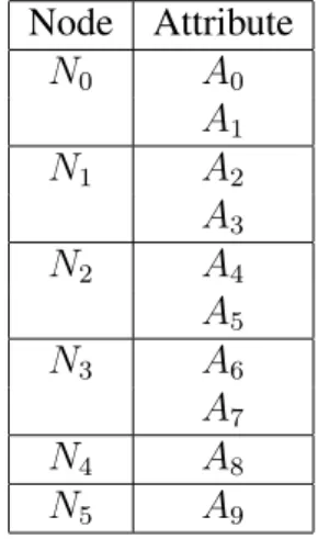
While traversing the mapping graph, we dynamically record and update the conditional logic according to previous steps. The usefulness of maintaining and updating the combined con-ditions along the lineage can be shown in a quick example. Imagine a scenario with five intermediate results which are represented in the graph as five nodesNi,0i 4where the

data flow is directed fromNn+1 toNnfor0 n  2. That means every attribute from Nn+1

has a corresponding source inNn. Additionally we insert a mapping fromN4 toN3 and one

fromN5toN3, but with slightly different properties, which will be defined shortly. Figure 6.4

(36)

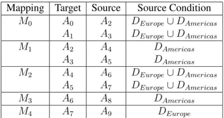
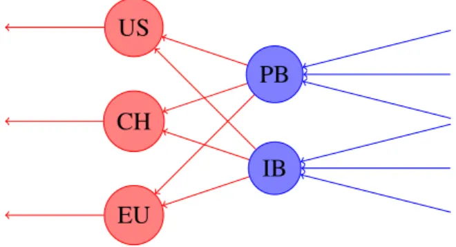
Mapping Target Source Source Condition M0 A0 A2 DEurope[DAmericas A1 A3 DEurope[DAmericas M1 A2 A4 DAmericas A3 A5 DAmericas M2 A4 A6 DEurope[DAmericas A5 A7 DEurope[DAmericas M3 A6 A8 DAmericas M4 A7 A9 DEurope

Table 6.4.: Mapping components in a population

Every mapping Mj, 0  j  4contains a set of mapping rules, or more specifically rules

about populations of certain attributes. Let us denote the attributes that are populated by those rules asAk,k = 0,1,2, . . .which we use as an arbitrary numeration to distinguish individual

attributes from several entities in this example. Table 6.5 shows a list of all exemplary nodes with their respective attributes.

In a mapping everyAk is provided with a condition Ck that adds a certain constraint which

has to hold true in order to allow the population to be executed. Let those constraints for instance be set in a way that they select a subsetDr of all data D for which the population

transformation is applied, with r ₂ _{Europe, Americas_}. This could be translated as a selection only consisting of data connected to a specific region. In Table 6.4 we can see the list of mapping elements to consider in this example. So in accordance with the grammar, the relevant part of the rules could be written as

. . . POPULATEA0WITHA2IFA2.REGION =EuropeOR

A2.REGION =Americas. . .

. . . POPULATEA1WITHA3IFA3.REGION =EuropeOR

A3.REGION =Americas. . .

. . .

Now let us assume we are interested in the lineage of the two data itemsA0 andA1 in the last

node, namelyN0. It is easy to see from the table that the source ofA0 isA2and the source of

A1isA3. On first glance it is sufficient to apply the initially given constraint about the region

within every following iteration, which dictates that data from both Europe and Americas is considered in both attribute populations. But if we follow the next step back fromN1 toN2

and then fromN2toN3while keeping that initial constraint, we will now start to include false

positives. M1 only relays data from Americas. Yet when processing M2, we again consider

data from Europe in further lineage inquisitions, even though the data contained inA0 andA1

is solely associated with Americas. At the lineage path junction inN3 we should therefore

follow M3 exclusively in further investigations and ignore M4. The same issue arises if we

instead apply only the current constraint of every population and not the initial one, as can be seen at the example ofM2 andM1.

Two conclusions can be drawn from those considerations. Mainly we have shown that it is vital to dynamically update the constraints after querying each mapping, rather than using the

(37)

Node Attribute N0 A0 A1 N1 A2 A3 N2 A4 A5 N3 A6 A7 N4 A8 N5 A9

Table 6.5.: Node attributes

N4 M3 ✏ ✏ N0oo _M0 N1oo _M1 N2oo _M2 N3 N5 M4 O O

Figure 6.4.: Visualization of nodes and mappings

static conditions in every population. If the last constraint is stronger than the one before, we only apply the last one and vice versa. This can be achieved by detecting the strongest con-dition after every step and then evaluating the aggregated concon-dition accordingly. Secondly it is obvious that we need to work on attribute level, since each attribute has to follow different constraints according to their individual population rules.

But how can we update the conditions properly? There are certain limitations, due to the se-mantic meaning of certain decisions. We include for example France as a region as part of Europe. A human user can intuitively understand that data from France might be included in a mapping for data from all of Europe, but not vice versa. To consider such a conclusion in the algorithm, we would need to formulate a potentially unnumbered amount of additional and very specific rules. What we can include however, is the purely logical aspect of conditions.