Estimating Surface Normals in Noisy Point Cloud Data
Niloy J. Mitra
Stanford Graphics Laboratory Stanford University
CA, 94305
[email protected]
An Nguyen
Stanford Graphics Laboratory Stanford University
CA, 94305
[email protected]
ABSTRACT
In this paper we describe and analyze a method based on local least square fitting for estimating the normals at all sample points of a point cloud data (PCD) set, in the pres-ence of noise. We study the effects of neighborhood size, curvature, sampling density, and noise on the normal esti-mation when the PCD is sampled from a smooth curve in 2
or a smooth surface in 3
and noise is added. The analysis allows us to find the optimal neighborhood size using other local information from the PCD. Experimental results are also provided.
Categories and Subject Descriptors
I.3.5 [Computing Methodologies]: Computer Graph-ics Computational Geometry and Object Modeling [Curve, surface, solid, and object representations]
Keywords
normal estimation, noisy data, eigen analysis, neighborhood size estimation
1.
INTRODUCTION
Modern range sensing technology enables us to make de-tailed scans of complex objects generating point cloud data (PCD) consisting of millions of points. The data acquired is usually distorted by noise arising out of various physi-cal measurement processes and limitations of the acquisition technology.
The traditional way to use PCD is to reconstruct the un-derlying surface model represented by the PCD, for example as a triangle mesh, and then apply well known methods on that underlying manifold model. However, when the size of the PCD is large, such methods may be expensive. To do surface reconstruction on a PCD, one would first need to filter out the noise from the PCD, usually by some smooth-ing filter [12]. Such a process may remove sharp features,
Permission to make digital or hard copies of all or part of this work for personal or classroom use is granted without fee provided that copies are not made or distributed for profit or commercial advantage and that copies bear this notice and the full citation on the first page. To copy otherwise, to republish, to post on servers or to redistribute to lists, requires prior specific permission and/or a fee.
SoCG’03, June 8–10, 2003, San Diego, California, USA.
Copyright 2003 ACM 1-58113-663-3/03/0006 ...$5.00.
however, which may be undesirable. A reconstruction al-gorithm such as those in [2, 4, 8] then computes a mesh that approximates the noise free PCD. Both the smoothing and the surface reconstruction processes may be computa-tionally expensive. For certain applications like rendering or visualization, such a computation is often unnecessary and direct rendering of PCD has been investigated by the graphics community [14, 16].
Alexa et al. [1] and Pauly et al. [16] have proposed to use PCD as a new modeling primitive. Algorithms running directly on PCD often require information about the normal at each of the points. For example, normals are used in rendering PCD, making visibility computation, answering inside-outside queries, etc. Also some curve (or surface) reconstruction algorithms, as in [6], need to have the normal estimates as a part of the input data.
The normal estimation problem has been studied by vari-ous communities such as computer graphics, image process-ing, and mathematics, but mostly in the case of manifold representations of the surface. We would like to estimate the normal at each point in a PCD, given to us only as an unstructured set of points sampled from a smooth curve in
2
or a smooth surface in 3
and without any additional manifold structure.
Hoppe et al. [11] proposed an algorithm where the normal at each point is estimated as the normal to the fitting plane obtained by applying the total least square method to the
k nearest neighbors of the point. This method is robust in the presence of noise due to the inherent low pass filtering. In this algorithm, the value ofkis a parameter and is cho-sen manually based on visual inspection of the computed estimates of the normals, and different trial values ofkmay be needed before a good selection of k is found. Further-more, the same value of kis used for normal estimation at all points in the PCD.
We note that the accuracy of the normal estimation us-ing a total least square method depends on (1) the noise in the PCD, (2) the curvature of the underlying manifold, (3) the density and the distribution of the samples, and (4) the neighborhood size used in the estimation process. In this paper, we make precise such dependencies and study the contribution of each of these factors on the normal esti-mation process. This analysis allows us to find the optimal neighborhood size to be used in the method. The neighbor-hood size can be computed adaptively at each point based on its local information, given some estimates about the noise, the local sampling density, and bounds on the local curvature. The computational complexity of estimating all
normals of a PCD withmpoints is onlyO(mlogm).
1.1
Related Work
In this section, we summarize some of the previous works that are related to the computation of the normal vectors of a PCD. Many current surface reconstruction algorithms [2, 4, 8] can either compute the normal as part of the recon-struction, or the normal can be trivially computed once the surface has been reconstructed. As the algorithms require that the input is noise free, a raw PCD with noise needs to go through a smoothing process before these algorithms can be applied.
The work of Hoppe et al. [11] for surface reconstruction suggests a method to compute the normals for the PCD. The normal estimate at each point is done by fitting a least square plane to its k nearest neighbors. The value ofk is selected experimentally. The same approach has also been adopted by Pauly et al. [16] for local surface estimation. Higher order surfaces have been used by Welch et al. [15] for local parameterization. However, as pointed out by Amenta et al. [3] such algorithms can fail even in cases with arbi-trarily dense set of samples. This problem can be resolved by assuming uniformly distributed samples which prevents errors resulting from biased fits. As noted before, all these algorithms work well even in presence of noise because of the inherent filtering effect. The success of these algorithms depends largely on selecting a suitable value fork, but usu-ally little guidance is given on the selection of this crucial parameter.
1.2
Paper Overview
In section 2, we study the normal estimation for PCD which are samplings of curves in 2
, and the effects of dif-ferent parameters on the error of that estimation process. In section 3, we derive similar results for PCD which come from a surface in 3
. In section 4, we provide some simula-tions to illustrate the results obtained in secsimula-tions 2 and 3. We also show how to use our theoretical result on practical data. We conclude in section 5.
2.
NORMAL ESTIMATION IN
2In this section, we consider the problem of approximating the normals to a point cloud in 2
. Given a set of points, which are noisy samples of a smooth curve in 2
, we can use the following method to estimate the normal to the curve at each of the sample points. For each pointO, we find all the points of the PCD inside a circle of radiusr centered atO, then compute the total least square line fitting those points. The normal to the fitting line gives us an approx-imation to the undirected normal of the curve atO. Note that the orientation of the normals is a global property of the PCD and thus cannot be computed locally. Once all the undirected normals are computed, a standard breadth first search algorithm [11] can be applied to obtain all the normal directions in a consistent way. Through out this paper, we only consider the computation of the undirected normals.
We analyze the error of the approximation when the noise is small and the sampling density is high enough aroundO. Under these assumptions, which we will make precise later, the computed normal approximates well the true normal. We observe that ifris large, the neighborhood of the point cannot be well approximated by a line in the presence of curvature in the data and we may incur large error. On the
other hand, ifris small, the noise in the data can result in significant estimation error. We aim for the optimalrthat strikes a balance between the errors caused by the noise and the local curvature.
2.1
Modeling
Without lost of generality, we assume thatOis the origin, and the y-axis is along the normal to the curve atO. We as-sume that the points of the PCD in a disk of radiusraround
Ocome from a segment of the curve (a 1-D topological disk). Under this assumption, the segment of the curve near Ois locally a graph of a smooth function y=g(x) defined over some intervalR containing the interval [−r, r]. We assume that the curve has a bounded curvature inR, and thus there is a constantκ >0 such that|g00(x)|< κ ∀x∈R.
Letpi= (xi, yi) for 1≤i≤k be the points of the PCD
that lie inside a circle of radiusrcentered atO. We assume the following probabilistic model for the pointspi. Assume
thatxi’s are instances of a random variableXtaking values
within [−r, r], and yi =g(xi) +ni, where the noise terms
ni are independent instances of a random variable N. X
andNare assumed to be independent. We assume that the noiseNhas zero mean and standard deviationσn, and takes
values in [−n, n].
Using Taylor series, there are numbers ψi, 1 ≤ i ≤ k
such that g(xi) = g00(ψi)x2i/2 with |ψi| ≤ |xi| ≤ r. Let
γi=g00(ψi), then|γi| ≤κ.
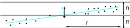
Note that ifκris large, even when there is no noise in the PCD, the normal to the best fit line may not be a good ap-proximation to the tangent as shown in Figure 1. Similarly, if σn/r is large and the noise is biased, this normal may
not be a good approximation even if the original curve is a straight line, see Figure 2. In order to keep the normal ap-proximation error low we assumea priorithatκrandσn/r
are sufficiently small.
r
κr2
Figure 1: Curvature causes error in the estimated normal
n n r
Figure 2: Noise causes error in the estimated normal
We assume that the data is evenly distributed; there is a radius r0 > 0 (possibly dependent on O) so that any
neighborhood of size r0 inR contains at least 2 points of
the xi’s but no more than some small constant number of
them. We observe that the number of points k inside any disk of radiusris bounded from above by Θ(1)rρ, and also is bounded from below by another Θ(1)rρ, where ρ is the sampling density of the point cloud. Here we use Θ(1) to denote some small positive constant, and for notational sim-plicity, different appearances of Θ(1) may denote different constants. We note that distributions satisfying the (, δ) sampling condition proposed by Dey et. al. [7] are evenly distributed.
Under the above assumptions, we would like to bound the normal estimation error and study the effects of different parameters. The analysis involves probabilistic arguments to account for the random nature of the noise.
2.2
Total Least Square Line
In this section, we briefly describe the well-known total least square method. Given a set of pointspi, 1≤i≤k,
we would like to find the lineaTx=c, withaTa= 1 such
that the sum of square distances from the points pi’s to
the line is minimized. Letf(a, c) = 1 2k k i=1(a Tp i−c)2 = 1 2a T 1 k k i=1pip T i a−cp¯ Ta+ 1 2c 2 where ¯p = 1 k k i=1pi.
We would like to findaandcminimizingf(a, c) under the constraint thataTa= 1.
To solve this quadratic optimization problem, we need to solve the following system of equations:
∂ ∂af(a, c) =λa ⇒ 1 k k i=1 pipTi a−cp¯=λa , ∂ ∂cf(a, c) = 0 ⇒ −p¯ Ta+c= 0,
where λ is a Lagrangian multiplier. It follows that c = ¯ pTa, 1 k k i=1pip T i −p¯p¯T a =λa, andf(a, c) = λ 2. Thus λ is an eigenvalue of M = 1 k k i=1pip T i −p¯p¯T with a as
the corresponding eigenvector. It is clear that to minimize
f(a, c), λ has to be the minimum eigenvalue of M. The corresponding eigenvectorais the normal to the total least square line and is our normal estimate.
Note that this approach can be generalized to higher di-mensional space. The normal to the total least square fit-ting plane (or hyperplane) of a set ofk pointspi,1≤i≤k
in d for d ≥ 2 can be obtained by computing the
eigen-vector corresponding to the smallest eigenvalue of M =
1 k
k i=1pip
T
i −p¯p¯T. We observe thatM can be written as
M= 1 k
k
i=1(pi−p¯)(pi−p¯)
T and thus it is always
symmet-ric positive semi-definite, and has non-negative eigenvalues and non-negative diagonal.
2.3
Eigen-analysis of
MWe can write the 2×2 symmetric matrix M, as defined in the previous section, as
m11 m12
m12 m22
. Note that in ab-sence of noise and curvature,m12 =m22= 0 which means
0 is the smallest eigenvalue ofM with [0 1]T as the corre-sponding eigenvector. Under our assumption that the noise and the curvature are small,yi’s are small, and thusm12and
m22are small. Letα= (|m12|+m22)/m11. We would like to
estimate the smallest eigenvalue ofM and its corresponding eigenvector whenαis small.
Using theGershgorin Circle Theorem[9], there is an eigen-valueλ1such that|m11−λ1| ≤ |m12|, and an eigenvalueλ2
such that|m22−λ2| ≤ |m12|. Whenα≤1/2, we have that
λ1 ≥m11− |m12| ≥m22+|m12| ≥λ2. It follows that the
two eigenvalues are distinct, and λ2 is the smallest
eigen-value ofM. Let [v1]T be the eigenvector corresponding to
λ2, then m11 m12 m12 m22 v 1 = λ2 v 1 , m11−λ2 m12 v = − m12 m22−λ2 . Thus v = −(m11−(λm2)m12+m12(m22−λ2) 11−λ2)2+m212 , (1) |v| ≤ |m12|(m11−λ2+|m12|) (m11−λ2)2 , ≤ α(1(1 +α) −α)2 .
Thus, the estimation error, which is the angle between the estimated normal and the true normal (which is [0 1]T in this
case), is less than tan−1
(α(1 +α)/(1−α)2
)≈α, for smallα. Note that we could write the error explicitly in closed form, then bound it. Our approach is more complicated, though as we will show later, it can be extended to obtain the error bound for the 3D case. To bound the estimation error, we need to estimateα.
2.4
Estimating Entries of
MThe assumption that the sample points are evenly dis-tributed in the interval [−r, r] implies that, given any num-ber x in that interval, the number of points pi’s
satisfy-ing |xi−x| ≥r/4 is at least Θ(1)k. It follows easily that
m11 = 1 k k i=1(xi−x¯) 2 ≥Θ(1)r2
. The constant Θ(1) de-pends only on the distribution of the random variableX.
For the entries m12 andm22, we use |xi| ≤rand |yi| ≤
κr2
/2 +nto obtain the following trivial bound:
|m12| = 1 k k i=1 xiyi− 1 k2 k i=1 xi k i=1 yi ≤ 2r(κr2/2 +n), m22 ≤ 1 k k i=1 y2 i ≤ 2((κr2/2)2+n2). Thus, α ≤ Θ(1) κr+n r +κ 2 r2+n 2 r2 ≤ Θ(1) κr+n r . (2)
This bound illustrates the effects of r, κ and n on the error. For large values ofr, the error caused by the curva-tureκrdominates, while for a small neighborhood the term
n/ris dominating. Nevertheless, the expression depends on the absolute bound n of the noise N. This boundn can be unnecessarily large or unbounded for many distribution models of N. We would like to use our assumption on the distribution of the noiseN to improve our bound onα fur-ther.
Note that |m12| = 1 k k i=1 xiyi− 1 k2 k i=1 xi k i=1 yi ≤ 1 k k i=1 (γix 3 i/2 +xini) + 1 k2 k i=1 xi k i=1 (γix 2 i/2 +ni) ≤ Θ(1)κr3+ 1 k k i=1 xini +Θ(1)r κr 2 + 1 k k i=1 ni .
Furthermore, under the assumption thatX andNare in-dependent, we haveE[xini] =E[xi]E[ni] = 0 sinceE[ni] =
0 and Var(xini) = Θ(1)r 2 σ2 n since Var(ni) = σ 2 n. Let
> 0 be some small constant. Using the Chebyshev In-equality[13], we can show that the following bound on|m12|
holds with probability at least 1−:
|m12| ≤ Θ(1)κr 3 + Θ(1) r 2σ2 n k + Θ(1)r σ2 n k = Θ(1)κr3 + Θ(1) r2σ2 n rρ + Θ(1)r σ2 n rρ ≤ Θ(1)κr3 + Θ(1)σn r ρ. (3)
For reasonable noise models, we also have that
m22 ≤ 1 k k i=1 2(γ2 ix 4 i/4 +n 2 i) ≤ Θ(1)κ2 r4 + Θ(1)σ2 n.
2.5
Error Bound for the Estimated Normal
From the estimations of the entries ofM, we obtain the following bound onα, with probability at least 1−:
α≤Θ(1)κr+ Θ(1) σn
ρr3 + Θ(1)
σ2 n
r2 . (4)
Note that this bound depends on the standard deviation
σnof the noiseN rather than its magnitude boundn.
For a given set of parametersκ,σn,ρ, and, we can find
the optimalrthat minimizes the right hand side of inequal-ity 4. As this optimal value ofr is not easily expressed in closed form, let us consider a few extreme cases.
• When there is no curvature (κ= 0) we can make the bound onαarbitrarily small by increasing r. For suf-ficiently large r, the bound is linear inσn and it
de-creases asr−3/2
.
• When there is no noise, we can make the error bound small by choosingras small as possible, sayr=r0.
• When both noise and curvature are present, the error bound cannot be arbitrarily reduced. When the den-sityρ of the PCD is sufficiently high,α ≤Θ(1)κr+
Θ(1)σ2 n/r
2
. The error bound is minimized whenr = Θ(1)σn2/3κ−
1/3
, in which case α≤Θ(1)κ2/3
σn2/3. The
sufficiently high density condition onρcan be shown to beρ >Θ(1)−1
σ−4/3 n κ−1/3.
• When there are both noise and curvature, and the den-sityρis sufficiently low,α≤Θ(1)κr+ Θ(1)σn/
ρr3.
The bound is smallest whenr = Θ(1)(σ2 n/(ρκ 2 ))1/5 , in which case, α ≤ Θ(1)(κ3 σ2 n/(ρ)) 1/5 . The suffi-ciently low condition onρcan be expressed more specif-ically as ρ < Θ(1)−1
σ−4/3
n κ−1/3. We would like to
point out that the constant hidden in the Θ(1) nota-tion in the “sufficiently low” condinota-tion is 3/4 of that in the “sufficiently high” condition.
3.
NORMAL ESTIMATION IN
3We can extend the results obtained for curves in 2
to surfaces in 3
. Given a point cloud obtained from a smooth 2-manifold in 3
and a pointO on the surface, we can esti-mate the normal to the surface atO as follows: find all the points of the PCD inside a sphere of radius r centered at
O, then compute the total least square plane fitting those points. The normal vector to the fitting plane is our esti-mate of the undirected normal atO.
Given a set ofkpointspi, 1≤i≤k, letM= 1 k k i=1pip T i− ¯ pp¯T, where ¯p= 1 k k
i=1pi. As pointed out in subsection 2.2,
the normal to the total least square plane for this set of
k points is the eigenvector corresponding to the minimum eigenvalue of the M. We would like to bound the angle between this eigenvector and the true normal to the surface.
3.1
Modeling
We model the PCD in a similar fashion as in the 2
case. We assume that O is the origin, the z-axis is the normal to the surface atO, and that the points of the PCD in the sphere of radiusraroundOare samples of a topological disk on the surface. Under these assumptions, we can represent the surface as the graph of a function z =g(x) where x = [x, y]T. Using Taylor Theorem, we can writeg(x) = 1
2x THx
where H is the Hessian of f at some point ψ such that |ψ| ≤ |x|.
We assume that the surface has bounded curvature in some neighborhood aroundO so that there is aκ >0 such that the Hessian H of g satisfies ||H||2 ≤κ in that
neigh-borhood.
Write the points pi as pi = (xi, yi, zi) = (xi, zi). We
assume thatzi=g(xi) +ni, where theni’s are independent
instances of some random variableN with zero mean and standard deviationσn. We similarly assume that the points
xiareevenly distributedin thexy-plane on a diskDof radius
r centered atO, i.e. there is a radiusr0 such that any disk
of sizer0 insideDcontains at least 3 points among thexi’s
but no more than some small constant number of them. We also assume that the noise and the surface curvature are both small.
3.2
Eigen-analysis in
3We write the analogous matrixM=
m11 m12 m13 m12 m22 m23 m13 m23 m33 = M11 M13 MT 13 m33
sym-metric and positive semi-definite. Under the assumptions that the noise and the curvature are small, and that the points xi are evenly distributed, m11and m22 are the two
dominant entries inM. We assume, without lost of general-ity, thatm11≤m22. Letα= (|m13|+|m23|+m33)/(m11−
|m12|). As in the 2
case, we would like to bound the angle between the computed normal and the true normal to the point cloud in term ofα.
Denote byλ1≤λ2the eigenvalues of the 2×2 symmetric
matrixM11. Using again the Gershgorin Circle Theorem, it
is easy to see thatm11− |m12| ≤λ1, λ2≤m22+|m12|.
Letλbe the smallest eigenvalue of M. From the Gersh-gorin Circle Theorem we haveλ≤ |m13|+|m23|+m33 =
α(m11−m12)≤αλ1. Let [vT 1]T be the eigenvector of M
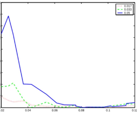
corresponding with λ. Then, as with Equation 1, we have that: v = − (M11−λI) 2 +M13M13T −1 ((M11−λI)M13+M13(m33−λ)) = −(M11−λI)− 2 I+ (M11−λI)− 2 M13M13T −1 ((M11−λI)M13+M13(m33−λ)), ||v||2 ≤ ||(M11−λI)− 2 ||2× I+ (M11−λI)− 2 M13M13T −1 2 × (||(M11−λI)||2||M13||2+||M13||2|m33−λ|). Note that ||(M11−λI)− 2 M13M13T||2 ≤ ||(M11−λI)− 2 ||2||M13||2||M13T||2 ≤(λ1−λ)− 2 (m2 13+m 2 23) ≤(1−α)−2 α2 . Thus I+ (M11−λI)− 2 M13M13T −1 2 ≤1 1 −(1−α)−2α2 ≤ (1−α)2 1−2α . It follows that ||v||2 ≤ 1 (1−α)2λ2 1 (1−α)2 1−2α (λ2αλ1+αλ1αλ1) ≤ α1(1 +α) −2α λ2 λ1 .
When α is small, the right hand side is approximately (λ2/λ1)α, and thus the angle between the computed normal
and the true normal, tan−1
||v||2, is approximately bounded
by (λ2/λ1)α≤((m22+|m12|)/(m11− |m12|))α,
3.3
Estimation of the entries of
MAs in the 2
case, from the assumption that the sam-ples are evenly distributed, we can show that Θ(1)r2
≤
m11, m22 ≤r 2
. We can also show that m33 ≤Θ(1)κ 2
r4
+ Θ(1)σ2
n. Let ρbe the sampling density of the PCD at O,
then k = Θ(1)ρr2
. Again, let >0 be some small posi-tive number. Using the Chebyshev inequality, we can show that m13, m23 ≤ Θ(1)κr 3 + Θ(1)σnr/ √ k ≤ Θ(1)κr3 + Θ(1)σn/√ρwith probability at least 1−. For the term
m12, we note thatE[xiyi] = 0 andV ar(xiyi) = Θ(1)r4, and
so, by the Chebyshev inequality, m12 ≤ Θ(1)r/√ρ with
probability at least 1−.
3.4
Error Bound for the Estimated Normal
Letβ =m12/m11. We restrict our analysis to the cases
whenβis sufficiently less than 1, sayβ <1/2. This restric-tion simply means that the points xi’s are not degenerate, i.e. not all of the points xi’s are lying on or near any given line on thexy-plane. With this restriction, it is clear that (λ2/λ1)α≤(m22/m11)((1 +β)/(1−β))α= Θ(1)α.
From the estimations of the entries ofM, we obtain the following bound with probability at least 1−:
λ2 λ1 α ≤ Θ(1)κr+ Θ(1) σn r2√ρ Θ(1)κ2 r2 + Θ(1)σ 2 n r2 ≤ Θ(1)κr+ Θ(1) σn r2√ρ+ Θ(1) σ2 n r2
This is an approximate bound on the angle between the estimated normal and the true normal. To minimize this error bound, it is clear that we should pick
r= 1 κ c1 σn √ρ+c2σ 2 n 1/3 , (5)
for some constantsc1,c2. The constantsc1andc2 are small
and they depend only on the distribution of the PCD. We notice that from the above result, when there is no noise, we should pick the radiusrto be as small as possible, sayr=r0. When there is no curvature, the radiusrshould
be as large as possible. When the sampling density is high, the optimal value of r that minimizes the error bound is approximately r= Θ(1)(σ2
n/κ) 1/3
. This result is similar to that for curves in 2
, and it is not at all intuitive.
4.
EXPERIMENTS
In this section, we discuss some simulations to validate our theoretical results. We then show how to use the re-sults in obtaining a good neighborhood size for the normal computation with the least square method.
4.1
Validation
We considered a PCD whose points were noisy samples of the curves (x, κsgn(x)x2
/2), forx∈[−1,1] for different values ofκ. We estimated the normals to the curves at the origin by applying the least square method on their corre-sponding PCD. As they-axis is known to be the true normal to the curves, the angles between the computed normals and they-axis gives the estimation errors.
To obtain the PCD in our experiments, we let the sam-pling density ρ be 100 points per unit length, and let x
be uniformly distributed in the interval [−1,1]. The y -components of the data were polluted with uniformly ran-dom noise in the interval [−n, n], for some value n. The standard deviationσnof this noise isn/
√ 3.
Figure 3 shows the error as a function of the neighborhood sizerwhenn= 0.05 for 3 different values ofκ,κ= 0.4,0.8, and 1.2. As predicted by Equation 4 for large value ofr, the error increases asrincreases. In the experiments, it can be seen that the error is proportional toκr for r >0.2. Note
that the PCD we chose generates the worst case behavior of the error. 0 0.1 0.2 0.3 0.4 0.5 0.6 0.7 0.8 0.9 1 0 0.2 0.4 0.6 0.8 1 1.2 Radius Error Angle 0.4 0.8 1.2
Figure 3: The normal estimation error increases as
r increases forr >0.2.
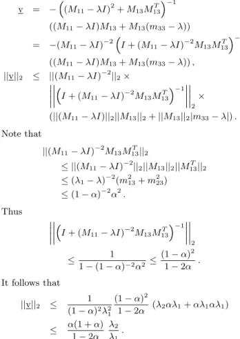
Figure 4 shows the estimation error as a function of the neighborhood sizerfor smallrwhenκ= 1.2 for 3 different values ofn,n= 0.017,0.033, and 0.05. We observe that the error tends to decrease asr increases forr <0.08. This is expected as from Equation 4, the bound on the error is a decreasing function ofr whenris small.
0.020 0.04 0.06 0.08 0.1 0.12 0.2 0.4 0.6 0.8 1 1.2 1.4 1.6 1.8 0.017 0.033 0.05 Radius Error Angle
Figure 4: The normal estimation error decreases as
ndecreases and r increases for r <0.08.
The dependency of the error onrfor small values ofrcan be seen more easily in Figure 5, which shows the average of the estimation errors over 50 runs for eachr.
4.2
Estimating Neighborhood Size for the
Nor-mal Computation
In this part, we used the results obtained in Section 3 to estimate the normals of a PCD. The data points in the PCD were assumed to be noisy samples of a smooth surface in 3
. This is the case, for example, for PCD obtained by range scanners. To obtain the neighborhood size for the normal computation using the least square method, we would like to use Equation 5.
We assumed that the standard deviationσn of the noise
was given to us as part of the input. We estimated the other local parameters in Equation 5, then computedr. Note that this value ofrminimizes the bound of the normal computa-tion error, and there is no guarantee that this would mini-mize the error itself. The constantsc1andc2depend on the
0.020 0.04 0.06 0.08 0.1 0.12 0.1 0.2 0.3 0.4 0.5 0.6 0.7 0.8 0.9 Radius Error Angle 0.017 0.033 0.05
Figure 5: The average error over 50runs exhibits a clear tendency to decrease asr increases for smallr.
Figure 6: Tangent planes on the original bunny
sampling distribution of the PCD. While we could attempt to compute the exact values ofc1andc2, we simply guessed
the valuec1 andc2. The value ofwas fixed at 0.1.
Given a PCD, we estimated the local sampling density as follows. For a given point p in the PCD, we used the approximate nearest neighbor library ANN [5] to find the distancesfrompto itsk-th nearest neighbor for some small numberk,k = 15 in our experiments. The local sampling density atpwas then approximated asρ=k/(πs2
) samples per unit area.
To estimate the local curvature, we used the method pro-posed by Gumhold et al. [10]. Letpj, 1≤j≤k be thek
nearest sample points around p, and letµ be the average distance frompto all the pointspj. We computed the best
fit least square plane for those k points, and let d be the distance from pto that best fit plane. The local curvature atpcan then be estimated asκ= 2d/µ2
.
Once all the parameters were obtained, we computed the neighborhood size r using Equation 5. Note that the esti-mated value ofrcould be used to obtain a good value fork, which can to be used to re-estimate the local density and the local curvature. This suggests an iterative scheme in which we repeatedly estimate the local density, the local curva-ture, and the neighborhood size. In our experiments, we found that 3 iterations were enough to obtain good values for all the quantities.
We still have problems with obtaining good estimates for the constantsc1 andc2. Fortunately, we only have to
esti-mate the constants once for a given PCD, and we can use the same constants for many PCD with a similar point dis-tribution. In our experiments, we used the same value for both c1 and c2. This value was chosen so that the
com-puted normals on a small region of the PCD were visually satisfactory.
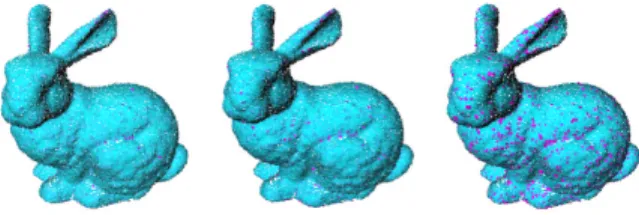
orig-Figure 7: Normal estimation errors for the bunny PCD with noise added. The subfigures show the points of the PCD using the pink color whenever the errors are above10◦,8◦,and 5◦ respectively.
inal Stanford bunny. The planes are drawn as small fixed size square patches1
. We noted that our computed normals are similar to those obtained using thecocone method by Amenta et al. [4].
Noisy PCD used in our experiments were obtained by adding noise to the original bunny. Thex,y, andz compo-nents of the noise were chosen independently and uniformly random in the range [−0.0005,0.0005]. The amplitude of this noise is comparable to the average distance between the sample points and their nearest samples.
We computed the normals of the noisy PCD, and used the angles between those normals and the normals of the origi-nal PCD as estimates of the normal computation errors. In Figure 7, we color coded the estimation errors using a con-vention in which the color of the square patch at a point of the PCD showed the error at that point. The color of a patch is blue when there is no error, and it gets darker as the error increases. When the error is larger than a certain threshold, the patch becomes pink. Figure 7 shows the tangent planes where the thresholds are 10◦, 8◦, and 5◦respectively.
We ran the least square normal estimation algorithm on the bunny with different amounts of noise added to it and observed that the algorithm worked well. We also noted that the normal estimation method based on cocone performed poorly in the presence of noise.
5.
CONCLUSIONS
We have analyzed the method of least square in estimating the normals to a point cloud data derived either from a smooth curve in 2
or a smooth surface in 3
, with noise added. In both cases, we provided theoretical bound on the maximum angle between the estimated normal and the true normal of the underlying manifold. This theoretical study allowed us to find an optimal neighborhood size to be used in the least square method.
6.
ACKNOWLEDGMENTS
We would like to thank Leonidas Guibas for his sugges-tions, comments and encouragement. We are grateful to Tamal K. Dey for useful discussions and also for providing the software for evaluating normals usingcocone. We also thank Marc Levoy, Ron Fedkiw for helpful discussions. We acknowledge the generous support of the Stanford Graduate Fellowship program and of NSF CARGO grant 0138456.
1
The small holes in the bunny are observable due to the fact that the patches do not cover the bunny entirely.
We also want to thank the numerous referees of the pre-vious versions of this paper for their extremely useful sug-gestions.
7.
REFERENCES
[1] M. Alexa, J. Behr, D. Cohen-Or, S. Fleishman, D. Levin, and C. T. Silva. Point set surfaces. IEEE Visualization 2001, pages 21–28, October 2001. ISBN 0-7803-7200-x.
[2] N. Amenta, M. Bern, and M. Kamvysselis. A new Voronoi-based surface reconstruction algorithm.
Computer Graphics, 32(Annual Conference Series):415–421, 1998.
[3] N. Amenta and M. W. Bern. Surface reconstruction by voronoi filtering. InSymposium on Computational Geometry, pages 39–48, 1998.
[4] N. Amenta, S. Choi, T. K. Dey, and N. Leekha. A simple algorithm for homeomorphic surface reconstruction.International Journal of Computational Geometry and Applications, 12(1-2):125–141, 2002.
[5] S. Arya, D. M. Mount, N. S. Netanyahu,
R. Silverman, and A. Y. Wu. An optimal algorithm for approximate nearest neighbor searching fixed dimensions.Journal of the ACM, 45(6):891–923, 1998. [6] J.-D. Boissonnat and F. Cazals. Smooth surface
reconstruction via natural neighbour interpolation of distance functions. InSymposium on Computational Geometry, pages 223–232, 2000.
[7] T. K. Dey, J. Giesen, S. Goswami, and W. Zhao. Shape dimension and approximation from samples. In
Proc. 13thACM-SIAM Sympos, Discrete Algorithms,
pages 772–780, 2002.
[8] S. Funke and E. Ramos. Smooth-surface reconstruction in near-linear time, 2002.
[9] G. Golub and C. V. Loan.Matrix Computations. The John Hopkins University Press, Baltimore, 1996. [10] S. Gumhold, X. Wang, and R. MacLeod. Feature
extraction from point clouds. In 10th International Meshing Roundtable, Sandia National Laboratories, pages 293–305, October 2001.
[11] H. Hoppe, T. DeRose, T. Duchamp, J. McDonald, and W. Stuetzle. Surface reconstruction from unorganized points.Computer Graphics, 26(2):71–78, 1992. [12] I. Lee. Curve reconstruction from unorganized points.
Computer Aided Geometric Design, 17:161–177, 2000. [13] A. Leon-Garcia. Probability and Random Processes for
Electrical Engineering. Addison Wesley, 1994. [14] S. Rusinkiewicz and M. Levoy. QSplat: A
multiresolution point rendering system for large meshes. In K. Akeley, editor,Siggraph 2000, Computer Graphics Proceedings, pages 343–352. ACM Press / ACM SIGGRAPH / Addison Wesley Longman, 2000. [15] W. Welch and A. Witkin. Free-form shape design
using triangulated surfaces. Computer Graphics, 28(Annual Conference Series):247–256, 1994. [16] M. Zwicker, M. Pauly, O. Knoll, and M. Gross.
Pointshop 3d: An interactive system for point-based surface editing. InProc. ACM SIGGRAPH ’02, Computer Graphics Proceedings, Annual Conference Series, 2002.