Variable selection
in partially linear wavelet models
H. Ding and G. Claeskens
DEPARTMENT OF DECISION SCIENCES AND INFORMATION MANAGEMENT (KBI)
Faculty of Business and Economics
Variable Selection in Partially Linear
Wavelet Models
Huijuan Ding and Gerda Claeskens
K.U. Leuven
ORSTAT and Leuven Statistics Research Center
Naamsestraat 69, 3000 Leuven, Belgium
[email protected]; [email protected]
December 3, 2008
Abstract
Variable selection is fundamental in high-dimensional statistical modeling, including non- and semiparametric regression. However little work has been done for variable selection in a partially linear model. We propose and study a unified approach via double penalized least squares, retaining good features of both variable selection and model estimation in the framework of partially linear models. The proposed method is distinguished from others in that the penalty functions combine the`1 penalty coming
from wavelet thresholding in the nonparametric component with the `1 penalty from the lasso in the parametric component. Simulations are used to investigate the per-formance of the proposed estimator in various settings, illustrating its effectiveness for simultaneous variable selection as well as estimation.
Keywords: Lasso, `1 penalty, Partially linear model, Variable selection, Wavelet estimation.
1
Introduction
We propose and study a unified approach for simultaneous variable selection and model estimation in partially linear models. Consider the following regression model:
Yi =xtiβ+f(ti) +εi, i= 1,2, . . . , N (1)
where {Yi} is the response variable, {xi} are known design points and each is a fixed p
-dimensional vector with corresponding parameter vector β of lengthp, {ti} are values of an
extra univariate variable such as, for example, the time at which the observation is made,f(·) is an unknown function that is potentially non-smooth, εi are random errors assumed to be
independent and identically distributed as N(0, σ2). Without loss of generality, we assume
t ∈ [0,1]. The goal is to estimate both the nonparametric function f(·) and the parameter vector β. Our estimation method will allow for the selection of important variables in the parametric part of the model by using a `1 lasso penalty on the regression coefficients. For the nonparametric part we use wavelet estimators which allow the true function to be non-smooth.
The partially linear model (PLM) in (1), with parametric componentxTβ and
nonpara-metric component f(t), enjoys the flexibility of the nonparametric models, while maintain-ing the easy interpretation of parametric models. Various estimation procedures and their asymptotic properties have been established by Heckman (1986), Rice (1986), Speckman (1988), Hamilton and Truong (1997), amongst others. For more details and references, see H¨ardle et al. (2000).
In this paper, we use the wavelet nonparametric regression procedure for the PLM. The main reason for adopting wavelets is to avoid the smoothness assumption on f(·), that is used by most of the existing approaches such as kernel, local polynomial or spline estimators. Wavelet smoothing makes less restrictive assumptions about the smoothness of the underlying function, allowing for possible sharp transitions, jumps, and sharp peaks. At
the same time, wavelets lead to a sparse representation that can be easily compressed or denoised using thresholds for wavelet coefficients, see Donoho and Johnstone (1994), and Donoho et al. (1995).
Chang and Qu (2004) proposed a wavelet-soft thresholding estimator for the PLM and developed an efficient descent algorithm with an exact line search. A regularized estimator was introduced by Fadili and Bullmore (2004), which can be efficiently estimated by choosing an appropriate penalty function for which the hard and soft thresholding estimators are particular cases. Fadili (2005) extended modeling the nonparametric component in PLMs from orthogonal bases (complete) to redundant (overcomplete) expansions in the wavelet domain. For the estimation of the nonparametric part of the PLM, we will apply an iterative backfitting-like algorithm as well as soft thresholding.
The main novel part of this paper is the inclusion of variable selection for the parametric part of the model. Identifying significant predictors will enhance the prediction performance of the fitted model. While there is a vast amount of work on variable selection for linear models, little work has been done for variable selection in partially linear models, however, see Simonoff and Tsai (1999), and Li and Liang (2008) for methods using local likelihood estimators for the nonparametric part of the model. The lasso, short for “least absolute shrinkage and selection operator”, proposed by Tibshirani (1996), achieves the goal of si-multaneous estimation and variable selection by introducing an `1 penalty on the regression coefficients in linear models. The resulting lasso estimate of β can contain some exact zero coefficients, which is equivalent to excluding the corresponding variables from the final model. Theoretical properties of the lasso estimator have been obtained by Knight and Fu (2000) and Zhao and Yu (2006), amongst others. Zou (2006) proposed the adaptive lasso in which adaptive weights are used for penalizing different coefficients in the `1 penalty.
In this paper, we use the adaptive lasso to select relevant variables in parametric com-ponent of the model. Together with the soft-thresholded wavelet estimation method for
the nonparametric part of the model, this leads to a double penalized estimator, using `1 penalties for both model parts.
The rest of the paper is organized as follows. In Section 2, we introduce our new double-penalty estimation procedure for partially linear models. Section 3 contains details about the practical implementation using an iterative algorithm, which iterates between fitting a nonparametric wavelet regression model and minimizing a penalized least squares objective function. In Section 4 we discuss how to adaptively select the tuning parameters. A simple yet effective stagewise tuning procedure is presented. Monte Carlo studies and an application involving real data are shown in Section 5. Some discussion is given in Section 6.
2
A double penalized estimation method
We introduce our estimation method where the penalty functions combine an `1 penalty coming from wavelet thresholding in the nonparametric part (see Section 2.1) with a second
`1 penalty from the adaptive lasso in the parametric part (see Section 2.2). Thus we achieve simultaneously the objectives of variable selection and model estimation in the partially linear model.
2.1
Wavelet smoothing in the partially linear model
We are working with a wavelet basis that is generated through a mother wavelet functionψ(·) and father scaling function φ(·). Defining the normalized functions ψjk(t) = 2j/2ψ(2jt−k)
and φjk(t) = 2j/2φ(2jt−k) for j ≥j0 = 0 (the resolution level) and k = 0, . . . ,2j −1, gives an orthonormal basis ofL2[0,1], the square integrable functions on [0,1]. The nonparametric part of the PLM (1) can then be represented by the wavelet series expansion
f(t) = 2Xj0−1 k=0 cj0,kφj0,k(t) + J−1 X j=j0 2j−1 X k=0 γj,kψj,k(t), (2)
where the sample size N = 2J. In practice, the coefficients in this expansion follow from a
discrete wavelet transformation (DWT), leading to empirical scale and wavelet coefficients ˆ
cj0,k and ˆγj,k. Denoting W
t the inverse DWT matrix containing the scaling and wavelet
functions in its columns, which has dimensionN×N andδ = (c,γ) the vector of all scaling and wavelet coefficients, the PLM in (1) can be written in matrix form as
Y =Xβ+Wtδ+ε.
For identifiability, we here consider that the vector 1N is not spanned by the vectors of X,
i.e., the mean of the vector Y is explained by Wtδ.
Wavelet estimation has the important advantage of creating a sparse signal, meaning that most of the wavelet coefficients are zero or close to zero, while important features of the signal are captured by large wavelet coefficients. This allows thresholding procedures to be used. Hard thresholding removes small wavelet coefficients and leaves other coefficients untouched. In contrast, soft thresholding works as a shrinkage method that shrinks large wavelet coefficients towards zero by the threshold value, and removes the small ones that do not exceed the threshold. A particular aspect of this method is that soft thresholding corresponds to placing an `1 penalty on the wavelet coefficients, while leaving the scaling coefficients unpenalized. In detail, this leads to the first penalty term in the objective function of the double penalized estimation method (3) where λ1 is the threshold value.
2.2
Lasso as a variable selection method
The lasso method as proposed by Tibshirani (1996) for linear regression models of the type
Y =Xβ+ε, puts a `1 penalty on the regression coefficients. The lasso estimator ˆβ is the minimizer over β of the penalized least squares criterion
kY −Xβk2+λ 2 p X j=2 |βj|,
where p denotes the number of regression variables. Note that the intercept, which is in the parametric model included in the design matrix X, is not bounded by the constraint. A particular useful aspect of the properties of an `1 penalty is that it not only shrinks the coefficients towards zero, but also allows some of the coefficients to be identically zero. This aspect makes that the lasso can be used as a variable selection method.
While the lasso applies the same penalty to all of the regression coefficients, the adaptive lasso (Zou, 2006) has different weights τj for each coefficient. This leads to a minimization
problem of a penalized least squares criterion of the form
kY −Xβk2+λ 2 p X j=2 τj|βj|.
As a result, large amounts of shrinkage can be used for insignificant variables, while small amounts of shrinkage can be used for significant variables. Zou (2006) showed that for certain data-dependent values for the weightsτi, the adaptive lasso has oracle properties in the sense
of performing equally well as if the true model were known.
2.3
The double penalty estimation approach
We propose to minimize the following double penalized least-squares criterion to estimateβ
and γ: min β∈Rp,δ∈RNl(β,δ) =β∈Rminp,γ∈RN © kY −Xβ−Wtδk2+λ1 J−1 X j=j0 2j−1 X k=0 |γj,k|+λ2 p X i=1 τi|βi| ª . (3)
The threshold valueλ1 controls the sparsity of nonparametric estimates, while for the purpose of variable selection we impose the weighted `1 penalty on the linear coefficientsβ and thus use λ2 to control the sparsity of the parametric part of the model. We will give more details about the choice of the regularization parameters λ1 and λ2 in Section 4.
An iterative algorithm will be used to solve the above estimation problem (3) with any fixed λ1 and λ2. The main idea is to successively minimize the objective function l(β,γ)
with respect to β while holding γ fixed, and next minimize l(β,γ) with respect to γ while holding β fixed. All the computational details are presented in Section 3.
Before minimizing the objective function (3), the adaptive weights τi should be defined.
We propose to take ˆτ = 1/|β˜|, where ˜β is the estimate for β in the PLM model (1) without putting a penalty on the parametric part of the model. To obtain our initial estimators ( ˜β,γ˜) that are used in the iterative procedure as well as in the weights of the adaptive lasso, we apply the wavelet estimation method for the partially linear model by Fadili and Bullmore (2004) and Fadili (2005), which only includes an `1 penalty on the wavelet coefficients and leaves all other coefficients unpenalized. Using the orthogonality of the DWT matrix W, the initial estimators are obtained by minimizing over (β,δ), the penalized function
kW Y −W Xβ−δk2+λ J−1 X j=j0 2j−1 X k=0 |γj,k|,
where the penalty takes action only on the wavelet coefficients, not on the scaling coefficients, nor on the coefficients of the parametric part of the model.
The idea of double-penalized least squares has been used in other contexts. Tibshirani and Saunders (2005) proposed the ‘fused lasso’, which penalizes the `1 norm of both the coefficients and their successive differences. This corresponds to expressing sparsity in the coefficients as well as in their differences. Wang et al. (2007) also used double `1 penalties for a linear regression model with autoregressive errors. One penalty is for the regression coefficients, the other for the autoregression coefficients. Our double-penalized least squares criterion in the partially linear model is new. The penalty functions combine the `1 penalty coming from wavelet thresholding in the nonparametric part with the `1 penalty from the adaptive lasso in the parametric part. Thus we achieve the objectives of variable selection and model estimation simultaneously.
3
Algorithm
Now we propose an iterative algorithm to minimize the double penalized least squares cri-terion function (3) for any fixed choice of regularization parameters λ1 and λ2. We use a backfitting type of algorithm which iterates between minimizing the following adaptive lasso-type criterion ( β-step) and a wavelet-type objective function (δ-step):
β-step : min β {kY −Xβ−W tδk2+λ 2 p X i=1 τi|βi|} with a fixed δ (4) δ-step : min δ {kY −Xβ−W tδk2+λ 1 J−1 X j=j0 2j−1 X k=0 |γj,k|} with a fixed β. (5)
In a similar spirit, Wang et al. (2007) used such an algorithm for their double `1 penalty approach.
To obtain the initial estimators, according to Theorem 1 of Fadili and Bullmore (2004), the backfitting algorithm can be used to estimate the parametric and the non-parametric part of the PLM, including soft thresholding for the wavelet estimator.
Algorithm 1. The (single) penalized PLM wavelet estimator
1. Calculate the columnwise DWT of Y and X. Set l = 0, γ(0)= 0. 2. For l= 0,1,2, . . . until convergence
(a) β(l+1) = (XtX)−1XtWt(W Y−δ(l)), i.e. least squares fit onW Y −δ(l).
(b) Wavelet fit on Y −Xβ(l+1), no penalty on the scaling coefficients and soft-thresholding for the wavelet coefficients, leading to
c(jl0+1),k = (W Y −W Xβ(l+1))k if k <2j0 + 1
γj,k(l+1) = sgn(rj,k(l+1)) max{|rj,k(l+1)| −λ,0},
For the adaptive, or weighted lasso, several well developed procedures can be used to find the minimizers of the lasso-type (β-step) problem. Examples include quadratic programming (Tibshirani, 1996), the shooting algorithm (Fu, 1998), a local quadratic approximation (Fan and Li, 2001), and more recently the least angle regression method (Efron et al., 2004). The shooting algorithm for the lasso was developed based on the theoretical results of the structure of the bridge estimators by (Fu, 1998). Particularly, it has a simple closed form and leads to fast convergence. These properties make it computationally attractive. We will use the slightly modified shooting algorithm, see Zhang and Lu (2007). The wavelet-type problem (δ-step), withβ fixed at its current value is a standard wavelet smoothing problem, and the solution is a soft-thresholding rule, which is in line with the solution for the non-parametric part of the PLM model. The algorithm is presented below.
Algorithm 2. The double penalized PLM wavelet estimator
1. Obtain the single penalized PLM wavelet estimator, denote the solution as (β,˜ δ˜). Set β(0) =β˜, δ(0) =δ˜.
2. Let k =k + 1. Minimize (4) with respect to β with δ(k−1) fixed at its current value. Denote the solution byβ(k).
3. Minimize (5) with respect to δ with β(k) fixed at its current value. Denote the solution byδ(k).
4. Go to step 2 until convergence.
In practice, only a small number of iterations is usually needed to achieve convergence. This is partially due to the fact that the penalized PLM wavelet estimator resulting from application of algorithm 1, can provide a good initial estimate.
4
Choice of regularization parameters
To implement the methods described in the previous sections, it is desirable to obtain the tuning parameters λ1 and λ2 in a data-driven way. To choose the regularization parameters (λ1, λ2) jointly by minimizing some performance criterion is computationally expensive in practice, since it involves a two-dimensional search. We propose a two-stage tuning pro-cedure. We first select λ1 at step 1 of the computational algorithm by GCV and at the successive steps, we fix the choice of λ1. We select the data-driven λ2 value through a grid search method. At each grid value of λ2, when the algorithm has converged, we re-calculate the optimal λ1 based on the converged estimate of the parametric parameters β. Then we select λ2 through a model fit criterion (see below).
There are several approaches in the literature for the choice of the λ1 in the context of wavelet regression. These methods include the traditional universal threshold value λ =
σ√2logN, Stein’s unbiased risk estimator SURE (Donoho and Johnstone, 1995) and cross validation (Nason, 1996). The threshold can easily be made level-dependent in case of correlated noise or non-orthogonal transforms, provided that all levels are sufficiently sparse for accurate estimation of the level-dependent standard deviation. The threshold adopted here is the generalized cross validation (GCV), see Jansen et al. (1997).
Various criteria have been proposed for the choice ofλ2. The well-known criteria include Mallow’sCp (1973), AIC (Akaike, 1973), BIC (Schwarz, 1978), cross-validation (CV) and the
generalized cross-validation (GCV) as suggested by Tibshirani (1996) for the lasso. While the AIC has the efficiency property, BIC is consistent in the sense that it almost surely identifies the true sparse model provided that the true model is in the candidate list. Due to the overfitting property of AIC, which is a known result in linear regression, AIC lasso shrinkage might include more non-zero predictors than necessary. For that reason Zou et al. (2007) suggested using BIC as the model selection criterion when the sparsity of the model
is of primary concern. They proposed BIC for the lasso as BIC(λ2) = kY −Xβˆ−fˆk nσ2 + log(N) N dfˆ(λ2)
where df(λ2) stands for the degree of freedom of the lasso, which is the number of nonzero coefficients of ˆβ. In the semiparametric regression models, we use the consistent estimate for the residual variance, i.e., ˆσ2 = 1/NPN
i=1εˆ2i, and ˆεi =yi−xTi βˆ−fˆ(ti), see Cheng (2005).
By the connection between AIC and BIC, the AIC is equivalently defined as AIC(λ2) =
kY −Xβˆ−fˆk
Nσ2 +
2
Ndfˆ(λ2).
To select the parameter λ2, we can also use the generalized cross-validation (GCV) method Craven and Wahba (1979), as suggested by Fu (1998) for the lasso model,
GCV = RSS
N(1−p(λ)/N)2
where p(λ) is the effective number of parameters of the model and it can be computed as
p(λ) = trace(X(XtX +λZ−)−1Xt)−n
0
whereZ− is the generalized inverse ofZ = diag(2|β| · |ˆ β|˜), and it has an extra compensation
term n0, i.e., the number of zero coefficients as compared to the one in Tibshirani (1996). We compare the three methods in a simulation study.
5
Numerical studies
In this section we summarize our simulation studies carried out to evaluate the finite-sample performance of the lasso and adaptive lasso estimators via the proposed double penalized least square procedure. For comparison purposes, the performance of the lasso and adaptive lasso estimators based on BIC, AIC and GCV criteria are evaluated in terms of mean squared error (MSE). We also include the “oracle model” fit, which is given by the single penalized PLM wavelet estimator when assuming that the true model is known. The oracle results are used for easy comparison but they are generally not available for real data.
5.1
Simulation models
We generated data from the semiparametric model Yi =xtiβ+f(ti) +εi, whereε∼N(0, σ2)
with σ = 1. Specifically, we set p = 20, and β = (1.5,2,2.5,3,0, . . . ,0)t. In other words,
the first 4 regression variables are significant, but the rest are not. In addition, the covariate vectors (X1, . . . , X20)t were independently generated from the 20-dimensional multivariate normal distribution with mean 020×1, variance 1, and the pairwise correlation coefficient is chosen to be ρ= 0.4. We generate the nonparametric component in two different cases, see Figure 1.
• Case I. f1 given in Nason (1996), is a piecewise polynomial with discontinuity;
f1(t) = 4t2(3−4t) if 0≤t≤0.5 4 3t(4t2 −10t+ 7)−1.5 if 0.5< t≤0.75 16 3 t(t−1)2 if 0.75< t≤1
• Case II. f2 given in Donoho and Johnstone (1994), is a function with many bumps.
f2(t) = ‘Bumps’.
For the DWT, we used the Daubechies filter with 8 vanishing moments. We choose
f(t) = 9f1 and f(t) = 3f2 in different settings to have a reasonable signal-to-noise ratios of the nonparametric and parametric component. The sample sizes used are N = 128 and 256. We use the proposed algorithm to estimate the true β. In our algorithm, the GCV was used to choose λ1 and λ2 was chosen by BIC, AIC and GCV respectively. We will compare the performance of traditional lasso and the adaptive lasso (Alasso) based on different smoothing parameter selection criteria in the simulation study.
0 0.5 1 0 0.2 0.4 0.6 0.8 1 f 1 0 0.5 1 0 1 2 3 4 f 2
Figure 1: Plot of the nonparametric functionsf1(t), which is piecewise polynomial, andf2(t),
the bumps function.
5.2
Performance of semiparametric estimators
5.2.1 Performance of ˆβWe assess the performance of an underlying parametric estimator βˆ via its mean squared error (MSE), Ekβˆ−βk2. To evaluate the MSE, we conducted K replicates of Monte Carlo simulations and the MSE is estimated by
1 K K X k=1 kβˆk−βk2.
In our simulations, K = 1000. The results are summarized in Tables 1 and 2 for both cases I and II.
As concerns the selection of predictors, four scenarios can occur. The best scenario would be to select exactly the set of 4 relevant predictors, namely correctly fitted. Another possi-bility is underfitted, i.e., all selected predictors are relevant, but not all relevant predictors are selected. Overfitting means that all relevant predictors are selected as well as some re-dundant predictors. The remaining scenario is the selection of a model including some, but not all, relevant and some redundant predictors. The last scenario does not occur in our
T able 1: Sim ulation results for f ( t ) = 9 f1 ( t ). The table sho ws for the sim ulation the p ercen tage of correctly selected variables, of ov erfit and of underfit mo dels in the parametric part of the PLM; as w ell as mean, standard deviation (SD) of parameter estimators, the MSE and av erage num b er of zeros selected, divided in to correct and incorrect selections of zeros. Sample size n = 128 n = 256 Estimator Lasso Adaptiv e Lasso Oracle Lasso Adaptiv e Lasso Oracle T uning Metho d BIC AIC GCV BIC AIC GCV BIC AIC GCV BIC AIC GCV underfit 0.017 0.013 0.000 0.006 0.006 0.000 0 0.002 0.002 0.000 0.000 0.000 0.000 0 Regression correct 0.554 0.462 0.020 0.753 0.660 0.017 1 0.528 0.418 0.000 0.782 0.676 0.002 1 V ariables ov erfit 0.429 0.525 0.981 0.241 0.334 0.983 0 0.470 0.580 1.000 0.218 0.324 0.998 0 ˆβ1 1.218 1.245 1.431 1.286 1.298 1.493 1.502 1.336 1.353 1.476 1.341 1.353 1.498 1.501 SD (0.299) (0.288) (0.128) (0.279) (0.282) (0.126) (0.123) (0.184) (0.188) (0.083) (0.198) (0.199) (0.082) (0.081) ˆβ2 1.813 1.830 1.952 1.926 1.930 1.993 1.994 1.897 1.908 1.985 1.955 1.959 2.000 2.001 SD (0.274) (0.260) (0.143) (0.215) (0.213) (0.143) (0.139) (0.155) (0.155) (0.092) (0.122) (0.121) (0.092) (0.090) Mean ˆβ3 2.331 2.346 2.467 2.421 2.425 2.501 2.506 2.402 2.412 2.487 2.437 2.442 2.500 2.500 SD (0.247) (0.243) (0.139) (0.184) (0.184) (0.140) (0.138) (0.134) (0.135) (0.089) (0.120) (0.119) (0.090) (0.087) ˆβ4 2.703 2.731 2.921 2.909 2.914 2.995 2.997 2.832 2.850 2.974 2.936 2.941 2.999 2.999 SD (0.342) (0.322) (0.131) (0.189) (0.190) (0.129) (0.122) (0.195) (0.198) (0.086) (0.112) (0.113) (0.085) (0.079) MSE ˆβ 0.573 0.503 0.088 0.259 0.253 0.072 0.068 0.189 0.177 0.032 0.116 0.111 0.030 0.028 Av e. zeros 14.736 14.060 9.849 15.315 14.823 11.231 16 14.077 12.887 6.537 15.226 14.443 10.493 16 No. of correct 14.715 14.044 9.849 15.309 14.817 11.231 16 14.075 12.885 6.537 15.226 14.443 10.493 16 zeros incorrect 0.021 0.016 0.000 0.006 0.006 0.000 0 0.002 0.002 0.000 0.000 0.000 0.000 0
T able 2: Sim ulation results for f ( t ) = 3 f2 ( t ). The table sho ws for the sim ulation the p ercen tage of correctly selected variables, of ov erfit and of underfit mo dels in the parametric part of the PLM; as w ell as mean, standard deviation (SD) of parameter estimators, the MSE and av erage num b er of zeros selected, divided in to correct and incorrect selections of zeros. Sample size n = 128 n = 256 Estimator Lasso Adaptiv e Lasso Oracle Lasso Adaptiv e Lasso Oracle T uning Metho d BIC AIC GCV BIC AIC GCV BIC AIC GCV BIC AIC GCV under 0.044 0.039 0.015 0.027 0.024 0.000 0 0.001 0.001 0.001 0.010 0.008 0.000 0 Regression correct 0.509 0.459 0.130 0.725 0.663 0.076 1 0.554 0.494 0.044 0.763 0.717 0.009 1 V ariables ov er 0.448 0.502 0.856 0.248 0.313 0.924 0 0.445 0.505 0.955 0.227 0.275 0.991 0 ˆβ1 1.084 1.106 1.305 1.208 1.225 1.477 1.501 1.269 1.282 1.444 1.233 1.245 1.499 1.502 SD (0.390) (0.387) (0.300) (0.386) (0.383) (0.215) (0.081) (0.213) (0.217) (0.135) (0.327) (0.323) (0.114) (0.110) ˆβ2 1.706 1.719 1.856 1.875 1.880 1.975 2.001 1.851 1.859 1.958 1.917 1.920 1.994 1.997 SD (0.391) (0.389) (0.295) (0.351) (0.347) (0.237) (0.090) (0.181) (0.181) (0.141) (0.200) (0.199) (0.132) (0.126) Mean ˆβ3 2.237 2.250 2.386 2.383 2.390 2.495 2.500 2.360 2.369 2.464 2.390 2.394 2.495 2.497 SD (0.389) (0.381) (0.287) (0.323) (0.321) (0.231) (0.087) (0.173) (0.175) (0.140) (0.204) (0.202) (0.1350 (0.127) ˆβ4 2.535 2.557 2.774 2.854 2.862 2.979 2.999 2.767 2.781 2.939 2.893 2.898 3.004 3.004 SD (0.496) (0.496) (0.344) (0.307) (0.305) (0.215) (0.079) (0.215) (0.217) (0.148) (0.187) (0.187) (0.130) (0.118) MSE ˆβ 1.246 1.184 0.500 0.606 0.584 0.203 0.028 0.304 0.289 0.089 0.325 0.313 0.065 0.058 Av e. zeros 14.968 14.637 11.671 15.394 15.095 11.217 16 14.297 13.787 8.162 15.080 14.736 8.660 16 No. of correct 14.898 14.574 11.648 15.362 15.067 11.217 16 14.296 13.786 8.161 15.070 14.728 8.660 16 zeros incorrect 0.069 0.063 0.023 0.031 0.028 0.000 0 0.001 0.001 0.001 0.010 0.008 0.000 0
simulation study.
As can be seen from table 1, for sample size N = 128, the adaptive lasso estimator outperforms lasso estimator in terms of percentage of correctly selected predictors, average number of correctly estimated zero coefficients and MSE in most situations. When choosing the smoothing parameter λ2 based on AIC or BIC, the lasso method chooses the correct sets with probability around 45% – 55%, however the adaptive lasso chooses the correct sets with much higher probability around 65% – 75%. The MSE of β obtained by the adaptive lasso estimator is only about half of that obtained by the lasso estimator. The average number of zero coefficients by the lasso estimator is about 14.5, while this number increases to 15 if estimated by the adaptive lasso method. The tuning methods BIC and AIC demonstrate comparable prediction accuracy in terms of MSE. However, as expected from the consistency property, the BIC gives a higher average number of zero coefficients. The tuning method GCV gives the smallest MSE in the simulation study, but performs slightly less in the selection of variables.
For the bigger sample size N = 256, similar conclusion can be drawn. The performance of both the lasso and adaptive lasso are improved in terms of both the MSE and the standard deviation of each parameter. The MSE of β is around one third of that obtained from the smaller sample size. The same conclusions can be drawn from table 2.
5.2.2 Performance of fˆ(t)
The performance of ˆf(t) is assessed by the square root of average squared errors (RASE), RASE2 =N−1
N
X
i=1
{fˆ(ti)−f(ti)}2,
where{ti, i= 1, . . . , N}are the observed data points at which the functionf(t) is estimated.
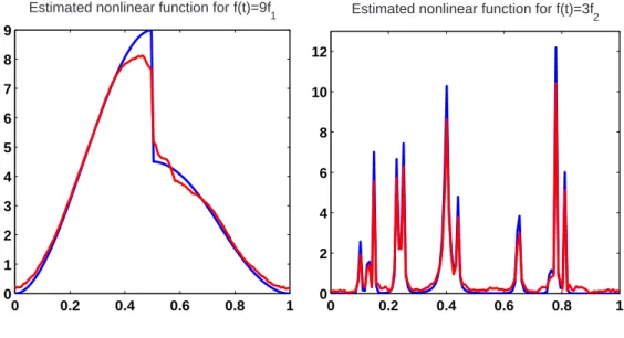
Alternatively, a grid could be used. In our simulation N = 128 or 256. Figure 2 depicts the estimated curves of f(t) for two different nonparametric cases based on the BIC and
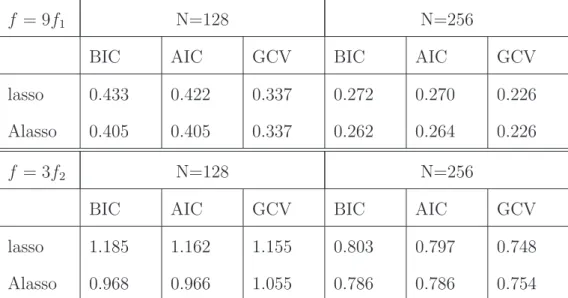
Table 3: Median of RASE values for the simulation study for the non-parametric component of the PLM, for functions f = 9f1 and f = 3f2.
f = 9f1 N=128 N=256
BIC AIC GCV BIC AIC GCV
lasso 0.433 0.422 0.337 0.272 0.270 0.226
Alasso 0.405 0.405 0.337 0.262 0.264 0.226
f = 3f2 N=128 N=256
BIC AIC GCV BIC AIC GCV
lasso 1.185 1.162 1.155 0.803 0.797 0.748
Alasso 0.968 0.966 1.055 0.786 0.786 0.754
for sample size 128. Table 3 summarizes the RASE for all different situations. It is shown that for the piecewise polynomial function f1, for the estimation of nonparametric compo-nent, the lasso method performs as well as the adaptive lasso in terms of RASE. For the more challenging bumps function f2, the adaptive lasso gives better RASE values over the simulation runs, with the difference becoming smaller for larger sample sizes.
5.3
Real example
We consider one of the case studies by Ruppert et al. (2003) aboutragweed pollen. The data were collected during the 1993 ragweed season in Kalamazoo, Michigan (USA). The develop-ment of accurate forecasting models for daily pollen levels is important for the treatdevelop-ment of pollen-related allergies. We consider the first 64 observations in the data set. The response
ragweed is the ragweed level for that day (grains/m3). There are four explanatory variables.
x1 = rain: indicator of significant rain for following day (1 = at least 3 hours of steady or brief but intense rain, 0 = otherwise),
0 0.2 0.4 0.6 0.8 1 0 1 2 3 4 5 6 7 8 9
Estimated nonlinear function for f(t)=9f
1 0 0.2 0.4 0.6 0.8 1 0 2 4 6 8 10 12
Estimated nonlinear function for f(t)=3f2
Figure 2: Estimated nonlinear function for f = 9f1 and f = 3f2.
x2 = temperature: temperature of the next day (oF),
x3 = wind: wind speed forecast for the next day,
x4 = day.in.seas: day number in the current ragweed pollen season.
The response ragweed is quite skewed, so we work with its square-root as Ruppert et al. (2003) suggested. The marginal relationships between the response and the other variables are shown in figure 3.
Since the day number in the current ragweed pollen season suggests a non-linear re-lationship with the level of ragweed pollen, we construct a partially linear model with a nonparametric component f(day.in.seas). It is also of interest to investigate whether the response variable has linear relationship with higher order effects of the variables wind and
0 1 0 5 10 15 rain sqrt of ragweed 40 50 60 70 80 90 0 5 10 15 20 temp sqrt of ragweed 0 5 10 15 0 5 10 15 20 wind sqrt of ragweed 0 20 40 60 80 0 5 10 15 20 day in season sqrt of ragweed
Figure 3: relationships between √ragweed and each possible predictor.
we fit for these data is
Y =β1x1+β2x2+β3x3+β4x22+β5x23+β6x1x3+f(day.in.seas) +ε.
We apply the proposed method to the data. The adaptive lasso with tuning parameters
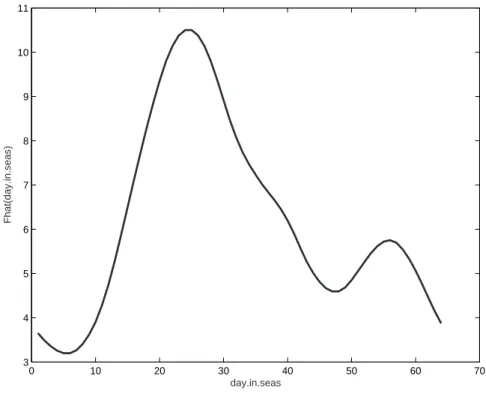
λ1 = 5.4996 andλ2 = 56.7 as determined by AIC, selected variables wind, and the square of temperature, with estimated coefficients 0.6454 and 2.3899, respectively. Both have positive coefficients, which indicates that the ragweed pollen level increases as the covariate increases. The other variables were not selected. The estimated nonparametric function ˆf(day.in.seas) is depicted in Figure 4.
0 10 20 30 40 50 60 70 3 4 5 6 7 8 9 10 11 day.in.seas Fhat(day.in.seas)
Figure 4: The estimated nonlinear function ˆf(day.in.seas) for the ragweed pollen data.
6
Discussion
In this paper, a flexible double penalized least squares estimator using sparse representations was proposed for partially linear modeling. The unified approach retains good features for simultaneous variable selection and model estimation. The sparse representation wavelet-based approach is able to estimate a broad class of functions, including functions that are nonsmooth.
We showed how to construct flexible regression models for a single continuous predictor modeled as a non-linear function, and all the other predictors entering the model linearly. However, in reality many regression problems involve several continuous covariates that may have non-linear relationships with the response. Our method can be readily extended through a backfitting approach to allow for additive nonparametric effects. That is, a model of the form
The iterative estimation method for the nonparametric part of the model would keep all but one component fixed to estimate the remaining functions, and then iterate until convergence. For future research one could derive the asymptotic distribution of the double penalized estimator, such that we can make inference about the linear coefficients as well as investigate the asymptotic behavior of the nonparametric part. It is expected that techniques combining the properties of thresholded wavelet fitting and the (adaptive) lasso estimator, will lead to such results. The rate of convergence of these estimators is another important issue that could be investigated.
References
Akaike, H. (1973). Maximum likelihood identification of Gaussian autoregressive moving average models. Biometricka, 60:255–265.
Chang, X. and Qu, L. (2004). Wavelet estimation of partially linear models. Computational statistics and data analysis, 47:31–48.
Cheng, F. (2005). On variance estimation in semiparametric regression models. Communi-cations in Statistics – Theory and Methods, 34:1737–1742.
Craven, P. and Wahba, G. (1979). Smoothing noisy data with spline functions. Numerische Mathematik, 31:377–403.
Donoho, D. L. and Johnstone, I. M. (1994). Ideal spatial adaptation via wavelet shrinkage.
Biometrika, 81:425–455.
Donoho, D. L. and Johnstone, I. M. (1995). Adapting to unknown smoothness via wavelet shrinkage. Journal of the American Statistical Association, 90:1200–1224.
Donoho, D. L., Johnstone, I. M., Kerkyacharian, G., and Picard, D. (1995). Wavelet shrink-age: Asymptopia. Journal of the Royal Statistical Society, Series B, 57:301–337.
Efron, B., Hastie, T., Johnstone, I., and Tibshirani, R. (2004). Least angle regression. The Annals of Statistics, 32:407–489.
Fadili, M. (2005). Penalized partially linear models using sparse representations with an application to fMRI time series. IEEE Transactions on Signal Processing, 53:3436–3448.
Fadili, M. and Bullmore, E. (2004). Penalized partially linear models using orthonormal wavelet bases with an application to fMRI time series. Biomedical Imaging: Nano to Macro, 2004. IEEE International Symposium on, 2:1171–1174.
Fan, J. and Li, R. (2001). Variable selection via nonconvave penalized likelihood and its oracle properties. Journal of the American Statistical Association, 96:1348–1360.
Fu, W. J. (1998). Penalized regression: the bridge versus the lasso. Journal of computational and graphical statistics, 7(3):397–416.
Hamilton, S. A. and Truong, Y. K. (1997). Local linear estimation in partly linear models.
Journal of Multivariate Analysis, 60:1–19.
H¨ardle, W., Liang, H., and Gao, J. (2000). Partially Linear Models. Springer Verlag. Heckman, N. (1986). Spline smoothing in partly linear models. Journal of the Royal
Statis-tical Society, Series B, 48:244–248.
Jansen, M., Malfait, M., and Bultheel, A. (1997). Generalized cross validation for wavelet thresholding. Signal Processing, 56(1):33–44.
Knight, K. and Fu, W. (2000). Asymptotics for lasso-type estimators. The Annals of Statistics, 28(5):1356–1378.
Li, R. and Liang, H. (2008). Variable selection in semiparametric regression modeling. The Annals of Statistics, 36(1):261–286.
Mallows, C. (1973). Some comments on Cp. Technometrics, 15:661–675.
Nason, G. P. (1996). Wavelet shrinkage using cross validation.Journal of the Royal Statistical Society, Series B, 58:463–479.
Rice, J. (1986). Concergence rates for partially splined models. Statistics and Probability Letters, 4:203–208.
Ruppert, D., Wand, M. P., and Carroll, R. J. (2003). Semiparametric Regression. Cambridge University Press.
Schwarz, G. (1978). Estimating the dimension of a model. The Annals of Statistics, 6:461– 464.
Simonoff, J. S. and Tsai, C.-L. (1999). Semiparametric and additive model selection using an improved Akaike information criterion.Journal of Computational and Graphical Statistics, 8(1):22–40.
Speckman, P. (1988). Kernel smoothing in partial linear models. Journal of the Royal Statistical Society, Series B, 50:413–436.
Tibshirani, R. and Saunders, M. (2005). Sparsity and smoothness via the fused lasso. Journal of the Royal Statistical Society, Series B, 67(1):91–108.
Tibshirani, R. J. (1996). Regression shrinkage and selection via the lasso. Journal of the Royal Statistical Society, Series B, 58:267–288.
Wang, H., Li, G., and Tsai, C. L. (2007). Regression coefficient and autoregressive or-der shrinkage and selection via lasso. Journal of the Royal Statistical Society, Series B, 69,part1:63–78.
Zhang, H. H. and Lu, W. (2007). Adaptive-lasso for Cox’s proportional hazards model.
Biometrika, 94:691–703.
Zhao, P. and Yu, B. (2006). On model selection consistency of Lasso. Journal of Machine Learning Research, 7:2541–2563.
Zou, H. (2006). The adaptive lasso and its oracle properties. Journal of the American Statistical Association, 101(476):1418–1429.
Zou, H., Hastie, T., and Tibshirani, R. (2007). On the “degrees of freedom” of the lasso.