Estimating long memory in volatility
Clifford M. Hurvich∗ Eric Moulines† Philippe Soulier†‡
Abstract
We consider semiparametric estimation of the memory parameter in a model which in-cludes as special cases both the long-memory stochastic volatility (LMSV) and fractionally integrated exponential GARCH (FIEGARCH) models. Under our general model the loga-rithms of the squared returns can be decomposed into the sum of a long-memory signal and a white noise. We consider periodogram-based estimators using a local Whittle criterion function. We allow the optional inclusion of an additional term to account for possible cor-relation between the signal and noise processes, as would occur in the FIEGARCH model. We also allow for potential nonstationarity in volatility, by allowing the signal process to have a memory parameterd∗≥1/2. We show that the local Whittle estimator is consistent
ford∗ ∈(0,1). We also show that the local Whittle estimator is asymptotically normal for d∗∈(0,3/4), and essentially recovers the optimal semiparametric rate of convergence for this
problem. In particular if the spectral density of the short memory component of the signal is sufficiently smooth, a convergence rate ofn2/5−δ ford∗∈(0,3/4) can be attained, where n is the sample size andδ > 0 is arbitrarily small. This represents a strong improvement over the performance of existing semiparametric estimators of persistence in volatility. We also prove that the standard Gaussian semiparametric estimator is asymptotically normal if
d∗= 0. This yields a test for long memory in volatility.
1
Introduction
There has been considerable recent interest in the semiparametric estimation of long memory in volatility. Perhaps the most widely used method for this purpose is the estimator (GPH) of Geweke and Porter-Hudak (1983). The GPH estimator of persistence in volatility is based on an ordinary linear regression of the log periodogram of a series that serves as a proxy for volatility, such as absolute returns, squared returns, or log squared returns of a financial time series. The single explanatory variable in the regression is log frequency, for Fourier frequencies in a neighborhood which degenerates towards zero frequency as the sample size n increases. Applications of GPH in the context of volatility have been presented in Andersen and Bollerslev (1997a,b), Ray and Tsay (2000), and Wright (2002), among others.
∗New York University : 44 W. 4’th Street, New York NY 10012, USA
†Ecole Nationale des T´el´ecommunications, 46 rue Barrault, 75005 Paris, France´ ‡Universit´e Paris X, 200 avenue de la R´epublique, 92001 Nanterre cedex, France
To derive theoretical results for semiparametric estimates of long memory in volatility, such as GPH, it is necessary to have a model for the series which incorporates some form of stochastic volatility. One particular such model is the long-memory stochastic volatility (LMSV) model of Harvey (1998) and Breidt, Crato and de Lima (1998). The LMSV model for a weakly stationary series of returns {rt}takes the form rt= exp(Yt/2)et where{et} is a series of i.i.d. shocks with
zero mean, and {Yt} is a weakly stationary linear long-memory process, independent of {et}, with memory parameter d∗ ∈(0,1/2). Under the LMSV model, the logarithms of the squared
returns,{Xt}={logr2t}, may be expressed as
Xt=µ+Yt+ηt, (1.1) where µ =E[loge2t] and {ηt} = {loge2t −E[loge2t]} is an i.i.d. process with variance ση2,
inde-pendent of{Yt}.
Another model for long memory in volatility is the fractionally integrated exponential GARCH (FIEGARCH) model of Bollerslev and Mikkelsen (1996). This model builds on the exponential GARCH (EGARCH) model of Nelson (1991). Bollerslev and Mikkelsen (1999) study FIE-GARCH forecasts of volatility, while Baillie, Cecen and Han (2000) study high frequency data using FIEGARCH. The weakly stationary FIEGARCH model takes the form rt =σtet, where
the{et} are i.i.d. with zero mean and a symmetric distribution, and logσt2=ω+
∞ X
j=1
ajg(et−j) (1.2)
withg(x) =θx+γ(|x| −E|et|),ω >0,θ∈R,γ ∈R, and real constantsaj such that the process logσt2 has long memory with memory parameterd∗ ∈(0,1/2). Ifθ is nonzero, the model allows for a so-called leverage effect, whereby the sign of the current return may have some bearing on the future volatility. As was the case for the LMSV model, here we can once again express the log squared returns as in (1.1) withµ=E[loge2t] +ω,ηt= loget2−E[loge2t], andYt= logσt2−ω.
Here, however, the processes {Yt}and {ηt}are not mutually independent.
In view of our goal of semiparametric estimation of d∗, we allow more generality in our
specification of the weights aj than Bollerslev and Mikkelsen (1996), who used weights
corre-sponding to a fractional ARIMA model. As far as we are aware, no theoretical justification of any semiparametric estimator ofd∗ has heretofore been presented for the FIEGARCH model.
Assuming that the volatility series{Yt}is Gaussian, Deo and Hurvich (2001) derived
asymp-totic theory for the GPH estimator based on log squared returns in the LMSV model. This provides some justification for the use of GPH for estimating long memory in volatility. Nev-ertheless, it can also be seen from Theorem 1 of Deo and Hurvich (2001) that the presence of the noise term {ηt} induces a negative bias in the GPH estimator, which in turn limits the
number m of Fourier frequencies which can be used in the estimator while still guaranteeing
√
m-consistency and asymptotic normality. This upper bound, m = o[n4d∗/(4d∗+1)], becomes increasingly stringent as d∗ approaches zero.
Another popular estimator of the memory parameter is the Gaussian semiparametric estima-tor (GSE), introduced by K¨unsch (1987), and later studied by Robinson (1995b) for processes
which are linear in a Martingale difference sequence. For the LMSV model, results analogous to those of Deo and Hurvich (2001) were obtained by Arteche (2003) for the GSE estimator, based once again on log squared returns. The use of GSE instead of GPH allows the assumption that {Yt} in (1.1) is Gaussian to be weakened to linearity in a Martingale difference sequence.
Arteche (2003) requires the same restriction on m as in Deo and Hurvich (2001).
Sun and Phillips (2003) proposed a nonlinear log-periodogram regression estimator ˆdNLP
of d∗, using Fourier frequencies 1, . . . , m. They partially account for the noise term {η
t} in
(1.1), through a first-order Taylor expansion about zero of the spectral density of the observa-tions. They establish the asymptotic normality ofm1/2( ˆd
NLP−d∗) under assumptions including
n−4d∗
m4d∗+1/2
→Const. Thus, ˆdNLP, with a variance of order n−4d∗/(4d∗+1/2)
, converges faster than the GPH estimator, but still arbitrarily slowly if d∗ is sufficiently close to zero. Sun and Phillips (2003) also assumed that the noise and signal are Gaussian. This rules out most LMSV models, since loge2
t is typically non-Gaussian.
Recently, Hurvich and Ray (2003) have proposed a local Whittle estimator ofd∗, based on log
squared returns in the LMSV model. The local Whittle estimator, defined precisely in Section 2.1, may be viewed as a generalized version of the GSE estimator. Hurvich and Ray (2003) included an additional term in the Whittle criterion function to account for the contribution of the noise term{ηt} in (1.1) to the low frequency behavior of the spectral density of{Xt}. The estimator is obtained from numerical optimization of the criterion function. It was found in the simulation study of Hurvich and Ray (2003) that the local Whittle estimator can strongly outperform GPH, especially in terms of bias whenm is large.
We assume that the observed process {Xt} is the sum of a long-memory signal {Yt} which
is linear in a Martingale difference sequence {Zt}, and a white noise {ηt} which is potentially contemporaneously correlated with{Zt}. Our signal plus noise model, made precise in Section
2 below, includes both the LMSV and FIEGARCH models as special cases, by allowing a contemporaneous correlation between the shocks in the signal and noise processes.
Many empirical studies have found estimates of the memory parameter in the log-squared returns, d∗, which are close to or even greater than 1/2, indicating possible nonstationarity of volatility. For example, Hurvich and Ray (2003) obtained a value of the local Whittle estimator
ˆ
dn= 0.556 for the log squared returns of a series of Deutsche Mark / US Dollar exchange rates
with n= 3485 andm =n0.8. In analyzing a similar data set with a parametric LMSV model, Harvey (1998), who explicitly allowed for the nonstationary case in his definition of the model, obtained an estimated memory parameter of 0.868. In view of these empirical findings, we allow in this paper for the possibility thatd∗exceeds 1/2. Specifically, we assume here thatd∗ ∈(0,1). In the context of our general signal plus noise model, allowing all of the generalizations described above, we will show that under suitable conditions our local Whittle estimator ˆdn
based on the firstmFourier frequencies is consistent. Then, we will establish the√m-consistency and asymptotic normality of ˆdn ford∗ ∈(0,3/4).
As long as the spectral density of the volatility (signal) process is sufficiently regular, our asymptotic results are free of upper restrictions on m arising from the presence of the noise
term. In particular, if the spectral density of the short memory component of the signal is twice differentiable, then we obtain asymptotic normality of √m( ˆdn −d∗) if m = [nζ] with
0 < ζ < 4/5. This represents a strong improvement over the GPH and GSE estimators of persistence in volatility and over the NLP regression estimator of Sun and Phillips (2003).
Since we use the Whittle likelihood function we are able to avoid the assumption that the signal is Gaussian. This assumption was required by Deo and Hurvich (2001), but many prac-titioners working with stochastic volatility models find the assumption to be overly restrictive.
The remainder of this paper is organized as follows. In Section 2.1, we define the local Whittle estimator ˆdn. Section 3 presents results demonstrating the consistency of the local Whittle estimator of bothd∗ and of the auxiliary parameterθ∗. Section 4 gives a central limit
theorem for ˆdn. The estimates of the parameters (d∗, θ∗) converge at different rates, and in the
case of the estimates ofθ∗the rates depend on d∗. Fortunately, however, the limiting covariance
matrix of a suitably normalized vector of parameter estimates does not depend onθ∗. We present
an expression, in terms of d∗, for the variance of the asymptotic distribution of √m( ˆd
n−d∗).
In Section 5, we prove that the standard GSE, without any of the additional terms considered in our local Whittle estimator, is asymptotically normal if d∗ = 0. This yields a test for long memory in volatility. In Section 6 we report the results of a simulation study on the properties of the local Whittle estimator.
2
Definitions and notations
We generalize the model (1.1) to a potentially nonstationary signal plus noise model, in which the observed process is either
Xt=
½
µ+Yt+ηt, (stationary case)
µ+Pts=1Ys+ηt, (nonstationary case), (2.1)
{Yt}is a weakly stationary zero mean process and{ηt}is a zero mean white noise with variance
σ2
η. Our main concern in this paper is the memory parameter of {Xt}, denoted by d∗. The
stationary case corresponds to d∗ ∈ (0,1/2) and the nonstationary case corresponds to d∗ ∈
[1/2,1).
In the stationary case, we lose no generality in assuming that {Yt} has zero mean, since
the estimators considered in this paper are all functions of the periodogram at nonzero Fourier frequencies. In the nonstationary case, the assumption that {Yt} has mean zero ensures that
{Xt} is free of linear trends. This does entail some loss of generality, but our estimator, which
makes no use of differencing or tapering, is not invariant to such trends, and would presumably be adversely affected by them. In any case, deterministic trends in volatility are perhaps somewhat artificial from an economic standpoint.
We now present precise assumptions on the signal process {Yt}. We assume first that the
respect to a zero mean, unit variance white noise (i.e. an uncorrelated second order stationary sequence){Zt}: Yt= X j∈Z ajZt−j, (2.2) withPj∈Za2
j <∞. In order to guarantee that the returns are a Martingale difference sequence,
one could assume thataj = 0 (j≤0). This assumption would imply that{rt}is adapted to the
natural filtration {Ft}of {et, Zt},Y is predictable with respect to this filtration and
E[rt| Ft−1] = exp(Yt/2)E[et] = 0.
We do not make such an assumption here, in order to consider the problem in its fullest gener-ality. Thus, we do not require the returns to be a Martingale difference sequence. Additional assumptions on {Zt} will be specified as needed.
We define a(x) =Pj∈Zajeijx and assume that it can be expressed as
a(x) = (1−eix)−dYa∗(x), x∈[−π, π]\ {0},
where dY ∈[−1/2,1/2), a∗ is a function that is continuous at 0, and a∗(0)6= 0. The quantity
dY is the memory parameter of the time series {Yt}. The stationary case corresponds to dY ∈
(0,1/2), and the nonstationary case corresponds to dY ∈ [−1/2,0). The case dY = 0, which
corresponds to short memory in volatility, will be addressed separately in Section 5. The spectral density of {Yt}is given by fY(x) =|a(x)|2/(2π), and can be expressed as
fY(x) =|1−eix|−2dYf∗
Y(x), (2.3)
withf∗
Y(x) =|a∗(x)|2/(2π).
The concept of pseudo spectral density has been defined for nonstationary processes. See, e.g., Solo (1992), Hurvich and Ray (1995), Velasco (1999). To generalize this concept so that it applies to our signal plus noise process {Yt}, we first state additional assumptions on the second-order dependence structure of the bivariate sequence {Zt, ηt}. Specifically, we assume
that:
∀t∈Z, E[ηtZt] =ρη ση and ∀s6=t, E[ηsZt] = 0. (2.4) The parameter ρη accounts for the possible contemporaneous correlation between Zt and ηt,
assumed constant. One such example is the FIEGARCH model with standard Normal multi-plying shocks, for whichηt= log(e2t)−E[log(et2)], Zt=θet+γ(|et| −
p
2/π), and {et} is i.i.d.
N(0,1), and (2.4) is in force. Since we assume E[Z2
t] = 1, θ and γ are linked by the relation
θ2+γ2(1−2/π) = 1. In that case,ρη =γcov(|e0|,log(e20))/ση, where ση2=π2/2.
In general, the spectral density or pseudo spectral density of the process {Xt} defined in (2.1) is then fX(x) = ( fY(x) + 2ρηση 2π Re(a(x)) + σ2 η 2π, (stationary case), |1−eix|−2f Y(x) + 2ρ2πησηRe((1−eix)−1a(x)) +σ 2 η 2π, (nonstationary case). (2.5)
In both cases, under additional smoothness assumption on the behavior ofa∗ about 0 (that will
be made precise in the next section),fX admits the following expansion at 0:
fX(x)∼x−2d ∗ fY∗(0) + Re ³ (1−eix)−d∗ ´2ρ ηση p f∗ Y(0) √ 2π + σ2 η 2π, (2.6) with d∗ = ½ dY ∈(0,1/2), (stationary case), dY + 1∈[1/2,1), (nonstationary case), (2.7) where the symbol ∼indicates that the ratio of the left hand side to the right hand side of the above formula tends to 1 as x→0+. Thus, in the stationary case, {X
t} has the same memory
parameter as {Yt}, namely dY, while in the nonstationary case {Xt} has the same memory
parameter as the partial sum of {Yt}, namely dY + 1.
Remark 2.1. In the stationary case where the returns are rt = eYt/2et, and Yt=
P∞
j=1ajZt−j,
Surgailis and Viano (2002) have proved that under the additional assumptions thatE[eu|Z1|]<∞
for all u > 0 and that {Zt} and {et} are i.i.d. sequences, the memory parameter of the series
{|rt|u}is the same as the memory parameter of{Yt}. Thus, for both the LMSV and FIEGARCH
models, under the above mentioned restrictions, the squared returns and the log-squared returns have the same memory parameter. In the nonstationary case, the relationship between these two memory parameters remains an open question.
2.1 The Local Whittle Estimator
Consider a covariance stationary process{Xt} with spectral density
fX(x) =|1−eix|−2d
∗ fX∗(x),
where d∗ ∈ (−1/2,1/2) and fX∗ is a positive function which is smooth in a neighborhood of the origin. The GSE estimator of d∗ consists in locally fitting a parametric model for f∗
X
by minimizing the Whittle contrast function. The parametric model used in GSE replaces
f∗
X by a constant. This method yields a consistent and asymptotically normal estimator of
d∗ ∈ (−1/2,1/2), under mild assumptions both on f∗
X and the process {Xt}. These results
were later extended to the nonstationary case d∗ ∈ [1/2,1) by Velasco (1999) who proved the
consistency ford∗ in this range and asymptotic normality ford∗ ∈[1/2,3/4).
In some situations however, the local-to-zero parameterization off∗
X(x) by a constant may be
inefficient. An example is the situation of a long-memory process observed in an additive noise. In order to improve the efficiency, one can try to fit a more complex local parametric model forf∗
X. In the local Whittle estimator, defined below in a general setting, fX∗(x) is replaced by
G(1 +h(d, θ, x)), where Gis a positive constant and h is a function tailored to the problem at hand. The additional parameter θ can be seen as a nuisance parameter which is included to allow some flexibility in the modelling off∗
The discrete Fourier transform and the periodogram ordinates of any process{Vt}evaluated
at the Fourier frequencies xj = 2jπ/n,j= 1, . . . , n, are respectively denoted by
dV,j= (2πn)−1/2 n
X
t=1
Vte−itxj, and IV,j=|dV,j|2.
The local Whittle contrast function, based on the observations X1, . . . , Xn, is defined as ˆ Wm(d, G, θ) = m X k=1 ( log ³ Gx−k2d(1 +h(d, θ, xk) ´ + IX,k Gx−k2d(1 +h(d, θ, xk)) ) (2.8) where m < n/2 is a bandwidth parameter (the dependence onn is implicit). ConcentratingG
out of ˆWm yields the following profile likelihood ˆ Jm(d, θ) = log à 1 m m X k=1 x2d k IX,k 1 +h(d, θ, xk) ! +m−1 m X k=1 log{x−k2d(1 +h(d, θ, xk))} = log à 1 m m X k=1 k2dI X,k 1 +h(d, θ, xk) ! +m−1 m X k=1 log{k−2d(1 +h(d, θ, xk))}. (2.9)
The local Whittle estimator is any minimand of the empirical contrast function ˆJm over the
admissible set Dn×Θn (which may depend on the sample sizen):
( ˆdn,θˆn) = arg min (d,θ)∈Dn×Θn
ˆ
Jm(d, θ). (2.10)
Note that ( ˆdn,θˆn) depends on h,Dn and Θn.
We now specify three different parameterizations that we will use for estimation of the memory parameter in the model (2.1).
(P0)
h(d, x)≡0, Dn= [−1/2,1]. (2.11) Here, there is no parameterθ and the definition of Θnis thus irrelevant. This parameter-ization is used for the GSE estimator.
(P1)
h(d, θ, x) =θx2d, Dn= [²n,1], Θn= [0, ²−n2], (2.12)
where {²n} is a sequence that tends to zero as n tends to infinity at a rate that will
be specified in the sequel. This parameterization is used for the local Whittle estimator in the LMSV model when ρη is known to be zero, as in Hurvich and Ray (2003). Our parameterization conforms with this model: indeed, the expansion (2.6) of the spectral (or
pseudo spectral) densityfX at 0 whenρη = 0 can be expressed asfX(x)∼x−2d ∗ f∗ Y(0)(1 + h(d∗, θ∗, x), withh as in (2.12) and θ∗= σ 2 η 2πf∗ Y(0) . (2.13)
Note that if d∗ ∈ (0,1), the definition of D
n and Θn implies that for all sufficiently large
n, we will have d∗ ∈ D n and θ∗ ∈Θn. (P2) h(d, θ, x) =θ1x2dRe ¡ (1−eix)−d¢+θ 2x2d, Dn= [²n,1], Θn= [−2²n−1,2²−n1]×[0, ²−n2], (2.14) where {²n} is as described above. This parameterization is used for the local Whittle
estimator whenρη is not required to be zero, as in the FIEGARCH model and the LMSV
model with contemporaneous correlation between{Zt}and{ηt}. Here again, the expansion (2.6) can be expressed as fX(x)∼x−2d ∗ fY∗(0)(1 +h(d∗, θ∗, x)), withh as in (2.14) and θ∗ = (θ1∗, θ∗2) with θ∗1 = p2ρηση 2πf∗ Y(0) and θ∗2 = σ 2 η 2πf∗ Y(0) . (2.15) We denote the local Whittle estimators associated with the parameterizations (P0), (P1) and (P2) by ( ˆd(i)n ,θˆ(i)n ),i= 0,1,2, respectively. Note that ˆd(0)n is simply the GSE estimator, based on
a parameterization which does not involve the noise term. In some of our discussions, as should be clear from the context, we reserve the term ”local Whittle estimator” to refer only to the parameterizations (P1) and (P2) but not (P0).
Remark 2.2. The presence of an ²n sequence tending to zero in parametrizations (P1) and (P2)
allows the admissible parameter space to depend on n and to become larger as n increases. This in turn will allow us to state and prove our main theoretical results without making arbitrary restrictions on the true parameters, as is done in much of the current literature (see, e.g., Robinson 1995b). Nevertheless, if we took ²n to be fixed and positive, then our main results would continue to hold as long as the true parameters lie in the corresponding admissible parameter space.
Remark 2.3. We explain here the (perhaps) surprising form of the parameterization (P2). For
x∈(0, π] andd∈(0,1), it is well known that|1−eix|−2d=x−2d(1 +O(x2)), but it should be noted that
Re
n
(1−eix)−d
o
={2 sin(x/2)}−dcos{d(x/2 +π/2)}=x−dcos(πd/2){1 +O(x)},
where the term O(x) cannot be improved. Replacing Re©(1−eix)−dªwith x−d in (P1) would
not only change the value of the parameterθ1, but also create a bias term that would result in a slower rate of convergence for ˆd(2)n (moreover depending on d∗) than the rate we will be able
Remark 2.4. The correction term h(d, θ, x) in parameterizations (P1) and (P2) is the key el-ement which allows us to attain a better rate of convergence for the local Whittle estimator, in comparison to the ordinary GSE and GPH estimators. Indeed, the use of h(d, θ) frees the optimal rate of convergence of the local Whittle estimator from an undesirable dependence on
d∗, a problem faced by the ordinary GPH estimator considered in Deo and Hurvich (2001).
3
Consistency of the local Whittle estimator
In order to prove consistency of the local Whittle estimator ˆdn, we consider the following
as-sumptions.
(H1){Zt}is a zero mean unit variance white noise such that 1 n n X t=1 (Zt2−1)−→P 0 (3.1) and for any (s, t, u, v)∈N4 such that s < tand u < v,E[|Z
uZvZsZt|]<∞ and
E[ZuZvZsZt] =
½
1 ifu=sand t=v
0 otherwise. (3.2)
Remark 3.1. This assumption is the weakest one under which we were able to construct our proof of consistency, and is satisfied under a variety of conditions. For instance, it is implied by assumption A3 of Robinson (1995b) which states that {Zt} is a martingale difference sequence
satisfying E[Z2
t|σ(Zs, s < t)] = 1 a.s. (which implies (3.2)) and strongly uniformly integrable
(which implies (3.1)). Note that (3.1) holds when{Zt2} is ergodic. Finally, note that (3.2) rules out the case s= t since it assumes that s < t and u < v, and therefore (3.2) does not imply thatE[Z4
t] = 1 (which would be impossible except for a Rademacher random variable).
For reference, we recall the assumption on{ηt}.
(H2){ηt} is a zero mean white noise with variance ση2 such that for each s6=t, E[ηsZt] = 0
and for each t,E[ηtZt] =ρηση.
Note thatρη is the correlation between Zt andηt, which is assumed to be constant. (H3) {Yt} admits the linear representation (2.2) and the function a(x) =
P
j∈Zajeijx can
be expressed for x ∈ [−π, π]\ {0} as a(x) = (1−eix)−dYa∗(x), where d
Y ∈(−1/2,1/2), a∗ is
integrable over [−π, π], a∗(−x) = a∗(x) for all x ∈[−π, π] and there exist ϑ∈(0, π], β ∈(0,2]
and µ >0 such that a∗ is differentiable at 0 ifβ >1 and for allx∈[−ϑ, ϑ],
|a∗(x)−a∗(0)| ≤µ|a∗(0)||x|β, β ∈(0,1] (3.3)
Remark 3.2. The function (1−eix)−d is defined ford∈(−1/2,1/2)\ {0}and x∈[−π, π]\ {0} by (1−eix)−d= ∞ X j=0 Γ(d+j) Γ(d)j! e ijx.
This series is absolutely convergent if d < 0 and converges in the mean square if d > 0. For
d= 0, we set (1−eix)0≡1. Since by assumptiona∗(−x) =a∗(x), thus|a∗|2 is an even function.
If moreover a∗ is differentiable at 0, thena∗0(0) = −a∗0(0) and for all β ∈(0,2], there exists a
constantC such that for allx∈[−ϑ, ϑ], it holds that
¯
¯|a∗(x)|2− |a∗(0)|2¯¯≤C|x|β. (3.5)
Remark 3.3. In the related literature (Robinson (1995b), Velasco (1999), Andrews and Sun (2001)), it is usually assumed moreover that the functionais differentiable in a neighborhood of zero, except at zero, with|xa0(x)|/|a(x)|bounded on this neighborhood. Hence our assumptions
are weaker than those of the above references.
Theorem 3.1. Assume (H1), (H2) and (H3) and d∗ ∈ [0,1). Let m be a non-decreasing sequence such that
lim
n→∞ ¡
m−1+m/n¢= 0, (3.6)
and set ²n= (log(n/m))−1/2. Then, the local Whittle estimators dˆ(i)n , i= 0,1,2 are consistent.
Remark 3.4. Arteche (2003), Theorem 1, proved the consistency ˆd(0)n (the GSE) for a
long-memory process observed in independent noise (with no contemporaneous correlation) in the stationary casei.e. ford∗∈(0,1/2). Theorem 3.1 extends this result to the nonstationary case d∗ ∈ (1/2,1) and to the case where the noise {η
t} is (possibly) contemporaneously correlated
with{Yt}, thus covering the FIEGARCH model. Furthermore, Theorem 3.1 implies that ˆd(1)n is
consistent even ifρη is nonzero.
Remark 3.5. The local Whittle estimator ˆd(i)n ,i= 1,2 is consistent ifd∗ = 0, but by construction
its rate of convergence is at most²n. The necessity of introducing the sequence ²n comes from
certain technicalities in the proof of Theorem 1. We do not know if it is possible to define
Dn= [0,1] under (P1) and (P2). In any case, ifd∗ = 0, the parameterθ∗need not be identifiable.
Thus, if a small value of ˆd(i)n is obtained, it should be better to test for d∗ = 0 by using the
standard GSE. We will establish the validity of this procedure in section 5.
Theorem 3.1 provides no information about the behavior of ˆθ(i)n , i= 1,2. This is because,
as n→ ∞, the objective function becomes flat as a function of θ. Thus a special technique is needed to prove the consistency of ˆθ(i)n , i= 1,2 which requires strengthened assumptions. This
technique was first used in a similar context by Sun and Phillips (2003). We now introduce these assumptions.
(H4) {Zt} is a martingale difference sequence such that for all t, E[Zt4] = µ4 < ∞ and
E[Z2
Remark 3.6. (H4)implies(H1). More precisely, it implies that{Z2
t −1} is a square integrable
martingale difference sequence and thatn−1Pn
t=1(Zt2−1) =OP(n−1/2).
(H5) {ηt} is a zero mean white noise with variance ση2 such that supt∈NE[ηt4]<∞, a.s. and
for all (s, t, u, v)∈N4 such that s < tand u < v,
E[ηuηvηsηt] = ½ σ4 η ifu=s andt=v 0 otherwise. (3.7) cum(Zt1, Zt2, ηt3, ηt4) = ½ κ ift1 =t2 =t3 =t4, 0 otherwise (3.8)
Theorem 3.2. Assume(H2),(H3),(H4)and(H5)andd∗ ∈(0,1). Letmbe a non-decreasing sequence of integers such that
lim n→∞ ³ m−4d∗−1+δn4d∗+n−2βm2β+1log2(m) ´ = 0 (3.9)
for some arbitrarily small δ >0 and set ²n = (log(n/m))−1/2. Then dˆ(i)
n −d∗ =OP((m/n)2d
∗
)
and θˆn(i)−θ∗ =oP(1), i= 1,2.
Remark 3.7. The first term in (3.9) imposes a lower bound on the allowable value ofm, requiring that m tend to ∞ faster than n4d∗/(4d∗+1)
. This condition can be fulfilled only whenβ > 2d∗.
Note thatβ >2d∗ always holds if β = 2, which is the most commonly accepted value for β. It is interesting that Deo and Hurvich (2001), assumingβ = 2, found that form1/2( ˆd
GP H−d∗) to
be asymptotically normal with mean zero, where ˆdGP H is the GPH estimator, the bandwidthm
must tend to∞ at a rateslower thann4d∗/(4d∗+1). Whenβ ≤2d∗, then it is no longer possible to prove that ˆθn is a consistent estimator of θ∗, and the proposed local Whittle estimator will
not perform better than the standard GSE.
4
Asymptotic normality of the local Whittle estimator
We focus here on ˆd(i)n and ˆθ(i)n , i= 1,2. Corresponding results for the GSE estimator will be
presented in Section 5. The main result of this section is Theorem 4.3, which is a central limit theorem for the vector of estimated parameters. Before presenting this main result, we outline the main steps in the proof, which are not completely standard due to the asymptotic flatness of the objective function.
For ease of notation here, in the discussion below, we omit the superscript in ˆd(i)n . Contrary
to standard statistical theory of minimum contrast estimators, the rates of convergence of ˆdn−d∗
and of ˆθn−θ∗ are different, whered∗ is defined in (2.7) andθ∗ is defined in (2.13) in the LMSV
case and (2.15) in the FIEGARCH case. To account for the difference in these rates, we prove thatD∗
n( ˆdn−d∗,θˆn−θ∗) is asymptotically normal with zero mean, whereDn∗ is a deterministic
diagonal matrix whose diagonal entries tend to ∞ at different rates, as defined below. Our proof starts with a second order Taylor expansion of the contrast function. The gradient of the
contrast function evaluated at the estimates vanishes, since they are consistent and converge to an interior point of the parameter set.
Denote Hn(d, θ) =
R1
0 ∇2Jˆm(d∗ +s(d−d∗), θ∗+s(θ−θ∗))ds. With this notation, a first
order Taylor expansion yields 0 =mD∗n−1∇Jˆm( ˆdn,θˆn) = mD∗n−1∇Jˆm(d∗, θ∗) +mD∗n−1Hn( ˆdn,θˆn)D∗n−1D∗n ³ ( ˆdn,θˆn)−(d∗, θ∗) ´ . (4.1) The next step is to prove thatmD∗
n−1∇Jˆm(d∗, θ∗) converges in distribution to a non-degenerate
Gaussian random variable with zero mean andmDn∗−1Hn( ˆdn,θˆn)Dn∗−1 converges in probability
to a non-singular matrix. This is stated in the following two propositions.
Proposition 4.1. Assume (H2), (H3), (H4) and(H5). Ifd∗ ∈(0,3/4),β >2d∗ and m is a non-decreasing sequence of integers such that (3.9)holds, thenmD∗
n−1∇Jˆm(d∗, θ∗) converges to
the Gaussian distribution with zero mean and variance Γ∗ with (i) D∗n=m1/2Diag¡1, x2dm∗¢and
Γ∗= Ã 4 − 4d∗ (1+2d∗)2 − 4d∗ (1+2d∗)2 4d ∗2 (1+2d∗)2(1+4d∗) !
under (P1), assuming ρη is known to be 0;
(ii) D∗ n=m1/2Diag ¡ 1, xd∗ m/cos(πd∗/2), x2d ∗ m ¢ and Γ∗ = 4 − 2d∗ (1+d∗)2 − 4d ∗ (1+2d∗)2 − 2d∗ (1+d∗)2 2d ∗2 (1+d∗)2(1+2d∗) 2d ∗2 (1+d∗)(1+2d∗)(1+3d∗) − 4d∗ (1+2d∗)2 2d ∗2 (1+d∗)(1+2d∗)(1+3d∗) 4d ∗2 (1+2d∗)2(1+4d∗) under (P2).
Proposition 4.2. Assume (H2), (H3) and (H4). If d∗ ∈ (0,3/4), β > 2d∗ and m is a non-decreasing sequence of integers that satisfies (3.9), then mD∗
n−1Hn(d, θ)Dn∗−1 converges in
probability toΓ∗, uniformly with respect to(d, θ)∈ {d: |d−d∗| ≤log−5(m)} ×Θ, with D∗
n and
Γ∗ defined as in Proposition 4.1.
Remark 4.1. An important feature is that Γ∗ does not depend on the parameter θ∗. This was
already noticed by Andrews and Sun (2001) in the context of local polynomial approximation. Since the matrix Γ∗ is invertible, the matrixD∗
n−1Hn( ˆdn,θˆn)Dn∗−1 is invertible, with probability
tending to one. Hence (4.1) yields:
D∗n ³ ( ˆdn,θˆn)−(d∗, θ∗) ´ =− n mD∗n−1Hn( ˆdn,θˆn)D∗n−1 o−1 mD∗n−1∇Jˆm(d∗, θ∗).
This and Propositions 4.1 and 4.2 yield our main result. Recall that our estimators are defined in section 2.1 with²n= (log(n/m))−1/2.
Theorem 4.3. Assume (H2), (H3), (H4), (H5), d∗ ∈(0,3/4), β >2d∗ and let m be a non-decreasing sequence of integers that satisfies (3.9). Then, under (P1), assuming ρη is known to
be zero, D∗
n
³
( ˆd(1)n ,θˆn(1))−(d∗, θ∗)
´
is asymptotically Gaussian with zero mean and covariance matrix Γ∗−1 = (1 + 2d∗)2 16d∗2 Ã 1 1+4dd∗∗ 1+4d∗ d∗ (1+2d ∗)2(1+4d∗) d∗2 ! . Under (P2), D∗ n ³ ( ˆd(2)n ,θˆn(2))−(d∗, θ∗) ´
is asymptotically Gaussian with zero mean and covari-ance matrix Γ−1= 1 16d∗4 0 B @ −1 0 0 0 2(1+d∗) d∗ 0 0 0 1+22d∗d∗ 1 C A × 0 @ (1 +d ∗)2(1 + 2d∗)2 −2(1 +d∗)(1 + 2d∗)2(1 + 3d∗) (1 +d∗)(1 + 2d∗)(1 + 3d∗)(1 + 4d∗) −2(1 +d∗)(1 + 2d∗)2(1 + 3d∗) 4(1 +d∗)2(1 + 2d∗)(1 + 3d∗)2 −2(1 +d∗)(1 + 2d∗)2(1 + 3d∗)(1 + 4d∗) (1 +d∗)(1 + 2d∗)(1 + 3d∗)(1 + 4d∗) −2(1 +d∗)(1 + 2d∗)2(1 + 3d∗)(1 + 4d∗) (1 + 2d∗)2(1 + 3d∗)2(1 + 4d∗) 1 A × 0 B @ −1 0 0 0 2(1+d∗d∗) 0 0 0 1+22d∗d∗ 1 C A.
Corollary 4.4. Under the assumptions of Theorem 4.3, m1/2( ˆd(1)
n −d∗) is asymptotically
Gaus-sian with zero mean and variance
(1 +d∗)2 16d∗2
if ρη is known to be 0; and m1/2( ˆd(2)n −d∗) is asymptotically Gaussian with zero mean and
variance
(1 +d∗)2(1 + 2d∗)2
16d∗4 .
Remark 4.2. It is seen that the local Whittle estimator ˆd(i)n ,i= 1,2 is able to attain the same
rate of convergence under the signal plus noise model (1.1) as that attained by the standard GSE d(0)n in the case of no noise, as long as β >2d∗.
Remark 4.3. The asymptotic variance of ˆd(i)n increases when d∗ is small, but this loss is
com-pensated by the gain in the rate of convergence with respect to the standard GSE (and GPH).
5
Asymptotic normality of the standard GSE
Theorem 3.1 states that the GSE is consistent if d∗ ∈ (0,1). We now state that it is
asymp-totically normal if d∗ ∈ (0,3/4) but with a rate of convergence slower than the local Whittle estimator considered above.
Theorem 5.1. Under the assumptions of Theorem 4.3, ifd∗ ∈(0,3/4) andm satisfies
lim n→∞ ³ m−1+m2γ∗+1n−2γ∗ ´ = 0, (5.1)
with γ∗ =d∗ if ρ
η 6= 0 and γ∗ = 2d∗ if ρη = 0; then m1/2( ˆd(0)n −d∗) is asymptotically normal
with variance 1/4.
Remark 5.1. If ρη is zero, then (5.1) requires that m=o(n4d
∗/(4d∗+1)
), so the upper bound on
m to ensure √m-consistency of GSE is essentially the same as that required for GPH by Deo and Hurvich (2001). If, however, ρη 6= 0, then the upper bound onm for GSE becomes more
stringent,m=o(n2d∗/(2d∗+1)
), since the nonzero value ofρη increases the asymptotic bias of the
GSE. Similar restrictions would presumably apply in this situation for GPH.
Whend∗ = 0, the theory of Robinson (1995b) cannot be directly applied to prove consistency
and asymptotic normality of ˆd(0)n , since the process Xt =Yt+ηt is not necessarily linear with
respect to a martingale difference sequence. Nevertheless, if we strengthen the assumptions on the noise{ηt}, we can prove the consistency and asymptotic normality of ˆd(0)n whendY =d∗= 0.
Theorem 5.2. Assume thatd∗=d
Y = 0,(H2),(H3),(H4), (H5)and thatη is a martingale
difference sequence that satisfies
cum(Zu, Zv, Zs, ηt) =γ if s=t=u=v and 0 otherwise. (5.2)
Ifmis a non-decreasing sequence of integers that satisfieslimn→∞(m−1+n−2βm2β+1log2(m)) =
0, then m1/2dˆ(0)
n is asymptotically Gaussian with zero mean and variance 1/4.
These results yield a test for long memory in volatility based on the standard GSE estimator, since Theorem 5.2 gives the asymptotic distribution ofm1/2dˆ(0)
n under the null hypothesisd∗ = 0
and Theorem 5.1 shows thatm1/2dˆ(0)
n → ∞ifd∗>0. Another test for long memory in volatility,
based on the ordinary GPH estimator, was justified by Hurvich and Soulier (2002). Since the ratio of the asymptotic variances of the GPH and GSE estimators isπ2/6, the test based on the
GSE estimator should have higher local power than the one based on GPH.
6
Simulations
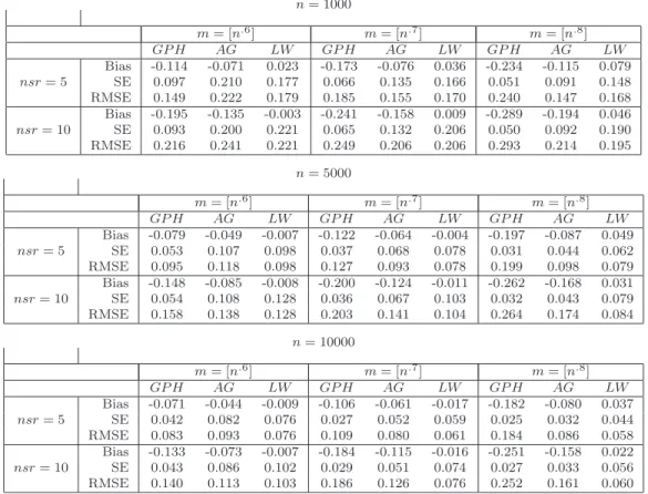
We present here some simulation results on the performance of the proposed local Whittle estimator, denoted here by LW. A comprehensive simulation study on the LW estimator was performed by Hurvich and Ray (2003), who included a proposal for constructing accurate finite-sample standard errors forLW. The concise set of results we present here was generated in the preparation of Hurvich and Ray (2003), but not reported there due to lack of space.
For each of three sample sizes (n= 1000,n= 5000, n= 10000), and for each of two values (nsr = 5, nsr = 10) of the noise to signal ratio nsr = σ2
η/(2πfY∗(0)), 1000 realizations were
generated from an LMSV model with standard Gaussian shockse, and signal process{Yt}given
by the ARFIMA(1, d∗,0) model (1−B)d∗
(1−φB)Yt =Zt, where φ= 0.8 and d∗ = 0.4. The
innovations Zt were iid Gaussian with mean zero, and variance chosen such that the specified
likelihood (2.9) with parameterization (2.12) was minimized, ford∈[.01, .75] and θ∈[e−8, e20].
Note that the admissible parameter space here does not depend onn, so the²nsequence is fixed.
See Remark 2.2.
Table 1 reports the bias, standard error (SE) and root mean squared error (RMSE) for LW, as well as the GPH estimator of Geweke and Porter Hudak (1983), and the bias reduced local polynomial log periodogram regression estimator of Andrews and Guggenberger (2003), denoted by AG. It was shown in Andrews and Guggenberger (2003) that the AG estimator has improved bias properties compared to GPH for Gaussian processes if the spectral density of the observations is sufficiently smooth. We used the simplest version of AG, in which a single additional term x2
j is included in the log periodogram regression. All three estimates of the
memory parameter were constructed from the simulated log squared return series, {Xt}t. For
each realization and each estimator, three different bandwidths were considered (m = [n0.6],
m= [n0.7],m= [n0.8]).
Both GPH and AG suffer from negative bias, which worsens significantly as m or nsr is increased, presumably due to the noise term η that neither of these estimators was designed to explicitly account for. On the other hand, the bias of LW is stable with respect to nsr, and increases only modestly inm, due to the autoregressive component in the model. In most cases, LW is the best estimator in terms of RMSE, though LW has a higher standard error than GPH and AG. Overall, these results are consistent with existing theory.
APPENDIX: Proofs
The estimators introduced in section 2.1 are minimum contrast estimators. Empirical pro-cesses are the main tools in the study of such estimators. Since the Whittle contrast is based on the spectral density of a second order stationary time series, the empirical process involved is often referred to as the empirical spectral process. See for instance Dahlhaus and Polonik (2002) or Soulier (2002). In the first section of this appendix, we state two Propositions which provide the tools to derive the asymptotic properties of minimum contrast estimators: a uniform weak law of large numbers and a central limit theorem for the spectral empirical process. Their proof is very technical and is postponed to Appendix F. Using these tools, we prove our main results in the following sections. Appendix B and C deal with the main statistical issues of this paper, namely the consistency of the estimators ofd∗andθ∗. The proof of the consistency of ˆd
n, in
Ap-pendix B, is essentially the same as the original proof of Robinson (1995b), but is more concise here thanks to the use of Proposition A.1. The proof of the consistency of ˆθn, in Appendix C
is rather involved. We have tried to make it clear, though concise. It is the longest and more difficult part of this proof. Appendices D and E contain the proof of the asymptotic normality results, which are quite standard and made very short by again referring to Propositions A.1 and A.2.
A
Results for the empirical spectral process
Define
fX,k =x−2d
∗
k fY∗(0){1 +h(d∗, θ∗, xk)} (A.1)
where the function h is defined either in (P0), (P1) or (P2), and for a positive integerm and
c= (c1, . . . , cm)∈Rm, Zm(c) = m X k=1 ck{fX,k−1IX,k−1}. (A.2)
For²∈(0,1] andK >0, let Cm(², K) be the subset of vectors c∈Rm such that
for all k∈ {1, . . . , m−1}, |ck−ck+1| ≤Km−²k²−2, |cm| ≤Km−1. (A.3)
Proposition A.1 (Uniform weak law of large numbers).
1. Assume (H1), (H2)and (H3). Letm be a non-decreasing sequence of integers such that
limn→∞{m n−1 +m−1} = 0. Then, for any ² ∈ (0,1), any constant K < ∞ and any d∗ ∈(0,1),
sup
c∈Cm(²,K)
2. Assume moreover that (H4), (H5)and one of the following assumptions hold.
(2.i) h is given by (P1), ρη = 0, d∗ ∈(0,3/4)and m satisfies
lim n→∞ ³ m−1+m2β+1log2(n)n−2β ´ = 0; (A.4)
(2.ii) h is given by (P2), d∗ ∈(0,3/4)and m satisfies (A.4); (2.iii) h≡0, d∗ ∈(0,3/4)and m satisfies
lim n→∞ ³ m−1+m2γ∗+1n−2γ∗ ´ = 0, (A.5) with γ∗ =d∗ if ρ η 6= 0 and γ∗= 2d∗ if ρη = 0; (2.iv) d∗ = 0, h ≡ 2ρ ηση/ p f∗
Y(0)/(2π) +ση2/(2πfY(0)), η satisfies the assumptions of
Theorem 5.2 and m satisfies (A.4).
Then for all ²∈(0,1]there exists a constant C such that, for all K >0
E " sup c∈Cm(²,K) |Zm(c)| # ≤CKm−(1/2∧²)logδ(m), (A.6)
withδ = 1 if ²= 1/2 and δ= 0 otherwise.
Proposition A.2. Assume (H2),(H3), (H4)and(H5). Letm be a non-decreasing sequence of integers and let (cm,k)1≤k≤m be a triangular array of real numbers that satisfy
m X k=1 cm,k = 0 and m X k=1 c2m,k = 1 (A.7) lim n→∞ nXm k=1 |cm,k−cm,k+1|+|cm,n| o2 log(n) = 0. (A.8)
Assume either (2.i), (2.ii), (2.iii) or (2.iv) of Proposition A.1. Then Pmk=1cm,kfX,k−1IX,k is
asymptotically standard Gaussian.
B
Proof of Theorem 3.1 and of the consistency part of
Theo-rem 5.2
In this section, we prove Theorem 3.1 and the consistency part of Theorem 5.2. This proof only uses the first part of Proposition A.1, and is valid for each of the four cases considered. The only difference between them is the remainder termRm(d, θ) (defined below) which is identically
the case of the local Whittle estimator. Therefore, we omit the superscript in the notation of the estimators. Define
D1,n= (−∞, d∗−1/2 +²)∩ Dn, (B.1)
D2,n= [d∗−1/2 +²,+∞)∩ Dn (B.2)
where² <1/4 is a positive real number to be set later andDnis defined in (2.11), (2.12) or (2.14). As originally done in Robinson (1995b), we separately prove that limn→∞P( ˆdn∈ D1,n) = 0 and
that ( ˆdn−d∗)1D2,n( ˆdn) tends to zero in probability. Note that D1,n is empty if it is assumed
thatd∗∈(0,1/2) and²is chosen small enough. We first prove that ( ˆd
n−d∗)1D2,n( ˆdn) tends to
zero in probability. Denote
αk(d, θ) = 1 +h(d ∗, θ∗, x k) 1 +h(d, θ, xk) , γm,k(d, θ) = k2d−2d ∗ αk(d, θ) Pm j=1j2d−2d ∗ αj(d, θ) , γm(d, θ) = (γm,k(d, θ))1≤k≤m, Jm(d, θ) = log à 1 m m X k=1 x2dk −2d∗αk(d, θ) ! + 1 m m X k=1 log ³ x−k2d{1 +h(d, θ, xk)} ´ .
With this notation and the notation introduced in Appendix A, we get: ˆ
Jm(d, θ) = log(1 +Zm(γm(d, θ))) +Jm(d, θ) + log(fY∗(0)). (B.3)
Due to the strict concavity of the log function, for any positive integer m and positive real numbersa1, . . . , am, it holds that
log à 1 m m X k=1 ak ! ≥ 1 m m X k=1 log(ak). Thus, (d∗, θ∗) minimizesJ
m. Moreover, by definition, ( ˆdn,θˆn) minimizes ˆJm. Hence on the event
{dˆn∈ D2,n}, 0≤Jm( ˆdn,θˆn)−Jm(d∗, θ∗) =Jm( ˆdn,θˆn)−Jˆm( ˆdn,θˆn) + ˆJm( ˆdn,θˆn)−Jˆm(d∗, θ∗) + ˆJm(d∗, θ∗)−Jm(d∗, θ∗) ≤log{1 +Zm(γm(d∗, θ∗))} −log{1 +Zm(γm( ˆdn,θˆn))} (B.4) ≤2 sup (d,θ)∈D2,n×Θn |log{1 +Zm(γm(d, θ))}|. (B.5) Define Km(s) = log à 1 m m X k=1 k2s ! −2s m m X k=1 log(k).
The function Km is twice differentiable on (−1,∞), Km0 (0) = 0 and s 7→ Km00(s) is bounded
away from zero on compact subsets of (−1,∞). Thus, there exists a constant c > 0 such that for all m≥2 andd∈ D2,n,
Km(d−d∗)≥c(d−d∗)2. (B.6)
Hence, definingRm(d, θ) =Jm(d, θ)−Jm(d∗, θ∗)−Km(d−d∗), we obtain:
0≤( ˆdn−d∗)21D2,n( ˆdn)≤c −1K m( ˆdn−d∗)≤c−1Jm( ˆdn,θˆn)−c−1Jm(d∗, θ∗)−c−1Rm( ˆdn,θˆn) ≤2c−1 sup (d,θ)∈D2,n×Θn |log{1 +Zm(γm(d, θ))}| −c−1Rm( ˆdn,θˆn). (B.7)
To bound Rm, note that it can be expressed as
Rm(d, θ) = log à 1 + Pm k=1k2d−2d ∗ (αk(d, θ)−1) Pm j=1j2d−2d ∗ ! − 1 m m X k=1 log (1 + (αk(d, θ)−1)).
Under (P0), h(d, θ, x)≡0 which impliesαk(d, θ)≡1; thus, Rm≡0. Under (P1) or (P2), there
exist constantsc, C such that sup k∈{1,...,m} sup (d,θ)∈Dn×Θn |αk(d, θ)−1| ≤Clog2(n/m) e− √ clog(n/m). Hence we obtain sup (d,θ)∈Dn×Θn |Rm(d, θ)| ≤C sup (d,θ)∈Dn×Θn sup k=1,...,m |αk(d, θ)−1| ≤Clog2(n/m) e− √ clog(n/m) =o(1). (B.8)
Note that this last bound is valid even when d∗ = 0, but that we cannot bound conveniently Rm(d, θ) ifd is not bonded away from zero by²n, because the convergence of Rm(d, θ) to zero
is not uniform on [0,1]×Θn, even if Θn were bounded. To conclude, we now show that there
exists a constantK such that, for all (d, θ)∈ D2,n×Θn, the sequenceγm(d, θ)∈ Cm(2², K). The argument is the same as implicitly used in the proof of Theorem 1 in Robinson (1995b). Since we will reuse this argument later, we give a more detailed proof than needed at present. Note first that there exists a constantC such that, for all (d, θ)∈ D2,n×Θn,
m X k=1 k2d−2d∗αk(d, θ)≥Cm2d−2d∗+1 (B.9) ¯ ¯ ¯k2d−2d∗αk(d, θ)−(k+ 1)2d−2d ∗ αk+1(d, θ) ¯ ¯ ¯ ≤ ¯ ¯ ¯k2d−2d∗−(k+ 1)2d−2d∗ ¯ ¯ ¯αk(d, θ) + (k+ 1)2d−2d∗|αk(d, θ)−αk+1(d, θ)| ≤Ck2d−2d∗−1 n |d−d∗|+xγm∗log(n/m) o , (B.10)
withγ∗= 2d∗ under (P1) if ρ
η = 0 and γ∗ =d∗ under (P2). Gathering (B.9) and (B.10) yields
sup
(d,θ)∈D2,n×Θn
|γm,k+1(d, θ)−γm,k(d, θ)| ≤Ck2²−2m−2².
It is also easily seen that γm,m(d, θ) ≥ Cm−1, uniformly over (d, θ) ∈ D2,n×Θn. Thus there
exists a constant K such that, for all (d, θ) ∈ D2,n×Θn, the sequence γm(d, θ) is in the class
Cm(2², K), and applying Proposition A.1, we obtain that ( ˆdn−d∗)1
D2,n( ˆdn) =oP(1).
We now prove that limn→∞P( ˆdn∈ D1,n) = 0. Definepm= (m!)1/m. Ford∈ D1,n, if 1≤j≤pm,
then (j/pm)2d−2d ∗ ≥ (j/pm)−1+2² and if pm < j ≤ m, then (j/pm)2d−2d ∗ ≥ (j/pm)2²n−2d ∗ . Define then am,j = m−1(j/pm)−1+2² if 1 ≤ j ≤ pm, am,j = m−1(j/pm)2²−2d ∗ otherwise and
am = (am,j)1≤j≤m. As shown in Robinson (1995b, Eq. 3.22), if ² < 1/(4e), then for large
enoughn,Pmj=1am,j ≥2. DefineEj =fX,j−1IX,j and ζn= e−
√ log(n/m). We obtain: ˆ Jm(d, θ)−Jˆm(d∗, θ∗) = log n1 m m X j=1 ³ j pm ´2d−2d∗ αj(d, θ)Ej o −log n1 m m X j=1 Ej o −m−1 m X k=1 log(αk(d, θ)) ≥log nXm j=1 am,jEj o −log n1 m m X j=1 Ej o + log(1−Cζn)−log(1 +Cζn) ≥log n 2 +Zm(am) o −log n 1 +Zm(um) o + 2 log(1−Cζn),
where we have definedum= (m−1, . . . , m−1)∈Rm. Hence
P( ˆdn∈ D1,n)≤P µ inf (d,θ)∈D1,n×Θn ˆ Jm(d, θ)−Jˆm(d∗, θ∗)≤0 ¶ ≤P ³ log n 2 +Zm(am) o −log n 1 +Zm(um) o + 2 log(1−ζn))≤0 ´ .
The sequencesamandumbelong toCm(2², K) for some constantK, hence, applying Proposition
A.1, we obtain that limn→∞P( ˆdn∈ D1,n) = 0, which concludes the proof.
C
Proof of Theorem 3.2
Throughout this section, the assumptions of Theorem 3.2 are in force. Recall that we only consider parameterizations (P1) and (P2). For notational clarity, we omit the superscript in