On Bank Bailouts

(1)

ON BANK BAILOUTS

A Dissertation

Presented to the Faculty of the Graduate School of Cornell University

in Partial Fulfillment of the Requirements for the Degree of Doctor of Philosophy

by Khai Zhi Sim

(2)

c

(3)

ON BANK BAILOUTS Khai Zhi Sim, Ph.D. Cornell University 2019

Chapter 1

I develop a theoretical model for investigating the cost of failure to commit in the provision of bailouts to financial institutions. When a financial institution fails, the fiscal authority often deviates from itsex-anteno-bailout commitment: theex-postbest response is to bailout. The fiscal authority’s time inconsistency creates moral hazard. I calculate the welfare loss from the failure to commit. In the model, as long as the fiscal authority is able to commit to a pre-determined bailout policy, the outcome is typically constrained efficient. Furthermore, a higher probability of bank run is not always welfare reducing. Increased run probability can be beneficial by making financial institutions more cautious, thus decreasing the moral hazard loss. Regulations on short-term interest rates offered by financial institutions can deter moral hazard, particularly when the run probability is small.

Chapter 2

This chapter analyzes the optimal bailout policy in an interconnected banking system. Banks are allowed to deposit in each other to hedge against idiosyn-cratic liquidity shocks. When a fraction of banks in the economy are hit by a liquidity shock and become insolvent, there are potential spillovers to solvent banks. In this case, the optimal bailout policy is not always either a full bailout or zero bailout. It is sometimes optimal for the fiscal authority to provide partial

(4)

bailouts that are just sufficient to prevent spillovers. The decision of the fiscal authority depends on how much pressure from taxpayers and banks. If the ur-gency to save the banking sector outweighs the utility from public goods, a full bailout is optimal, and vice versa. When the two effects are comparable, the optimal decision of the fiscal authority is partial bailout.

(5)

BIOGRAPHICAL SKETCH

I am a sixth year graduate student in the Department of Economics at Cornell University. Prior to the Ph.D program, I received a Bachelor of Science in Eco-nomics, Actuarial Mathematics, and Statistics from the University of Michigan – Ann Arbor. My research focus is on Macroeconomics, Banking, and Monetary Economics. My current research is on the inability of the government to com-mit to a bailout policy, and the social cost arising thereof. I am also working on understanding the motivation of the government in providing partial bailouts in an interconnected banking system.

(6)

(7)

ACKNOWLEDGEMENTS

I deeply appreciate the advice and support from my special committee: Karl Shell, Julieta Caunedo and Kristoffer Nimark. I would like to thank Yu Zhang, macro lunch participants at Cornell University, and my colleagues for their helpful comments and suggestions. I would also like to acknowledge the fund-ing and support from the Department of Economics at Cornell University.

(8)

TABLE OF CONTENTS

Biographical Sketch . . . iii

Dedication . . . iv

Acknowledgements . . . v

Table of Contents . . . vi

List of Tables . . . viii

List of Figures . . . ix

1 Bank Bailouts: The Cost of Inability to Commit 1 1.1 Introduction . . . 1

1.2 The Banking Environment . . . 5

1.2.1 Timeline . . . 8

1.3 The Constrained Efficient Allocation . . . 10

1.3.1 The Post-deposit Game . . . 10

1.3.2 The Pre-deposit Game . . . 14

1.3.3 Characterization of the Constrained Efficient Allocation . 16 1.4 The Fiscal Authority with Commitment . . . 22

1.4.1 Numerical Example . . . 25

1.5 The Fiscal Authority without Commitment . . . 27

1.5.1 The Post-deposit Game . . . 28

1.5.2 The Pre-deposit Game . . . 33

1.6 Controlling Short-term Interest Rates . . . 38

1.7 Concluding Remarks . . . 41

2 The Optimal Bailout Policy in an Interbank Network 46 2.1 Introduction . . . 46

2.2 The Banking Environment . . . 48

2.2.1 Social Planner . . . 49

2.2.2 Decentralized Economy and Risk Sharing . . . 50

2.2.3 Bank Runs and Bankruptcies . . . 51

2.3 Financial Crisis . . . 52

2.3.1 StateS3 . . . 53

2.3.2 StateS4 . . . 55

2.4 Fiscal Authority . . . 60

2.4.1 Financial Crisis and Optimal Bailout . . . 61

2.4.2 Numerical Examples . . . 63

(9)

A Appendix for Chapter 1 70

A.1 The Post-deposit Game of the Constrained Efficient Economy . . 70

A.2 Parameter Restriction 1 . . . 72

A.3 Constrained Efficient Allocation Numerical Examples . . . 73

A.3.1 Case 1: A≤Aearly _{. . . .} ₇₅

A.3.2 Case 2: Aearly < A≤Await . . . 75

A.3.3 Case 3: A > Await _{. . . .} ₇₆

A.4 Fiscal Authority with Commitment Numerical Examples . . . 79

A.4.1 Case 1: A≤Aearly . . . 79

A.4.2 Case 3: A > Await _{. . . .} ₇₉

A.5 Fiscal Authority without Commitment Equilibrium Characteri-zation . . . 79

A.6 Parameter Restriction 2 . . . 81

A.7 Proof of Lemma 1 . . . 82

A.11 Proof of Proposition 5 . . . 86

A.14 Proof of Lemma 8 and 9 . . . 96

A.16.1 The Fiscal Authority with Commitment . . . 99

A.16.2 The Fiscal Authority without Commitment . . . 100

B Appendix for Chapter 2 107 B.1 Case 2:ε≤1−πc1 andσ¯≤1−πc1 . . . 107

B.2 Proof of Lemma 12 . . . 110

(10)

LIST OF TABLES

2.1 States . . . 49 2.2 States including Financial Crisis . . . 53

(11)

LIST OF FIGURES

1.1 Timeline . . . 9

1.2 Equilibria of the Post-deposit Game . . . 12

1.3 Equilibrium under Fiscal Authority with Commitment (Case 2) . 26 1.4 PBEs of the Post-deposit Game . . . 33

1.5 Equilibrium under Fiscal Authority without Commitment . . . . 36

1.6 . . . 37

1.7 “Regulation Q” under Fiscal Authority with Commitment . . . . 40

1.8 “Regulation Q” under Fiscal Authority without Commitment . . 42

2.1 Optimal bailout in StateS3 . . . 64

2.2 Optimal bailout in StateS4 . . . 66

A.1 Unconstrained Efficient Contract . . . 73

A.2 Constrained Efficient Outcome (Case 2) . . . 74

A.3 Constrained Efficient Outcome (Case 3) . . . 76

A.4 Constrained Efficient Outcome (Case 3) . . . 78 A.5 Equilibrium under Fiscal Authority with Commitment (Case 3) . 80

(12)

CHAPTER 1

BANK BAILOUTS: THE COST OF INABILITY TO COMMIT

1.1 Introduction

There is an important debate on whether the fiscal authority should bail out insolvent financial institutions. On one hand, bailouts create moral hazard be-cause they incentivizes financial institutions to hold riskier portfolios or to offer higher short-term payoffs to investors. On the other hand, bailouts could po-tentially save financial institutions from a crisis caused by forces outside the banking sector.

Over the past decades, various regulations have been employed with the intention of reducing moral hazard and failures of financial institutions. The Federal Deposit Insurance Corporation (FDIC), the Glass-Steagall Act, and Reg-ulation Q were created in accordance with the 1933 Banking Act to battle bank failures. The DoddFrank Wall Street Reform and Consumer Protection Act was signed into the U.S. federal law in 2010, which introduced extensive oversight on financial institutions.

Recent bank failures, however, have shown that financial institutions are fragile despite substantial efforts and regulations by policymakers. In partic-ular, the S&L crisis of the 1980s and the failure of Washington Mutual in 2008 proved that depository institutions are vulnerable to runs even with deposit insurance protection from the FDIC.

Even when restricting bailouts is optimal, it is often difficult for the fiscal authority to commit to such policy. The bailout episode during the financial

(13)

crisis of 2008, in which the U.S. Treasury allocated over $700 billion to purchase distressed assets from banks, is a leading example of the commitment failure by the fiscal authority. To restore the confidence in the credit market, the bailout package was approved over substantial opposition. Financial institutions are aware of the commitment issue and often exploit it for their own benefits.

Since financial institutions are susceptible to failures, and bailouts are in-evitable, it remains crucial to understand the extent of moral hazard in financial institutions arising from bailouts. Existing literature has focused heavily on the comparison between the flexible bailout regime and the zero-bailout regime.1 Even when bailouts create moral hazard, the zero-bailout policy is not always superior (Keister (2016)). The flexible bailout regime is preferred when effective financial regulatory tools are available (Keister and Narasiman (2016)).

This paper takes a different direction and focuses on the isolation of the so-cial cost of bailouts that arises solely from the commitment failure of the fiscal authority. It differs from the existing literature in that the comparison is made between the flexible bailout regime and the pre-committed bailout regime.2 _The main result of this paper is that moral hazard arises predominantly from the failure of the fiscal authority to commit to a pre-determined bailout policy.

Diamond and Dybvig (1983) introduced an environment that allows for panic-based runs on a bank. A panic-based run is generated solely by the belief of the depositors that all the other depositors are running, which is unrelated to the fundamentals of the economy. However, as long as the depositors be-lieve that all the other depositors are not running, the panic-based run will be

1_{The flexible bailout regime is when the fiscal authority decides on the bailout policy after}

financial institutions have failed.

2_{The pre-committed bailout regime is when the fiscal authority commits to the ex-ante}

(14)

avoided. By merely changing the belief of the depositors, a catastrophic equi-librium outcome can be averted.

Peck and Shell (2003) refined the equilibria in Diamond and Dybvig (1983) by introducing the pre-deposit game. Peck and Shell (2003) runs are panic-based, driven by sunspots. See also Shell and Zhang (2017).3 _{Additionally, by} having a finite number of depositors, there is aggregate uncertainty on the de-mand for liquidity in the economy.4 _{This allows for a clear distinction in the} causes of a bank run. A fundamental-driven run is caused by a high demand for liquidity; a panic-based run is caused by the belief of the depositors that the other depositors are running the bank. In my terminology in this paper (follow-ing Keister), a run can be either panic-basedorfundamental-driven.

Keister (2016) introduced the fiscal authority into the Diamond and Dybvig (1983) framework. The fiscal authority collects taxes to fund the public good and bailouts. When there is a bank run, the fiscal authority is able to bail out banks but doing so is costly to the public as bailouts reduce the resources available for public good provision.

In this paper, I adapt the environment of Shell and Zhang (2017) with the fiscal authority from Keister (2016). By having a finite number of deposi-tors in each bank, the magnitude of the demand for liquidity is stochastic, adding an additional layer of uncertainty for the fiscal authority when provid-ing bailouts; the fiscal authority does not have the information on whether a run is fundamental-driven or panic-based.

3_{The sunspot equilibrium concept was introduced by Shell (1977). See also Cass and Shell}

(1983).

4_{There is no aggregate uncertainty in Diamond and Dybvig (1983) and Keister (2016) because}

(15)

The source of a bank run is crucial. A high demand for liquidity corresponds to urgency in consumptions. This could due to an emergency or a strong desire for immediate consumption, and is referred to as the “impulse demand” in Shell and Zhang (2017). Therefore, the fiscal authority should respond with a higher level of bailout if the bank run is fundamental-driven. On the other hand, if the bank run is panic-based, the fiscal authority should hold back and cut down on bailouts since the urgency of the early withdrawals is lower.

Two economies are analyzed in this paper: (1) the economy under the fis-cal authority with commitment (the pre-committed bailout regime) and (2) the economy under the fiscal authority without commitment (the flexible bailout regime). The fiscal authority with commitment is assumed to have the ability to pre-commit to a bailout policy prior to the occurence of a bank run. The fiscal authority without commitment decides on the bailout policy after a bank run is observed. The difference in the welfares achieved in the two economies is the welfare loss from the inability of the fiscal authority to commit. The amount of endowment required to compensate the depositors in each of the two economies to bring them to the constrained efficient welfare level is also computed. This amount (in units of endowment) indicates the “real” loss from moral hazard.

The main result of this paper is that when the fiscal authority is able to com-mit to a bailout policy, the economy is typically constrained efficient. However, if the fiscal authority is unable to commit, the economy is never constrained efficient. The second result is that a higher probability of bank run does not al-ways hurt welfare. It can strategically induce banks to be more conservative and hence, reduce moral hazard and increase welfare. The third result is that allow-ing the fiscal authority to regulate short-term interest rates offered by banks can

(16)

increase the efficiency of the economy.5 _{When the probability of a bank run is} low, the ability of the fiscal authority to regulate short-term interest rates makes the economy constrained efficient even when the fiscal authority is unable to commit.

The paper is organized in the following way: Section 2 introduces the frame-work. Section 3 analyzes the constrained efficient allocation. Section 4 analyzes the economy under the fiscal authority with commitment. Section 5 analyzes the economy under the fiscal authority without commitment. Section 6 inves-tigates a potential policy tool to reduce the welfare loss from the inability of the fiscal authority to commit. Section 7 concludes the paper. The proofs of all Lemmas and Propositions are in the Appendix.

1.2 The Banking Environment

There is a fiscal authority, a measure of banks, and two groups of depositors,

DA and DB. Each bank serves exactly two depositors, one from each group.

There are three periodst = 0,1,2. In period0, each depositor is endowed with

yunits of consumption good that is subject to a fractional taxτ. There is an in-finitely divisible, constant returns to scale technology that returns either 1 unit of consumption good in period 1 or R > 1 units in period 2 for each unit of consumption good invested in period 0. There is also a costless storage tech-nology between periods. Both the banks and the depositors have access to both technologies.

The depositors are identical in period 0. In period 1, each group of depositors

(17)

turns impatient with probabilitypand patient with probability1−p indepen-dently.6 _{The sunspot states}_α _and _β _{are realized in period 1 with probabilities} 1−sandsrespectively.7

The depositors observe their own types (patient or impatient) and the sunspot state. Types are private information. Each depositor maximizes her own utility by choosing to withdraw in period 1 (early) or period 2 (late) con-tingent on her type and sunspots. The early withdrawals are bounded by the sequential service constraint. If both depositors in a bank decide to withdraw in early, each depositor has 1/2 probability to be the first in the line. The depos-itors make their withdrawal decisions before they observe their positions in the line.

Define c1 andc2 as the withdrawals in period 1 and 2 respectively andx as

the private consumption of a depositor. Letu(x)be the utility for an impatient depositor andv(x)be the utility for a patient depositor where

u(x) =A x 1−γ 1−γ, v(x) = x 1−γ 1−γ,

γ > 1 is the measure of relative risk aversion and A ≥ 1 is the impulse de-mand of the impatient depositors.8 _{An impatient depositor only derives utility} from period-1 consumption (x = c1). A patient depositor only derives utility

from period-2 consumption but can costlessly store period-1 withdrawalc1 for

period-2 consumption (x=c1+c2).

6_{This implies that liquidity shocks are perfectly correlated among the banks. This deters the}

banks from pooling their resources to hedge against the shocks.

7_{Sunspots are used for equilibrium coordination, which will be discussed in later sections.} 8_{It is natural to assume that}_A_≥₁_{since an impatient depositor typically has a more urgent}

(18)

Each bank writes a deposit contract that maximizes the ex-ante expected utilities of its own depositors from private consumptions (withdrawals). Since there are only two depositors in each bank and the early withdrawals are bounded by the sequential service constraint,9the deposit contract can be sum-marized as a scalarc∈ [0,2(1−τ)y), wherecis the payment to the first in line in period 1. If both depositors withdraw in period 1, the first in line receives

c and the second in line receives the leftover consumption good in the bank (2(1−τ)y−c). If only one depositor decides to withdraw in period1, she re-ceivesc. The leftover consumption good remains in the technology so the other depositor receives(2(1−τ)y−c)Rin period 2. If both depositors withdraw in period 2, they split the resources in the bank evenly. Each depositor receives (1−τ)yR.

The fiscal authority chooses the bailout policy that maximizes welfare, which is the sum of the expected utilities of all the depositors from both private con-sumption and public good concon-sumption.10 _{The utility of each depositor from} public good provision is given by

Γ(g) =Gg 1−γ

1−γ,

whereg is the level of public good funded by the fiscal authority,γ is the mea-sure of relative risk aversion andG > 0is the measure of the relative value of public good.11

The bailout policy chosen by the fiscal authority is the scalar B ∈ [0,2τ y), where B is the amount of bailout paid to each bank that experiences a bank run (both depositors withdrawing early). A bank run is fundamental-driven

9_{See Wallace (1988)}

10_{The inclusion of the fiscal authority in the bank run model was first done by Keister (2016).} 11_Larger_G_{implies a higher cost of bailouts.}

(19)

if all the depositors who withdraw early are impatient. A bank run is panic-based if at least one of the depositors who withdraw early is patient.12 _The bailout payments are used by the banks to fund their second-in-line depositors’ withdrawals.13

If one or no depositor withdraws early, all tax revenue goes to public good provision,g = 2τ y. If there is a bank run, bailout payments are funded from tax revenues. In general, the level of the public good provision is g = 2τ y −B.14 The reduction of public good provision is the cost of bailouts in this model.

1.2.1 Timeline

From Peck and Shell (2003), events taking place in period 0 are referred to as the pre-deposit game. Events that take place in periods 1 and 2 are referred to as the post-deposit game. In the pre-deposit game, each depositor receives an endowment of yunits of consumption good and pays a taxτ y to the fiscal au-thority. Then, each bank writes a deposit contractc. Each depositor observes the deposit contract and decides whether to deposit her disposable income(1−τ)y

into the bank. This marks the end of the pre-deposit game. In the post-deposit game, each depositor observes her own type and sunspots before deciding to withdraw early or late.

If the fiscal authority is able to commit, it chooses a bailout policy B right

12_{The theoretical distinction between panic-based and fundamental-driven runs was}

intro-duced by Keister and Narasiman (2016).

13_{By the time the fiscal authority realizes that there is a bank run, the first-in-line depositor}

has already left the bank. Therefore, the bailout payment made to a bank can only be added to the withdrawal of the second-in-line depositor.

14_{Since the types within each group of depositors are perfectly correlated, the ex-post outcome}

in all the banks are identical. This is a slight abuse of notation but eventually either all banks receive a bailoutB, andg= 2τ y−B, or all banks receive no bailout, andg= 2τ y.

(20)

Pre-deposit game

Endowments received and taxes paid

t=0

Fiscal authority with commitment choosesB Banks choosec Depositors make deposit decision Post-deposit game t=1 Depositors observe type and sunspot

Depositors make withdrawal decision

Fiscal authority without commitment choosesB

t=2

Public good provided

Figure 1.1: Timeline

after taxes are collected and before the banks write a deposit contract. Since the banks are identical ex-ante, the same bailout policy applies to every bank in the economy. The bailout policy is observed immediately by the banks and the depositors.

If the fiscal authority is unable to commit, it chooses a bailout policyB only when after it observes that both depositors in a bank withdraw early. Since banks are also identical ex-post (due to perfectly correlated types within the groups of depositors DA and DB), the optimal bailout responses of the fiscal

authority for all the banks in the economy are identical.

Figure 1.1 summarizes the series of events in the pre-deposit game and the post-deposit game under the fiscal authority with commitment and the fiscal authority without commitment.

(21)

1.3 The Constrained Efficient Allocation

This section solves for the constrained efficient allocation that is used as a bench-mark for later comparisons. I suppose that there is a welfare maximizing ner that makes decisions for both the fiscal authority and the banks. The plan-ner, however, is unable to observe the types or dictate the decisions of the de-positors.15 The deposit contractcand the bailout policyBchosen by the planner determines the constrained efficient allocation. The welfare achieved by the con-strained efficient allocation gives a good benchmark for identifying the degree of welfare loss the economy incurs by moving from a centralized institutional setting to a decentralized one.

1.3.1 The Post-deposit Game

Taking the deposit contractcand the bailout policyBfrom the pre-deposit game as given, the depositors have to simultaneously decide when to withdraw after observing their own types and sunspots. This is a two-player static game with incomplete information. The expected utility of a depositor from withdrawing early or late depends on the decision and the type of the other depositor. A depositor always withdraws early if she is impatient, so the analysis focuses on the patient depositors.

Definition 1. The panic equilibrium in the post-deposit game is an equilibrium in which both depositors withdraw early regardless of their types.

15_{The unconstrained first-best, which will be introduced later, is when the planner can}

ob-serve the types of the depositors and dictate their decisions. This important distinction was introduced by Ennis and Keister (2016).

(22)

Definition 2. The non-panic equilibrium in the post-deposit game is an equilibrium in which both depositors withdraw early (late) if and only if they are impatient (patient).

Sincecis the amount promised to the first early withdrawal, a higher c in-creases the expected utility of a patient depositor from withdrawing early. A highercalso decreases the expected amount of resources available at period 2 and thus lowers the expected utility of a patient depositor from withdrawing late.

Lemma 1. If γ < 1 + ln 2/lnR, there exists a threshold ¯cearly(B) such that a panic equilibrium in the post-deposit game exists if and only ifc >c¯early(B).

Lemma 1 is an extension of Shell and Zhang (2018). It shows that for any given B, if c is sufficiently small (i.e. c ≤ ¯cearly₍_B₎_{), then a patient depositor}

withdraws late regardless of her belief about the action of the other depositor. Then, there is no panic equilibrium.

Lemma 2. Ifγ <1 + ln 2/lnR, there exists a threshold¯cwait(B)such that a non-panic equilibrium in the post-deposit game exists if and only ifc≤c¯wait₍_B₎_.

Lemma 2 implies that for any given B, if c is sufficiently high (i.e. c >

¯

cwait₍_B_{)) a patient depositor withdraws early regardless of her belief about the}

action of the other depositor. Therefore, there is no non-panic equilibrium.

Lemma 3. ¯cearly₍_B₎_<_c_¯wait₍_B₎_for_B _∈_[0_,₂_{τ y}_]_if

γ <min{2,1 + ln 2/lnR}. (1.1)

If ¯cearly₍_B₎ _{< c} _≤ _c_¯wait₍_B₎_{, both the panic and non-panic equilibria exist in}

(23)

0 cearly₍_B₎

Only the non-panic equilibrium exists

cwait₍_B₎

Both the panic and non-panic equilibria exist

Only the panic equilibrium exists

2(1−τ)y c

Figure 1.2: Equilibria of the Post-deposit Game

depositor withdraws early if she believes that the other depositor – if patient – also withdraws early. However, c is low enough such that a patient depos-itor withdraws late if she believes that the other deposdepos-itor - if patient - also withdraws late. In this case, the actions of the depositors exhibit strategic com-plementarity. The depositors coordinate on the equilibria via sunspots. Without loss of generality, the depositors play the non-panic (panic) equilibrium in state

α(β),

For the remainder of the paper, the analyses only focus on the range of γ

that satisfies 1.1. This excludes the possibility of strategic substitutability in the actions of the two depositors.16 _{Figure 1.2 summarizes the equilibria of the} post-deposit game forc∈[0,2(1−τ)y], givenB.17

The thresholds cearly₍_B₎_and _cwait₍_B₎_{are strictly decreasing functions of}_B_.

Higher B increases the expected utility of withdrawing early since bailout is added to the second early withdrawal. Therefore, higherB has to be compen-sated with a lower cin order to keep the propensity to run and the actions of

16_{Strategic substitutability is when a patient depositor withdraws early (late) if she believes}

that the other depositor - if patient - withdraws late (early). See Shell and Zhang (2018)

17_{The detailed derivations of the post-deposit game can be found in Section A.1 of the}

(24)

the patient depositors the same.

The constraint c ≤ ¯cwait₍_B₎_{is the Incentive Compatibility Constraint (ICC).}

It has to be satisfied in order for the depositors to be willing to deposit dur-ing the pre-deposit game. If the ICC is violated, the ex-ante expected utility of a depositor from depositing is lower than autarky. The depositors would not have deposited their endowments into the banks and there would not be a post-deposit game.

Define the following sets:

Searly ={(c, B)∈_R2

+|c≤¯c

early₍_B₎_{, B} _≤₂_{τ y}_}

Swait ={(c, B)∈_R2₊|c≤¯cwait(B), B ≤2τ y}.

According to Lemma 3,Searly is a strict subset ofSwaitas long as (1.1) holds.

Definition 3. An allocation(c, B)is Dominant Strategy Incentive Compatible (DSIC) if and only if(c, B)∈Searly.

The term “dominant strategy” comes from the fact that withdrawing late is the dominant strategy for patient depositors when (c, B) ∈ Searly. The expected utility from depositing is higher than autarky regardless of sunspots.

Definition 4. An allocation(c, B)is Bayesian Incentive Compatible (BIC) if and only if(c, B)∈Swait_.

If an allocation (c, B) is BIC, the ex-post expected utility from depositing might be higher or lower than autarky, depending on sunspots. However, de-positors are still better off depositing ex-ante. Notice that DSIC is a strictly stronger condition than BIC as long as (1.1) holds.18

(25)

1.3.2 The Pre-deposit Game

In the pre-deposit game, the planner decides(c, B)that maximizes the welfare of the economy. The welfare functions are different in the non-panic equilibrium and the panic equilibrium. Let cW(c, B)be the ex-ante expected welfare in the

non-panic equilibrium, and is given by

c

W(c, B) = p2u(c) +u(2(1−τ)y−c+B) + 2Γ(2τ y−B) + 2p(1−p)u(c) +v((2(1−τ)y−c)R) + 2Γ(2τ y)

+ (1−p)22v((1−τ)yR) + 2Γ(2τ y). (1.2)

In the non-panic equilibrium, only impatient depositors withdraw early. With probability p2_{, both depositors are impatient and withdraw early in}

ev-ery bank. Their utilities are given by u. The first depositor receives cand the second receives the leftover resources plus the bailout(2(1−τ)y−c+B). The utility of each depositor from public good provision is given byΓ. Since every bank receives the same bailout B, the aggregate bailout in the economy is B. The level of the public good provision isg = 2τ y−B.

With probability2p(1−p), exactly one depositor is impatient and withdraws early (in each bank). The impatient depositor with utility functionureceives c

in period 1 and the patient depositor with utility functionv receives the returns from the leftover consumption good that remains in the technology(2(1−τ)y−

c)Rin period 2. Since there is exactly one withdrawal in period 1 in every bank, there is no bailout. All tax revenue goes towards the public good provision,

g = 2τ y.

With probability(1−p)2_{, both depositors are patient and withdraw late in}

(26)

every bank. The two depositors split the returns from the investment in period 2. Each depositor receives(1−τ)yR. LetWrun₍_{c, B}₎_{be ex-ante expected welfare}

in the panic equilibrium, and is given by

Wrun(c, B) = p2u(c) +u(2(1−τ)y−c+B) +p(1−p)

u(c) +v(2(1−τ)y−c+B) +v(c) +u(2(1−τ)y−c+B)

+ (1−p)2v(c) +v(2(1−τ)y−c+B)+ 2Γ(2τ y−B).

In the panic equilibrium, all depositors withdraw early regardless of their types. The first depositor receivescand the second depositor2(1−τ)y−c+B. With probabilityp2, both depositors are impatient and their utilities are given byu.

With probability 2p(1−p), exactly one depositor is impatient in each bank. If the impatient depositor withdraws first, the sum of the utilities of the two depositors isu(c) +v(2(1−τ)y−c+B). If the impatient depositor withdraws second, the sum isv(c) +u(2(1−τ)y−c+B). Each of these events happens with probability 1/2.

With probability(1−p)2, both depositors are patient and their utilities are given byv. Since there are always two withdrawals in period 1, bailout payment

B is made to all banks with certainty. The level of public good provision is always2τ y−B in the panic equilibrium.

If the planner chooses a DSIC allocation such that(c, B)∈Searly_{, the ex-ante}

expected welfare isWc(c, B)since only the non-panic equilibrium exists in the

post-deposit game. If the allocation is not BIC such that(c, B) ∈/ Swait_{, the}

(27)

the post-deposit game. If the allocation is BIC but not DSIC such that(c, B) ∈

Swait_\_Searly_{, sunspots matter. With probability}₁₋_s₍_s_{), the sunspot state}_α₍_β₎

realizes and the depositors play the non-panic (panic) equilibrium in the post-deposit game, which gives expected welfareWc(c, B)(Wrun(c, B)). LetfW(c, B;s)

be the ex-ante expected welfare when(c, B)∈Swait\Searly. Then, we have

f

W(c, B;s) = (1−s)Wc(c, B) +sWrun(c, B). (1.3)

The planner’s problem is

max (c,B)∈Swait W(c, B;s) =        c W(c, B) if(c, B)∈Searly f W(c, B;s) if(c, B)∈/Searly . (1.4)

The planner’s choices are constrained by(c, B) ∈ Swait _{to ensure that the ICC}

is satisfied so that the depositors accept the deposit contract. Let(c∗, B∗)be the solution to (1.4). By definition,(c∗, B∗)is the constrained efficient allocation.

1.3.3 Characterization of the Constrained Efficient Allocation

This section provides a full characterization of the constrained efficient alloca-tion. Let(_bc,Bb)be the unconstrained efficient allocation, where

(_bc,Bb)≡arg max (c,B)∈R2+

c W(c, B).

The welfare that the unconstrained efficient allocation maximizes is exactly the welfare of the non-panic equilibriumcW(c, B). The unconstrained efficient

allocation is assumed to be chosen by an unconstrained planner with the abil-ity to observe the types of the depositors and dictate their actions. Thus, the unconstrained efficient economy is equivalent to the constrained efficient econ-omy with truth-telling depositors such that the panic equilibrium never occurs.

(28)

Therefore, the unconstrained planner maximizes the welfare in the non-panic equilibrium and is not subject to the ICC constraint or the DSIC constraint.

The unconstained efficient allocation (_bc,Bb) is implementable in the

con-strained efficient economy if and only if it is DSIC.19 _{When the unconstrained} efficient allocation is not implementable, further analyses are required to solve for the constrained efficient allocation. The constrained efficient allocation can be characterized into the following 3 cases based on the implementability of the unconstrained efficient allocation(_bc,Bb):

1) (_bc,Bb)is DSIC,

2) (_bc,Bb)is BIC but not DSIC, or

3) (_bc,Bb)is neither BIC nor DSIC.

Lemma 4. There existAearly, Await ∈ _R, whereAwait > Aearly, such that the uncon-strained efficient allocation is DSIC whenA ≤Aearly_{(Case 1), BIC but not DSIC when}

Aearly _{< A}_≤_Await_{(Case 2) and neither BIC nor DSIC when}_{A > A}wait_{(Case 3) .}

Lemma 4 suggests that the value of the impulse demand parameter A dic-tates which of the three cases the unconstrained efficient allocation falls in. The deposit contract c and bailout policy B set by the planner are positively cor-related with the intensity of the impulse demand of the impatient depositors. Holding everything else equal, higher impulse demand incentivizes the planner to divert resources from late withdrawals to early withdrawals, hence higherc. In addition, it also incentivizes the planner to redistribute resources from public consumption to private consumption, hence higherB.

19_{The parameter values are restricted such that the unconstrained efficient allocation always}

dominates any implementable panic-based run permitting allocations. The detail of the param-eter restrictions can be found in Section A.2 of the Appendix.

(29)

HighercandBincrease the propensity of the patient depositors to run since more resources are diverted towards the early withdrawals. When the impulse demand is sufficiently low (A≤Aearly_{), the propensity to run is sufficiently low}

such that the unconstrained efficient allocation (_bc,Bb)is DSIC. As the impulse

demand gets higher into the mid-range (Aearly < A ≤ Await), the propensity to run is high enough that the (_bc,Bb) is no longer DSIC but still low enough

such that (_bc,Bb) is still BIC. When the impulse demand gets sufficiently high

(A > Await₎_{, the propensity to run is so high that}₍

b

c,Bb)is neither DSIC nor BIC.

Case 1: The Unconstrained Efficient Allocation is DSIC

If(_bc,Bb)is DSIC, then( b

c,Bb)∈Searlyis implementable in the constrained efficient

economy. The unconstrained efficient allocation is also the solution to (1.4), and is given by

(c∗, B∗) = (_bc,Bb).

The constrained efficient allocation is panic-based run-proof for s ∈ [0,1] and independent ofs.

Case 2: The Unconstrained Efficient Allocation is BIC but not DSIC

Since(_bc,Bb)∈/ Searly, the unconstrained efficient allocation is not implementable

in the constrained efficient economy except for the special case ofs = 0.20 _The extent of the deviation of the constrained efficient allocation (c∗, B∗) from the unconstrained efficient allocation(_bc,Bb)depends on the panic-based run

proba-bilitys.

20_{The unconstrained and constrained efficient economies are identical when}_s _{= 0}_because c

(30)

Define (_ec,Be) as the best panic-based run-permitting allocation and

(cearly_{, B}early₎ _{as the best panic-based run-proof allocation when} ₍

b

c,Bb) is

non-implementable. They are given by (_ec,Be) := arg max

(c,B)∈_R2 +

f

W(c, B;s)

Bearly := arg max

B∈[0,2τ y] c

W(¯cearly(B), B) (1.5)

cearly := ¯cearly(Bearly).

The constrained efficient allocation is either the best panic-based run-permitting allocation (_ec,Be) or the best panic-based run-proof allocation (cearly, Bearly),

whichever gives the higher welfare.

Proposition 5. In Case 2, there existss0 ∈ (0,1]such that for any s ≥ s0, the

con-strained efficient allocation is panic-based run-proof, and for s < s0, the constrained

efficient allocation panic-based run-permitting.

(c∗, B∗) =        (_ec,Be) ifs < s₀ (cearly_{, B}early₎ _if_s_≥_s 0

The benefit of tolerating panic-based runs is that the planner can offer larger deposit contracts c and larger bailout policies B to efficiently reallocate re-sources from the withdrawals of patient depositors and the public good provi-sion to the withdrawals of impatient depositors. On the other hand, tolerating panic-based runs increases the expected amount of investment liquidated early and allows for the possibility of the patient depositors consuming the resources allocated for the impatient depositors.

It can be seen from (1.5) that the best panic-based run-proof allocation (cearly, Bearly)and the corresponding welfarecW(cearly, Bearly)are independent of

(31)

s. On the other hand, the best panic-based run-permitting welfareWf(_ec,Be;s)is

decreasing ins. Highersexacerbates the inefficiency that arises from tolerating panic-based runs. Proposition 5 suggests that the best panic-based run-proof welfare is higher whens ≥s0, while the panic-based run-permitting welfare is

higher otherwise.

When the panic-based run probability is sufficiently small (s < s0), the ben-efits of tolerating runs outweigh the inefficiencies that arise from it. The con-strained efficient allocation is panic-based run-permitting and dependent on

s. As s gets large (s ≥ s0), the inefficiencies arising from tolerating

panic-based runs overshadow the benefits. The constrained efficient allocation jumps from panic-based run-permitting to panic-based run-proof. The constrained efficient allocation (c∗, B∗) is discontinuous at s0 but the corresponding

wel-fare cW(c∗, B∗)is continuous as it is comprised of the envelope of two welfare

functions: the best panic-based run-proof welfare cW(cearly, Bearly)and the best

panic-based run-permitting welfarefW(_ec,Be;s).

Case 3: The Unconstrained Efficient Allocation is neither BIC nor DSIC

Similar to Case 2, the unconstrained efficient allocation is not implementable in the constrained efficient economy. Moreover, the unconstrained efficient allo-cation is not BIC. Whens is sufficiently close to 0, (_ec,Be)is also not BIC. That

makes(_ec,Be)non-implementable in the constrained efficient economy since the

ICC is violated.

Let (cwait_{, B}wait₎ _{be the best run-permitting allocation when} ₍

e

(32)

non-implementable, where

Bwait:= max

B∈[0,2τ y] f

W(¯cwait(B), B;s)

cwait:= ¯cwait(Bwait).

Proposition 6. In Case 3, there exist s1 ∈ (0,1]and s2 ∈ (0, s1] such that fors ≥ s1, the constrained efficient allocation is panic-based run-proof; for s2 ≤ s < s1, the constrained efficient allocation tolerates panic-based runs and the ICC is non-binding; and for s < s2, the constrained efficient allocation still tolerates panic-based runs but

the ICC is binding.

(c∗, B∗) =                (cwait, Bwait) ifs < s2 (_ec,Be) ifs₂ ≤s < s₁ (cearly, Bearly) ifs ≥s1

The equilibrium characterization in Case 3 suggested by Proposition 6 is sim-ilar to the equilibrium characterization in Case 2 suggested by Proposition 5 except that the ICC is binding for a positive measure of the panic-based run probability, s ∈ [0, s2). The intuition behind the jump of the constrained

effi-cient allocation from panic-based run-permitting to panic-based run-proof ats1

is similar to Case 2.

In Case 3, the high impulse demand (A > Await_{) incentivizes the}

plan-ner to direct more resources toward the impatient depositors by choosing a higher deposit contract and a more generous bailout policy. This also makes early withdrawals more attractive for the patient depositors. For a sufficiently small panic-based run probability (s < s2), the allocation chosen by the

(33)

to withdraw early regardless of their beliefs about the actions of the other de-positors. The ICC is violated. Therefore, the best panic-based run-permitting allocation is given by (cwait_{, B}wait₎_{and the ICC is binding. The corresponding}

welfareWf(cwait, Bwait;s)is strictly decreasing ins.

Assincreases, the probability of a patient depositor receiving an early with-drawal increases. The incentive for the planner to choose a high deposit contract and a generous bailout policy decreases. Assgets sufficiently large (s≥s2), the

allocation chosen by the planner no longer violates the ICC. The best panic-based run-permitting allocation is(_ec,Be)and the ICC is not binding. The

corre-sponding welfareWf( e

c,Be;s)is still strictly decreasing ins.

Numerical examples and detailed explanations for the three cases are in Sec-tion A.3 of the Appendix.

1.4 The Fiscal Authority with Commitment

This section analyzes the economy in which the fiscal authority is able to commit to a bailout policy.

This problem can be solved by backward induction, starting from the post-deposit game, followed by the banks’ decisions and the fiscal authority’s. Given any allocation(c, B), the outcome in the post-deposit game is identical to the one in the constrained efficient economy.

The banking industry is assumed to be competitive. The free entry condition ensures that each bank in the economy maximizes the ex-ante expected utilities of its depositors from withdrawals. Since all banks are identical, it is sufficient to

(34)

analyze the decision of the representative bank. The representative bank solves the following problem:

max c Wpri(c, B;s) =        c Wpri(c, B) if(c, B)∈Searly f Wpri(c, B;s) if(c, B)∈/ Searly subject to (c, B)∈Swait. (1.6)

The objective function of the bank is Wpri(c, B;s), which differs from the

ex-ante expected welfare W(c, B;s) in that it excludes the utilities from public good provision. This is the key to the moral hazard that arises because banks do not internalize the cost of bailouts, which cost is the distortion between private consumption and public consumption.

Let ¯c∗₁(B) denote the solution to problem (1.6). The fiscal authority, when choosing the bailout policy B, foresees the response of the bank, ¯c∗₁(B). The problem of the fiscal authority is given by

max B W(c ∗ 1(B), B;s) =        c W(¯c∗₁(B), B) if(¯c∗₁(B), B)∈Searly f W(¯c∗₁(B), B;s) if(¯c∗₁(B), B)∈/ Searly subject to (¯c∗₁(B), B)∈Swait, (1.7) where Wc and Wf are as defined in (1.2) and (1.3). Let B₁∗ denote the solution

to problem (1.7) and c∗₁ ≡ c¯∗₁(B₁∗). The equilibrium allocation under the fiscal authority with commitment is(c∗₁, B₁∗).

Proposition 7. The economy in which the fiscal authority can commit is constrained efficient, except for a measure of run probability s ∈ (s0, s0 +k0) in Case 2 and s ∈

(35)

As long as the fiscal authority is able make a commitment on bailouts, the economy is typically constrained efficient. The potential moral hazard that arises from the failure of the bank to internalize the cost of bailouts can typi-cally be eliminated.

The intuition is that when the bailout policy is pre-committed by the fiscal authority, the bank takes the bailout policy as given and realizes that the deposit contract it sets does not affect the amount of bailout it receives in the event of a bank run. Another way to see this is that maximizing Wc_pri and cW (Wf_pri

andfW) are equivalent since the difference between the two functionscW−Wc_pri

(fW −fW_pri) only depends onB, which the bank takes as given. Therefore, there

is usually no moral hazard under the fiscal authority with commitment.

This economy is not constrained efficient only whensis at the lower end of the range in which the constrained efficient allocation is panic-based run-proof. The constrained efficient allocation(c∗, B∗) = (cearly_{, B}early₎_{cannot be supported}

as an equilibrium because the deposit contract set by the bank in response to bailout policyBearly_{committed by the fiscal authority is not}_cearly_{, or}_¯_c∗

1(Bearly)6= cearly ₌ _c∗

. Since the bank does not internalize the cost of bailouts, it is willing to tolerate a higher panic-based run probabilitysthan the fiscal authority. The discrepancy in the levels of toleration towards panic-based runs between the banks and the fiscal authority causes the wedge between the welfare achieved in this economy and the constrained efficient welfare.

(36)

1.4.1 Numerical Example

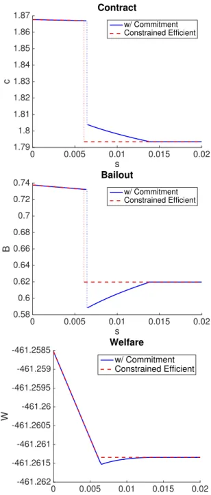
This section includes a numerical example to show the allocation and the wel-fare of the economy under the fiscal authority with commitment. The numerical example uses the following parameter values:

R= 1.5 γ = 1.01 D= 1 y= 3 p= 0.5 τ = 0.5. (1.8)

Figure 1.3 shows the equilibrium allocation and the welfare in the economy under the fiscal authority with commitment and the constrained efficient econ-omy.A = 1.65is such that the constrained efficient allocation falls in Case 2.

The wedge between the blue and red plots in Figure 1.3 shows the range

s∈(s0, s0+k0)in which the economy under the fiscal auhority is not constrained

efficient. Within this range, the fiscal authority realizes that a panic-based run-proof contract is optimal. However, since the bank does not internalize the cost of bailouts, it still prefers to offer a panic-based run-permitting contract. When this happens, the fiscal authority can either allow the bank to offer a panic-based run-permitting contract or lower the bailoutB to incentivize the bank to offer a panic-based run-proof contract. Incentivizing the bank is costly. The fiscal authority has to lower bailout way below the optimal levelB∗ in order for the bank to prefer a panic-based run-proof contract over a run-permitting one (as seen from the Bailout plot in Figure 1.3).

When s is sufficiently close to s0, the fiscal authority still allows the banks

to offer a panic-based run-permitting contract. The cost of incentivizing the bank to offer a panic-based run-proof contract outweighs the cost of tolerating a panic-based run-permitting contract. However, when s gets higher, the cost of tolerating a panic-based run-permitting contract increases. At the same time,

(37)

0 0.005 0.01 0.015 0.02 s 1.79 1.8 1.81 1.82 1.83 1.84 1.85 1.86 1.87 c Contract w/ Commitment Constrained Efficient 0 0.005 0.01 0.015 0.02 s 0.58 0.6 0.62 0.64 0.66 0.68 0.7 0.72 0.74 B Bailout w/ Commitment Constrained Efficient 0 0.005 0.01 0.015 0.02 s -461.262 -461.2615 -461.261 -461.2605 -461.26 -461.2595 -461.259 -461.2585 W Welfare w/ Commitment Constrained Efficient

Figure 1.3: Equilibrium under Fiscal Authority with Commitment (Case 2)

(38)

the cost of incentivizing the bank to offer a panic-based run-proof contract de-creases. Highers forces the bank to be more conservative. The fiscal authority does not have to lower the bailout amount as far below the optimal levelB∗ to incentivize the bank to offer a panic-based run-proof contract. Therefore, as s

gets sufficiently high aboves0, the fiscal authority starts lowering the bailout to

make the bank offer a panic-based run-proof contract. This switch is captured by the discontinuity in the allocation of the economy under the fiscal authority with commitment as seen in Figure 1.3.

Notice that once the fiscal authority decides to lower the bailout to incen-tivize the bank to offer a panic-based run-proof contract, the ex-ante expected welfare is increasing in s. A higher panic-based run probability does not al-ways hurt welfare. Highersinduces banks to behave more conservatively, and consequently decreases moral hazard and increases welfare.

1.5 The Fiscal Authority without Commitment

This section analyzes the economy in which the fiscal authority is unable to pre-commit to a bailout policy. The fiscal authority chooses the bailout policy

B after they observe that both depositors withdraw in period 1. By backward induction, the post-deposit game is first analyzed followed by the pre-deposit game.

(39)

1.5.1 The Post-deposit Game

Taking the deposit contractcas given, the post-deposit game can be solved as an extensive-form game with imperfect information. The fiscal authority observes the withdrawal decisions of the depositors but not sunspots and the types of the depositors. The fiscal authority has to infer sunspots and the types of the depositors from the withdrawal decisions of the depositors.

Each depositor - if patient - has to choose her withdrawal plan for each of the two sunspot states. There are three pure strategies for each depositor: (1) to withdraw late in both statesαandβ, (2) to withdraw late in stateαand early in stateβ, or (3) to withdraw early in both states.21

Definition 5. The separating equilibrium in the post-deposit game under the fiscal authority without commitment is defined as the symmetric separating Perfect Bayesian Equilibrium (PBE) in which both depositors choose action (2).

Definition 6. The “good” (“bad”) pooling equilibrium in the post-deposit game under the fiscal authority without commitment is defined as the symmetric pooling Perfect Bayesian Equilibrium (PBE) in which both depositors choose action (1) ((3)).

The Separating Equilibrium

Suppose both depositors - if patient - choose action (2). When the fiscal author-ity observes that both depositors withdraw early, there is a positive probabilauthor-ity that the second in line is patient. Letpebe the conditional probability of the

sec-ond in line being impatient given that both depositors withdraw early, and is

21_{Without loss of generality, the option for which a patient depositor withdraws early in state} αand late in stateβis omitted.

(40)

given by

e

p= (1−s)p

2₊_sp

(1−s)p2₊_s .

With probability1−s, stateαrealizes and all the patient depositors withdraw late. The probability of both depositors withdrawing early in this state is p2. With probabilitys, stateβrealizes and all depositors withdraw early regardless of their types. The probability of both depositors withdrawing early in this state is 1. In general, the probability of the fiscal authority observing that both depositors withdraw early is(1−s)p2₊_s_{. The probability of the two depositors}

withdrawing early and the second in line being impatient can be derived in a similar way and is given by(1−s)p2+sp.

The bailout decision of the fiscal authority is essentially a trade off between the withdrawal of the second in line and the public good provision. The fiscal authority’s problem is given by

max

B∈[0,2τ y] pue (2(1−τ)y−c+B) + (1−pe)v(2(1−τ)y−c+B) + 2Γ(2τ y−B).

(1.9)

Notice that the utility from the first in line is not in the objective function because the bailout payment is only used to fund the withdrawal of the sec-ond in line. The utility from the public good provision appears in the objective function because the resources for bailouts are taken away from the public good provision.

Let B_sep∗ be the solution to (1.9). The bailout response of the fiscal authority under the assumption that both depositors choose action (2) is given by:

(41)

where Ksep is a constant that is positively correlated with the relative weights

on the utility of the public good provision and the utility of the withdrawal of the second in line ( 2D

e

pA+(1−ep)). Notice that the relative weight is a function of s. Ksepis given by Ksep = ₂_D e pA+(1−ep) 1/γ 1 + 2D e pA+(1−p_e) 1/γ.

Holding the deposit contract c constant, the bailout response of the fiscal authority is negatively correlated with s. As s gets larger, the fiscal authority gets decreasingly certain that the second-in-line depositor is impatient. There-fore, the amount of resources that the fiscal authority intends to reallocate from public goods to the withdrawal of the second in line decreases.

When the value of the public good provision is sufficiently high (Dis large), it could be welfare improving for the fiscal authority to have a negative bailout. This allows the fiscal authority to impose an additional tax on the withdrawal of the second in line to fund the public good. In this case, the non-negativity con-straint for the bailout is binding andB_sep∗ (c) = 0. For the remainder of the paper, the focus is on the parameter values such that the non-negativity constraint for

B_sep∗ (c)is non-binding. This ensures thatB_sep∗ (c)>0.

Lemma 8. Ifγ <min{2,1 + ln 2/lnR}, there exists an interval(csep,¯csep]⊂(0,2(1−

τ)y)such that the separating equilibrium exists in the post-deposit game under the fiscal authority without commitment if and only ifc∈(csep,¯csep].

In order for the fiscal authority’s bailout response B_sep∗ (c) to be such that it is incentive compatible for the depositors to choose action (2), the propensity of the patient depositors to run has to be sufficiently high. This is ensured by

(42)

having a high enough deposit contract csuch that a patient depositor is better off withdrawing early if she believes that the other depositor - if patient - also withdraws early. The propensity to run also has to be low enough such that a patient depositor withdraws late if she believes that the other depositor - if patient - also withdraws late. Lemma 8 suggests that there is a measure of de-posit contract(csep,¯csep] that ensures that both conditions are satisfied and the

separating equilibrium exists in the post-deposit game.

The “Good” and “Bad” Pooling Equilibrium

The “good” pooling equilibrium is when both depositors choose action (1), which is to withdraw late in both statesαand βif they are patient. When both depositors withdraw early, the fiscal authority knows with certainty that the second in line is impatient (pe= 1). The fiscal authority’s problem is given by

max

B∈[0,2τ y]

u(2(1−τ)y−c+B) + 2Γ(2τ y−B). (1.11)

LetB_good∗ be the solution to (1.11). The bailout response of the fiscal authority under the assumption that both depositors choose action (1) is given by

B_good∗ (c) = max{2τ y−Kgood(2y−c),0}, (1.12)

whereKgood is a constant that is positively correlated with the relative weights

on the utility from public good and the utility from the withdrawal of the second-in-line (2_AD). Kgood is given by

Kgood = 2D A 1/γ 1 + 2_AD1/γ .

(43)

The bailout response of the fiscal authority is independent ofssince the de-positors’ actions are independent of the sunspot state. The fiscal authority al-ways knows that the probability of the second in line being impatient is 1.

The analysis of the “bad” pooling equilibrium is similar to the “good” pool-ing equilibrium. When both depositors choose action (3), they withdraw early regardless of their types. Therefore, observing two early withdrawals does not provide the fiscal authority with additional information about the type of the second in line. The conditional probability of the second in line being impatient given two early withdrawals is pe= p, which is equal to the probability of any

given depositor being impatient.

Lemma 9. If γ < min{2,1 + ln 2/lnR}, the “good” (“bad”) pooling equilibrium exists in the post-deposit game under the fiscal authority without commitment as long asc≤csep(c > ¯csep).

To ensure the existence of the “good” pooling equilibrium in the post-deposit game, the best response of the fiscal authority on the bailoutB_good∗ (c) has to be such that it is incentive compatible for the depositors to choose action (1). This happens when the deposit contract c is low (c ≤ csep) so that the propensity

to run of the patient depositors is low enough such that a patient depositor withdraws late if she believes that the other depositor is also withdrawing late. In order for it to be incentive compatible for the depositors to play action (3),

c has to be high enough such that a patient depositor withdraws early if she believes that the other depositor - if patient - also withdraws early. Figure 1.4 provides a summary of the type of equilibrium that exists for a given deposit contractc∈[0,2(1−τ)y].

(44)

0 csep

The “good” pooling equilibrium exists

¯

csep

The separating equilibrium exists

The “bad” pooling equilibrium exists

2(1−τ)y c

Figure 1.4: PBEs of the Post-deposit Game

1.5.2 The Pre-deposit Game

Since the bailout policy is decided by the fiscal authority later on when both depositors in a bank withdraw in period 1, the bank knows that the deposit contract it offers affects the decision of the fiscal authority on the amount of bailout. It is clear from the response functions of the fiscal authority in (1.10) and (1.12) that the bailout response is an increasing function ofc. The bank does not internalize the cost of bailouts but is able to indirectly increase the bailout amount by increasingc. This is the driving force of moral hazard that arises due to the lack of commitment of the fiscal authority in this model.

The bank knows that the choice of its deposit contract dictates the type of equilibrium in the post-deposit game based on Lemma 8 and 9. The representa-tive bank’s problem is given by

max c∈[0,¯csep]        c

Wpri(c, Bgood∗ (c)) ifc≤csep

f

Wpri(c, Bsep∗ (c);s) ifc >csep

. (1.13)

The bank only maximizes the ex-ante expected utilities of its own depositors from withdrawalsWpridue to the competitive nature of the banking industry.

(45)

c

Wpri(c, Bgood∗ (c))is the sum of the ex-ante expected utilities from withdrawals

of the two depositors when there is the “good” pooling equilibrium in the post-deposit game.Wf_pri(c, B_sep∗ (c);s)is the sum of the ex-ante expected utilities from

withdrawals of the two depositors when there is the separating equilibrium in the post-deposit game. Letc∗₂ denote the solution to (1.13).22 _{The full} equilib-rium characterization can be found in Section A.5 of the Appendix.

Proposition 10. The economy in which the fiscal authority is unable to commit is never constrained efficient.

The main takeaway from Proposition 10 is that the inability of the fiscal au-thority to commit to a bailout policy is the main driving force of the moral haz-ard in the banking industry. If the fiscal authority is able to commit, the outcome is typically constrained efficient (Proposition 7). The disparity between the com-mitment case and the non-comcom-mitment case is mainly due to the failure of the bank to internalize the cost of bailouts and the ability of the bank to indirectly affect the bailout it receives by altering the deposit contract it offers.

1.5.3 Numerical Example

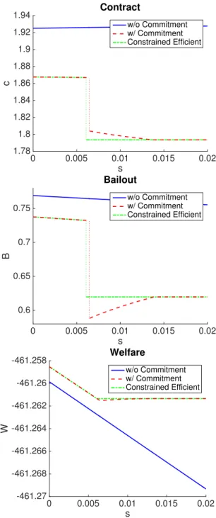
The same parameter values from (1.8) are used. Figure 1.5 shows the equi-librium outcome in the non-commitment case together with the equiequi-librium

22_{There exists a range}_c_∈₍_c

good,csep]such that it is incentive compatible for the depositors to

both choose action (1) or both choose action (3). Choosing action (1) in both sunspot states can still be supported as an equilibrium. However, it does not give a fair comparison between the commitment and non-commitment case. This is because in the commitment case, the depositors are assumed to always play the non-panic equilibrium inαstate and panic equilibrium inβstate whenever both equilibria exist. The focus of the parameter values for the remainder of the paper is such thatc∗₂ ∈/ (cgood,csep]. The detail on the parameter restrictions can be found in Section

(46)

outcomes in the commitment case and the constrained efficient economy when

A= 1.65. The plots of the contract, bailout, and welfare for the non-commitment case and the constrained efficient economy are identical to Figure 1.3. For the entire measure ofsshown in Figure 1.5, the separating equilibrium exists in the post-deposit game under the fiscal authority without commitment.

Notice that the deposit contractcis higher under the fiscal authority without commitment than the one under the fiscal authority with commitment and the one in the constrained efficient economy. This is due to the bank’s expectation that the fiscal authority will increase bailoutB if it offers a higher deposit con-tractc. In equilibrium, bailoutBunder the fiscal authority without commitment is also higher than the ones in the other two economies. The ex-ante expected welfare under the fiscal authority without commitment is strictly lower than the constrained efficient welfare and the welfare under the fiscal authority with commitment.

The Cost of Non-commitment

In order to better illustrate the cost of moral hazard under the fiscal authority with and without commitment, the amounts of additional endowments on top ofy that are required to bring the equilibrium welfare under both cases to the constrained efficient welfare are computed. Define∆C_y and∆N C_y respectively as the corresponding amounts of additional endowments required for each depos-itor in the commitment and non-commitment case. The difference∆N C

y −∆Cy is

the cost of the inability of the fiscal authority to commit. Figure 1.6 shows the plot of∆C

(47)

0 0.005 0.01 0.015 0.02 s 1.78 1.8 1.82 1.84 1.86 1.88 1.9 1.92 1.94 c Contract w/o Commitment w/ Commitment Constrained Efficient 0 0.005 0.01 0.015 0.02 s 0.6 0.65 0.7 0.75 B Bailout w/o Commitment w/ Commitment Constrained Efficient 0 0.005 0.01 0.015 0.02 s -461.27 -461.268 -461.266 -461.264 -461.262 -461.26 -461.258 W Welfare w/o Commitment w/ Commitment Constrained Efficient

(48)

0 0.005 0.01 0.015 0.02 s 0 1 2 3 4 5 6 ∆ y

×10-3 Compensation to get to CEA

w/o Commitment w/ Commitment

Figure 1.6:

from (1.8) andA = 1.65. Notice that ∆C

y is relatively close to or equal to zero

for the entire measure of s. When the fiscal authority is able to commit, the moral hazard cost is minimal. Also,∆N C

y is strictly increasing ins. As the

panic-based run probability gets larger, the moral hazard cost of the inability of the fiscal authority to commit increases. For small s, ∆C_y is less responsive to an increase ins. This is because constrained efficient contract is panic-based run-permitting while the non-commitment case has the separating equilibrium in the post-deposit game. In equilibrium, the depositors play the same strategies in the post-deposit game in both economies. As s gets larger, the constrained efficient contract switches to panic-based run-proof but the non-commitment case still has the separating equilibrium in the post-deposit game. The deposi-tors play a different strategy in each economy. The constrained efficient welfare is constant insbut the welfare in the non-commitment case is strictly decreasing ins. Therefore,∆N C

(49)

1.6 Controlling Short-term Interest Rates

This section evaluates the efficacy of an additional policy tool for the fiscal au-thority in eliminating the moral hazard from bailouts.

Since banks tend to offer a deposit contractchigher than the efficient level, it can be welfare improving if the fiscal authority is able to place an upper bound on the contract offered by banks.23 _{The fiscal authority chooses an upper bound} on the deposit contract¯cright after taxes are collected.

Proposition 11. Suppose the fiscal authority is able to place an upper bound on con-tracts. When the fiscal authority is able to commit, the economy is always constrained efficient. When the fiscal authority is unable to commit, the economy is constrained efficient ifs ∈ [0,s¯), where s¯ = 1 if the constrained efficient allocation is in Case 1, ¯

s∈(0, s0]in Case 2, ands¯= 0in Case 3.

When the fiscal authority is able to commit, the optimal choices for bailout and the upper bound for contracts are trivial. The fiscal authority chooses

B = B∗ and ¯c = c∗.24 _{The upper bound for contracts is binding and the bank} choosesc∗. In equilibrium, the allocation is identical to the constrained efficient allocation. The economy is constrained efficient fors ∈[0,1].

When the fiscal authority is unable to commit, the optimal choice for¯cis less trivial. Assuming that the fiscal authority chooses the deposit contract on behalf

23_{Contract is essentially the short-term interest rate offered by the bank. The short-term rate}

can be calculated by c (1−τ)y.

(50)

of the bank, the fiscal authority’s problem is given by

c∗_optimal ≡arg max

c∈[0,c¯sep]        c W(c, B_good∗ (c)) ifc≤csep f W(c, B_sep∗ (c);s) ifc >csep . (1.14)

(1.14) differs from (1.13) and in that the ex-ante expected welfare is max-imized in (1.14) but only the ex-ante expected utilities from withdrawals are maximized in (1.13). The contract c∗_optimal chosen by the fiscal authority gives the highest possible welfare in the non-commitment case. Naturally, the fiscal authority’s optimal choice for the upper bound isc¯=c∗_optimal.25

WhenA ≤Aearly (Case 1), the constrained efficient allocation is(_bc,Bb)and is

panic-based run-proof fors ∈ [0,1]. The solution to (1.14) is also bc. The fiscal

authority’s optimal upper bound for contracts is¯c=_bc. Since the bank typically chooses a deposit contract that is higher than the constrained efficient level, the upper bound is strictly binding. The bank’s optimal deposit contract isbc, which

gives the “good” equilibrium in the post-deposit game. The fiscal authority’s bailout response in the post-deposit game is B_good∗ (_bc) = Bb. The equilibrium

allocation turns out to be(_bc,Bb), which is identical to the constrained efficient

allocation. Therefore, the economy is constrained efficient fors∈[0,1].

When Aearly _{< A} _≤ _Await _{(Case 2), the constrained efficient allocation is}

(_ec,Be)and is panic-based run-permitting fors ∈[0, s₀). It can be shown that the

solution to (1.14) is also ec fors ∈ [0,s¯). The fiscal authority then chooses ec as

the upper bound and the bank responds with_ecsince the upper bound is strictly binding, as shown in Figure 1.5. The equilibrium allocation is (_ec,Be), which is

identical to the constrained efficient allocation. Therefore, the economy is

con-25_{It remains to check that when}_c_¯₌ _c∗

optimal, the bank responds by choosingc∗optimal. That

ensures that the optimal upper bound of the fiscal authority is¯c=c∗ optimal