Robustifying Binary Classification to Adversarial Perturbation
Fariborz Salehi and Babak Hassibi
Abstract— Despite the enormous success of machine learning models in various applications, most of these models lack resilience to (even small) perturbations in their input data. Hence, new methods to robustify machine learning models seem very essential. To this end, in this paper we consider the problem of binary classification with adversarial perturbations. Investigating the solution to a min-max optimization (which considers the worst-case loss in the presence of adversarial perturbations) we introduce a generalization to the max-margin classifier which takes into account the power of the adversary in manipulating the data. We refer to this classifier as the "Robust Max-margin" (RM) classifier. Under some mild assumptions on the loss function, we theoretically show that the gradient descent iterates (with sufficiently small step size) converge to the RM classifier in its direction. Therefore, the RM classifier can be studied to compute various performance measures (e.g. generalization error) of binary classification with adversarial perturbations.
I. INTRODUCTION
Machine learning models have been very successful in many applications, ranging from spam detection, speech and visual recognition, to the analysis of genome sequencing and financial markets. Yet, despite this indisputable success, it has been observed that commonly used machine learning models (such as deep neural networks) are very instable in the presence of non-random perturbations [16], [1], [2].
The instability of machine learning models is a fun-damental issue that needs to be addressed, especially when such models are used in sensitive applications such as autonomous systems. There have been many recent efforts to address this issue (a partial list of papers includes [9], [19], [13].) However, robustness comes at a cost and it is often the case that the adversarial training al-gorithms underperform on the clean data when compared with their (non-robust) counterparts. Understanding the tradeoffs (in accuracy) between the robust and standard models is an important problem the answer to which can help us find more efficient training methods. Recently, Javanmard et. al. [7] precisely characterized the tradeoff between standard and adversarial risks for the linear regression problem. They also analyze the performance F. Salehi and B. Hassibi are with the Department of Electrical Engineering, California Institute of Technology, Pasadena, CA 91125, USA. {fsalehi, hassibi}@caltech.edu
of the resulting model under i.i.d. Gaussian training data. In this paper, we study the simple (yet fundamental) problem of binary classification where the goal is to find a classifier that has a high accuracy in predicting the binary labels when having feature vectors as its input. When the clean data is available, max-margin classifier [18] is the model of choice as maximizing the margin is interpreted as minimizing the risk of misclassification [3]. Recently, it was shownin [14] that for a broad class of loss functions, including the well-known logistic loss, the gradient descent iterates converge to the max-margin classifier. More recently, the asymptotic performance of this classifier has been characterized in [10], [4], [12]. We consider the case where the training data is perturbed by an adversary and introduce the "Robust Max-margin" (RM) classifier as a generalization of max-margin to perturbed input data. We then consider the adversarial training method, in which the optimal parameter is a solution to a saddle-point optimization. We show that the gradient descent algorithm with properly-tuned step sizes converges in its direction to the RM classifier. A significant consequence of this result is that one can characterize various performance measures (e.g. generalization error) of adversarial training in binary classification by analyzing the performance of the RM classifier.
To the extent of our knowledge, this is the first work that introduces the robust max-margin classifier and proves the convergence of gradient descent iterates to this classifier. This paper was originally submitted on March2020to the Conference on Decision and Control (CDC). We should note that more recently in [6], the authors have shown similar results (referred to as the "robust separation") and analyze the performance of the resulting classifier under i.i.d. Gaussian training data. Their analysis on the performance of the resulting estimator is based on the Convex Gaussian Min-max Theorem [15], [17]. Similar analyses have been recently provided for the performance of max-margin classifiers as well as other generalized linear models [11], [10], [4], [5], [12].
The organization of the paper is as follows: In Section II we provide some background on the binary classification problem and how it connects with the max-margin
classifier. The mathematical setup for the problem of binary classification with perturbed training data is provided in Section III. The main result of the paper is presented in Section IV, and the proofs are provided in Sections V and VI.
II. PRELIMINARIES A. Notations
For any vectorw∈Rp, the binary classifier associated
with w is defined as: Cw : Rp → {±1}, such that
Cw(x) =Sign(wTx).Ndenotes the set of non-negative
integers. For a vectorv,vT denotes its transpose, and
kvkp (forp≥1) is its`p norm, where we often omit
the subscript forp= 2.σmax(M)denotes the maximum singular value of the matrix M.0d and1d respectively
represent the all-one and all-zero vectors in dimensiond. A function f(·)is said to beL-smooth if its derivative,
f0(·), isL-Lipschitz.
B. Background: binary classification with unperturbed data
Let D={(xi, yi) : 1≤i≤n} denote a set of data
points, where fori = 1, . . . , n, xi ∈Rp is the feature
vector, andyi ∈ {±1} is the binary label. We assume
that D is linearly separable, i.e., there exist w? ∈
Rp
such that:
yi =Sign(xTiw
?), for i= 1,2, . . . , n. (1)
When the training data has no perturbation, one can attempt to find a classifier by minimizing the empirical loss on datasetD. In the setting of binary classification, the loss function is usually formed as,
L(w) =
n
X
i=1
`(yixTi w) (2)
where the function `(·) : R → R+ is a decreasing function that approaches0as its input approaches infinity. A typical approach to find the minimizer of the loss functionL(w)is through the iterative algorithms, such as the gradient descent (GD) algorithm. The convergence of the GD iterates on separable datasets has been studied in recent papers [8], [14], where it was shown, among others, that while the norm of the iterates approaches infinity, their direction would approach to the direction of the well-knownL2 max-margin classifier defined as,
wM = arg min
w∈Rp
kwk
s.t. yixTi w≥1 , 1≤i≤n.
(3) In other words, their result states that for almost every x ∈ Rp, Cwt(x) → CwM(x) as t grows, where wt denotes the result of GD after tsteps. The max-margin
classifier (3) (a.k.a. hard-margin SVM [3]) has been extensively studied in the machine learning community. This classifier simply maximizes the smallest distance of the data points to the separating hyperplane (referred to as the margin).
The abovementioned result, i.e., convergence of the GD iterates to the max-margin classifier, has significant consequences as the max-margin classifier can then be studied to compute various performance measures (such as the generalization error) of the resulting estimator. Very recently, researchers have exploited this result to accurately compute the generalization error of GD over the logistic loss [10].
III. BINARY CLASSFICATION WITH ADVERSARIAL PERTURBATION
As explained earlier in Section I, understanding the behavior of machine learning models under perturbed input is very essential with the goal of improving the robustness of these models. Inspired by recent advances in understanding the behavior of machine learning models under adversarial perturbation, here we study the problem of binary classification with perturbed data.
We assume that the training data is a perturbed version of the underlying dataset,D. Let D0={(x
i+zi, yi) :
1≤i≤n} denote the set of training data, where, for
i= 1,2, . . . , n,zi∈ Siis the unknown perturbation, and
the setSi consists of all the allowed perturbation vector.
In the adversarial setting it is often assumed that the perturbation vectors,{zi}ni=1, are chosen in such a way that the training algorithm is beguiled into generating a wrong solution.
Throughout this paper, we assume that the perturbation vectors have bounded norms by defining Si = iBp,
where Bp denotes the unit ball inRp, andi ≥0, for
1 ≤ i ≤n, indicates the maximum allowed norm for thei-th perturbation vector,zi. While the perturbation
vectors are hidden to us, we assume having knowledge of{i}ni=1.
Note that the set of allowed perturbations can be different for different data points. This includes certain special cases such as: (1) only a subset of the data is perturbed (i = 0if the i-th data point is not perturbed), and (2)
all the data points have the same perturbation set, i.e., for some≥0 we have i= for1≤i≤n, .
A. Saddle-point optimization
The parameters of the desired model are often derived by forming a loss function and solving an optimization problem to find a minimizer of the loss. In adversarial training, one should also consider the manipulative power of the adversary where the adversary attempts to misguide
the training algorithm. When the goal of a training algorithm is to minimize a loss function, one can view the adversary as an entity which attempts to maximize the loss. The followingmin-maxoptimization problem incorporates the contrary behaviors of the adversary and the training algorithm with respect to the loss function.
min w∈Rp max zi∈Si,1≤i≤n L(w) := n X i=1 ` yi(xi+zi)Tw . (4) In order to find a robust model, we should solve this saddle-point optimization. Under our assumptions on the perturbation sets, we can introduce the functionL(w) which is the result of the inner maximization in (4), i.e.,
L(w) = n X i=1 max kzik≤i ` yi(xi+zi)Tw , (5)
where= [1, 2, . . . , n]T. Therefore, the robust
classi-fier is defined as a minimizer ofL(w). IV. MAINRESULTS
In this section, we present the main results of the paper. First, in Section IV-A we introduce the Robust
Max-margin (RM) classifier as an extension of the max-margin classifier when the training data is perturbed. Consequently, in Section IV-B, we show that, under some conditions on the function `(·), gradient descent algorithm (with sufficiently small step size) would converge in its direction to the RM classifier.
A. Robust Max-margin (RM) Classifier
The max-margin classifier is a classifier that maximizes the minimum distance of the data points to the separating hyperplane (margin). In our setting where the training data is perturbed we should modify the notion of the margin to incorporate various perturbations across data points. More specifically, in order to get a robust classifier we would like the data points with higher perturbations to be farther away from the resulting separating hyperplane.
TheRobust Max-margin classifier is defined as, w(RM) := arg min
w∈Rp
kwk
s.t. yixTi w≥1 +ikwk , 1≤i≤n.
(6) As observed in the constraints of this optimization, the RM classifier enforces data points with higher perturbations to keep a larger distance from the separating hyperplane {x:wTMx= 0}.
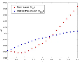
When the data is perturbed, we expect the RM classi-fier to outperform the max-margin classiclassi-fier. Figure 1 depicts a comparison in generalization error between the
Fig. 1: A comparison in generalization error (GE) be-tween the max-margin (3) and the robust max-margin (6). The result is the average over 20 independent trials with n = 100 and p = 40. The data is generated from a Gaussian distribution and 40% of data points are perturbed with maximum norm of. For large values of, the RM classifier has a better generalization error than the max-margin classifier.
max-margin and the RM classifier. Although for small perturbations, the two model behave the same, the RM classifier has a better performance as we increase the norm of perturbations.
While the separability of the data is necessary for the existence of the RM classifier, it is not sufficient. The following lemma provides a sufficient condition for its existence.
Lemma 1: The RM classifier exists when the data set
D={(xi, yi) : 1≤i≤n}is separable and,
kk∞< 1
kwMk2
, (7)
wherewM is the max-margin classifier.
Proof: The max-margin classifer,wM, exists when
Dis linearly separable. Also,w¯ = 1 1−kk∞kwMk2
wM is
a feasible point of the optimization (6). Therefore, the RM classifier exists andkwMk ≤ kwRMk ≤ kw¯k.
When the perturbation sets are the same for different data points, one expects the RM classifier to be the same as the max-margin classifier.
Lemma 2: If = ×1n for some ≥ 0, the RM
classifier exists if and only if <kw1
Mk. In this case, wRM =
wM
1−kwMk
Proof: Assume wRM exists, then we have w¯ =
wRM
1+kwRMksatisfies the constraints in the optimization (3). SincewM is the solution to this optimization, we have
kwMk ≤ kw¯k which gives · kwMk < 1. It is easy
to check that w = wM
1−kwMk is the solution to the optimization (6), as it satisfies the constraints and wM
is the optimal value of the optimization program (3). B. Convergence of GD Iterates
In this section, we present the main result of the paper that is the convergence of the gradient descent iterates to the RM classifier. As discussed earlier in Section III-A, the goal is to solve the following optimization problem.
min
w∈Rp
L(w), (9)
where L(·)is defined in (5). Gradient descent (GD) is the common method of choice to find a minimizer of this optimization. Starting from an initialization,w0∈
Rp, the GD iterates are generated through the following
update rule:
wt+1 =wt−η· ∇L(wt), for t∈N, (10)
whereη >0 is the step size.
Our goal is to study the behavior of the GD iterates ast
grows large. For our analysis, we need some assumptions to hold for the loss function`(·).
Assumption 1: The function ` : R → R+ is twice-differentiable, monotonically decreasing, andβ-smooth. We note that the common choices of the loss function satisfy the conditions in Assumption 1. For instance, the logistic loss defined as `(u) = log 1 + exp(−u) satisfies these conditions (withβ = 1.) We first state the following lemma which provides some insights on the behavior of GD iterates,wt, ast→ ∞.
Lemma 3: Consider the gradient descent iterates (10) with step size η <2·β−1·(σ
max(X) +kk)−2, where X = [x1,x2, . . . ,xn]T ∈ Rn×p is the data matrix, L is defined in (5), and`(·)satisfies Assumption 1. If the RM classifier exists, then, ast→+∞we have,
i. kwtk →+∞,
ii. ∇L(wt)→0p , and,
iii. yixTiwt−ikwtk →+∞, for i= 1,2, . . . , n.
The proof of this lemma is provided in Section V. Lemma 3 provides useful insights on the behavior of the gradient descent iterates. With small enough step size, ast
grows the norm ofwtbecomes unbounded while making
L(wt)closer to zero. Sincewt diverges, we focus our
attention on its direction, i.e., the normalized vector
wt
kwtk. In fact, the classifier defined bywt,Cwt(·), only depends on its direction. Therefore, if wt
kwtk converges, we can claim that the classifiers generated by GD iterates
converge.
Our main result in Theorem 1 states that the classifiers generated form the GD iterates converges to the RM classifier defined in Section IV-A. Before stating this result, we need the following definition which is a modified version of an assumption in [14].
Definition 1: A functionf(u)has a tight exponential tail if there exist positive constants a, c, τ, µsuch that for allu > τ:
(
f(u)≤c 1 + exp(−µ·u)exp(−a·u), and, f(u)≥c 1−exp(−µ·u)
exp(−a·u).
(11) Theorem 1: Let Assumption 1 holds and −`0(·) has a exponential tail. Consider the gradient descent iterates in (10) withη <2·β−1·(σ
max(X) +kk)−2. Then, for almost every dataset we have,
lim t→∞ wt kwtk − wRM kwRMk = 0. (12)
Threfore, the resulting classifier converges to the RM classifier.
Remark 1: The assumption on −`0(·)having a tight exponential tail holds for common loss functions in binary classification. As an example, the derivative of the logistic function satisfies (11) witha=c=µ= 1.
Remark 2: Theorem 1 states that whilewtdiverges
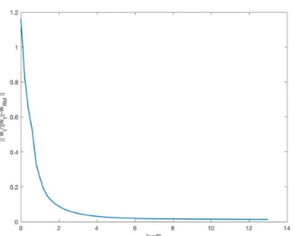
as t grows , its direction converges to the direction of the robust max-margin classifier. We should note that this convergence is quite slow. Figure 2 depicts the convergence of the direction of GD iterates to the RM classifier ast→ ∞where it can be observed the convergence becomes slow as t grows (the horizontal axis has a logarithmic scale.) In our proof in Section VI we theoretically stablish that the rate of convergence is logarithmic.
V. PROOF OFLEMMA3
In our proof we use the following lemma which characterizes the behavior of gradient descent iterates on smooth functions.
Lemma 4 (Lemma 10 in [14]): Let L(w) be a γ -smooth non-negative objective. Ifη < 2γ, then, for any starting pointw(0), with the GD sequence
w(t+ 1) =w(t)−η∇L(w(t)) we have that: ∞ X u=0 k∇L(w(u))k2<+∞.
Fig. 2: Convergence of GD iterates to the RM classifier. For our experiment we have n= 30, p= 10, number of iterations is 1013, and
i ∼ Unif(0,kw1
Mk). The distance between the max-margin and the RM classifier is wM kwMk − wRM kwRMk = 0.2192.
Corollary 1: For any positive constant C < β σmax(X) +kk
2
, there exist R > 0, such that
∇2L(w)
< C whenkwk> R.
The proof is straightforward, by computing the Hessian ofL(·)and using the fact that`(·)is twice-differentiable andβ-smooth.
Since the function `(·) is monotonically decreasing we can write, L(w) = n X i=1 `(yixTiw−ikwk) (13)
The gradient of the loss function can be computed as,
∇L(w) = n X i=1 `0(yixTiw−ikwk)(yixi−i w kwk). (14) Consider the sequence st := 1ηwRMT wt, for t ∈ N.
First, we show that this sequence is increasing.
st−st+1=wTRM∇L(wt) (15) = n X i=1 `0(yixTiwt−ikwtk)wTRM yixi−i wt kwtk ≤ n X i=1 `0(yixTiwt−ikwtk) yixTiwRM −ikwRMk ≤ n X i=1 `0(yixTiwt−ikwtk)<0 ,
where for the first inequality we used the fact that
`0(u) < 0 and Cauchy-Schwartz, and for the second
inequality we used the constraints of the optimization (6). Since{st}t≥0 is an increasing sequence inR it either
grows to+∞or approaches a limit value. We analyze each of these cases separately.
Case 1: lim
t→∞st=L <+∞
When the sequence has a limit, we have limt→∞st−st+1 = 0. From the last inequality in (15), this implies that ast→ ∞,
`0(yixTi wt−ikwtk)→0, for 1≤i≤n. (16)
Since`0(u)is negative foru∈
R, we must have
yixTi wt−ikwtk →+∞, for1≤i≤n, (17)
which is (iii). This also implies that kwtk → ∞.
Finally, from (14) we have that ∇L(wt) → 0p.
Case 2: lim
t→∞st= +∞ kwtk ≥ kwηst
RMk implies that limt→∞kwtk = +∞. Using Corollary 1, for any constantC < β σmax(X) +
kk2
, there exists a nonnegative integer t0 such that the second derivative is bounded by C for any t > t0. Hence, we can use the result of Lemma 4 with η <
2·β−1·(σ
max(X)+kk)−2which givesk∇L(wt)k →0
ast→+∞.
In order to show (iii), we use the last inequality in (15), ast→ ∞sincewTRM∇L(wt)→0, we have:
`0(yixTi wt−ikwtk)→0, for 1≤i≤n, (18)
which gives the desired result.
VI. PROOF OFTHEOREM1
For the RM classifier, we define the set of support vectors as:
S=SRM :={i∈[n] :yixTi wRM = 1 +ikwRMk},
(19) First, we consider the KKT conditions for the optimiza-tion (6) which gives:
wRM = X i∈S αi yixi−iwˆ , (20) where wˆ := wRM
kwRMk and αi ≥ 0. It can be shown that when the data points are drawn from a continuous distribution, for almost every dataset the support vectors are linearly independent andαi’s are all positive (see
also [8] and Appendix B in [14]). Given the fact that
−`0(u)has a exponential tail, we assume α, γ, τ, µare positive constants such that:
( −`0(u)≤γ 1 + exp(−µ·u) exp(−α·u), and, −`0(u)≥γ 1−exp(−µ·u) exp(−α·u), (21)
for everyu≥τ.
We define a vectorw˜ such that: exp ˜wT(yixi−iw)ˆ
:= αi
γ·η , for i= 1,2, . . . , n.
(22) Recall that the gradient descent iterates are defined as,
wt+1−wt=−η∇L wt
, t∈N. (23)
Next, fort≥0we define the residual vectorrt∈Rp.
rt:=wt−
1
αlog(t)wRM−w˜. (24)
In our proof, we adopt a similar strategy as [14] and bound the norm of the residual vector kr(t)k by a constant C for every t ≥ 1. Consider the following equation, krt+1k 2 − krtk 2 =krt+1−rtk 2 + 2 rTt rt+1−rt . (25) We bound each of the two terms in the RHS of (25). We start with bounding the first term in the (25). We have:
krt+1−rtk 2 = wt+1−wt−wRM log( t+ 1 t )/α 2 ≤η2k∇L(wt)k 2 + (αt)−2kwRMk 2 + 2(η/α) log(1 +t−1)wRMT∇L(wt) ≤η2k∇L(wt)k 2 + (αt)−2kwRMk 2 . (26) Where in the first inequality we replaced wt+1−wt
using the gradient descent iterates (23) along withlog(1+
u)≤u, and in the second inequality we exploited the inequality (15) that giveswˆT∇L(w(t))<0.
Since the norm ofwt approaches infinity astgrows,
when η <2·β−1·(σmax(X) +kk)−2we can use the result of Corollary 1 and Lemma 4 to have:
∞
X
t=0
k∇L(wt)k< C1, (27)
for some constantC1>0. Therefore, we can bound the sum over the first term in (25).
X t≥1 ||rt+1−rt||2≤η2C1+α−2kwRMk2 X t≥1 t−2< C2. (28) Next, we will bound the second term in (25), i.e., rT
t rt+1−rt
. To do so, we first define the constant θ
as follows:
θ:= min
i∈ScyixiwRM−ikwRMk>1, (29) whereSc = [n]− S indicates the indices of non-support
vectors. The following lemma provides an upper bound onrT
t rt+1−rt
fort≥1.
Lemma 5: With the assumptions of Theorem 1, con-sider the gradient descent iterates (23), {wt}t∈N, and the vectorrt defined in (24). Then, for constantsC≥0
andt0∈N, we have:
rTt rt+1−rt
≤Ct−min(θ,1+2µα) , ∀t≥t0. (30) Using the result of Lemma 5, sinceθ >1and µ/α >0 we have: X t≥0 rTt rt+1−rt< t0−1 X t=1 rTt rt+1−rt+C X t≥t0 t−min(θ,1+2µα) < C3. (31) Therefore, from (25), (28), and (31), we have,
krkk2=kr1k2+ k−1 X t=1 krt+1k2− krtk2< C4, ∀k≥1. (32) for a positive constantC4. Consequently, from (24) we have, wt− 1 αlog(t)wRM ≤C4+kw˜k, (33)
By some straightforward calculations we can get, wt kwtk − wRM kwRMk 2 ≤2α(C4+kw˜k) log(t)kwRMk 2 , (34) which gives the desired result, i.e.,
lim t→∞ wt kwtk − wRM kwRMk = 0. (35) REFERENCES
[1] Battista Biggio, Igino Corona, Davide Maiorca, Blaine Nelson, Nedim Srndi´c, Pavel Laskov, Giorgio Giacinto, and Fabio Roli. Evasion attacks against machine learning at test time. In Joint European conference on machine learning and knowledge discovery in databases, pages 387–402. Springer, 2013. [2] Nicholas Carlini and David Wagner. Towards evaluating the
robustness of neural networks. In 2017 ieee symposium on security and privacy (sp), pages 39–57. IEEE, 2017.
[3] Corinna Cortes and Vladimir Vapnik. Support-vector networks. Machine learning, 20(3):273–297, 1995.
[4] Zeyu Deng, Abla Kammoun, and Christos Thrampoulidis. A model of double descent for high-dimensional binary linear classification. arXiv preprint arXiv:1911.05822, 2019. [5] Melikasadat Emami, Mojtaba Sahraee-Ardakan, Parthe Pandit,
Sundeep Rangan, and Alyson K Fletcher. Generalization error of generalized linear models in high dimensions. arXiv preprint arXiv:2005.00180, 2020.
[6] Adel Javanmard and Mahdi Soltanolkotabi. Precise statistical analysis of classification accuracies for adversarial training.arXiv preprint arXiv:2010.11213, 2020.
[7] Adel Javanmard, Mahdi Soltanolkotabi, and Hamed Hassani. Precise tradeoffs in adversarial training for linear regression. arXiv preprint arXiv:2002.10477, 2020.
[8] Ziwei Ji and Matus Telgarsky. Risk and parameter convergence of logistic regression. arXiv preprint arXiv:1803.07300, 2018.
[9] Aleksander Madry, Aleksandar Makelov, Ludwig Schmidt, Dim-itris Tsipras, and Adrian Vladu. Towards deep learning models resistant to adversarial attacks. arXiv preprint arXiv:1706.06083, 2017.
[10] Andrea Montanari, Feng Ruan, Youngtak Sohn, and Jun Yan. The generalization error of max-margin linear classifiers: High-dimensional asymptotics in the overparametrized regime. arXiv preprint arXiv:1911.01544, 2019.
[11] Fariborz Salehi, Ehsan Abbasi, and Babak Hassibi. The impact of regularization on high-dimensional logistic regression. In Advances in Neural Information Processing Systems, pages 11982– 11992, 2019.
[12] Fariborz Salehi, Ehsan Abbasi, and Babak Hassibi. The per-formance analysis of generalized margin maximizer (gmm) on separable data. International Conference on Machine Learning (ICML), 2020.
[13] Ali Shafahi, Mahyar Najibi, Mohammad Amin Ghiasi, Zheng Xu, John Dickerson, Christoph Studer, Larry S Davis, Gavin Taylor, and Tom Goldstein. Adversarial training for free! InAdvances in Neural Information Processing Systems, pages 3353–3364, 2019. [14] Daniel Soudry, Elad Hoffer, Mor Shpigel Nacson, Suriya Gu-nasekar, and Nathan Srebro. The implicit bias of gradient descent on separable data. The Journal of Machine Learning Research, 19(1):2822–2878, 2018.
[15] Mihailo Stojnic. A framework to characterize performance of lasso algorithms. arXiv preprint arXiv:1303.7291, 2013. [16] Christian Szegedy, Wojciech Zaremba, Ilya Sutskever, Joan Bruna,
Dumitru Erhan, Ian Goodfellow, and Rob Fergus. Intriguing properties of neural networks. arXiv preprint arXiv:1312.6199, 2013.
[17] Christos Thrampoulidis, Samet Oymak, and Babak Hassibi. Regularized linear regression: A precise analysis of the estimation error. InConference on Learning Theory, pages 1683–1709, 2015. [18] V Vapnik. Estimation of dependences based on empirical data
berlin, 1982.
[19] Weilin Xu, David Evans, and Yanjun Qi. Feature squeezing: Detecting adversarial examples in deep neural networks. arXiv preprint arXiv:1704.01155, 2017.