City University of New York (CUNY)
CUNY Academic Works
School of Arts & Sciences Theses Hunter College
Spring 5-19-2016
Exploring Data Mining Techniques for Tree
Species Classification Using Co-Registered LiDAR
and Hyperspectral Data
Julia K. Marrs
CUNY Hunter College
How does access to this work benefit you? Let us know!
Follow this and additional works at:http://academicworks.cuny.edu/hc_sas_etds
Part of theDatabases and Information Systems Commons,Numerical Analysis and Scientific Computing Commons, and theOther Forestry and Forest Sciences Commons
This Thesis is brought to you for free and open access by the Hunter College at CUNY Academic Works. It has been accepted for inclusion in School of Arts & Sciences Theses by an authorized administrator of CUNY Academic Works. For more information, please [email protected]. Recommended Citation
Marrs, Julia K., "Exploring Data Mining Techniques for Tree Species Classification Using Co-Registered LiDAR and Hyperspectral Data" (2016).CUNY Academic Works.
1
Exploring Data Mining Techniques for Tree Species Classification Using Co-Registered LiDAR and Hyperspectral Data
by Julia Marrs
Submitted in partial fulfillment of the requirements for the degree of
Master of Arts in Geography Hunter College of the City of New York
2016
Thesis Sponsor:
05/19/2016 Dr. Wenge Ni-Meister
Date First Reader
05/19/2016 Dr. Carsten Kessler
2
Table of Contents Page
Abstract Introduction 3 4 Methods 20 Results 33 Discussion 42 Appendix 47 Bibliography 52
List of Figures Page
Figure 1: Layout of Subplots Within Whole Plots 24
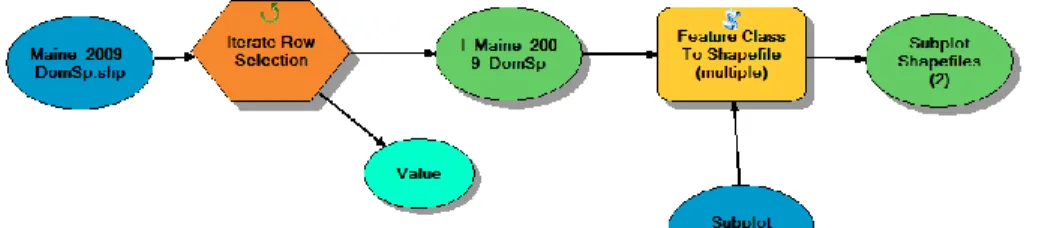
Figure 2: ModelBuilder Tool for Exporting Rows as Individual Shapefiles 26
Figure 3: Sample Orange Workflow for Comparing Data Mining Methods 29
Figure 4: Sample Classification Tree Workflow 32
Figure 5: Sample Simplified Orange Workflow 33
Figure 6: Plots of Individual Tree Diameter at Breast Heights by Species 35
Figure 7: Comparison of Resampling Techniques and Data Mining Methods Using Complete Lists of Metrics
37 Figure 8: Comparison of Resampling Techniques and Data Mining Methods Using
Simplified and Generic Lists of Metrics
40
List of Tables Page
Table 1: List of LiDAR Metrics and Abbreviations 21
Table 2: Select List of Hyperspectral Vegetative Indices and Abbreviations 23
Table 3: Tree Species Abbreviations 25
Table 4: Justification For Resolving Dominant Species Ties in Four Subplots 26
3 Abstract
The use of LiDAR techniques for recording and analyzing tree and forest structural variables shows strong promise for improving established hyperspectral-based tree species classifications, but previous multi-sensoral projects have often been limited by error resulting from seasonal or flight path differences. NASA Goddard’s LiDAR, Hyperspectral, and Thermal imager is now providing co-registered data on experimental forests in the United States, which are associated with established ground truths from existing forest plots. Free, user-friendly data mining applications like the Orange Data Mining Extension for Python have recently simplified the process of combining datasets, handling variable redundancy and noise, and reducing dimensionality in remotely sensed datasets. Data mining methods are used here to achieve a final tree species classification accuracy of 68% on Howland Experimental Forest, a mixed coniferous-deciduous forest with ten dominant tree species. This accuracy is higher than that produced using LiDAR or hyperspectral datasets separately, suggesting that combined spectral and structural data have a greater richness of information than either dataset alone. This work was performed on data aggregated above the individual tree level, thus the high classification accuracy achieved is encouraging given that many researchers predict shifting environmental conditions will necessitate future work at such a scale. Overall, the data mining methodology described here shows promise for integrating and analyzing remotely sensed datasets, and opens the possibility of addressing large-scale forestry questions like deforestation and carbon sequestration on a species-specific level.
4 1. Introduction
1a. History and Use of Light Detection and Ranging
Management and inventory of forest resources has been an essential concern of Geographic Information Systems since the advent of the discipline, beginning with the early Canadian Geographic Information System (CGIS) developed in the 1960s to monitor one of North America’s most prolific natural resources (Foresman 1998). Since that time, the photogrammetric and other remote sensing techniques used to monitor global forests have undergone a technological revolution. Myriad satellite and airborne systems are employed by institutions and governments worldwide to monitor natural resources on a large scale. One of the most recent additions to the field of remote sensing has been the increasing use of single-wavelength laser light pulses to calculate very precise point elevations of features on and above Earth’s surface. Initially conceived as a method for creating highly accurate, high-resolution topographic maps, Light Detection and Ranging (LiDAR) technologies are increasingly being employed to collect data on structural features of tree canopies and branching patterns, forest structure and succession, and even estimates of tree physiological metrics such as leaf area index (LAI), the ecological metric of total broadleaf surface area exposed to sunlight in a given area of forest (Korhonen et al. 2011). The use of LiDAR sensors, usually on airborne platforms such as small airplanes, has proved to be a boon to commercial forest resource monitoring and valuation. The ability to accurately assess the height and, in many cases, diameter at breast height (DBH) of each tree in a forest with a single flyover has greatly simplified the valuation of forests grown for timber (Schardt et al. 2002).
However, whether a forest is assessed for conservation or commercial purposes, one key element of forest systems has remained difficult to quantify; individual LiDAR data points have
5
little to say about the species identity of a given tree, and few studies have so far used LiDAR sensors with sufficient point density to overcome this barrier. Species is a crucial attribute of trees, and one that is increasing in global relevance as climates shift and extreme weather events become more common. Changing weather patterns will reshape the ranges of species worldwide, and the ability to monitor the changes in community dynamics of trees and other plants, which play a fundamental role in overall ecosystem functioning and identity, will be key in understanding trends in terrestrial biomes and in creating effective strategies for conservation, resilience, and human livelihoods (Wulder et al. 2008).
Airborne laser scanning is an active remote sensing method used to collect LiDAR data. The sensor emits pulses of light in the near-infrared range at a high frequency, ranging from 50 – 300 kHz (or thousand pulses per second) depending on the instrument. Pulses are emitted from a laser mounted on an airborne platform, and may be directed along the flight path of the airplane or satellite in profiling LiDAR systems, or may move to scan a swath along a fixed angle beneath the platform in scanning LiDAR systems (Lim et al. 2003). Each laser pulse is emitted downward, and will reflect off any opaque surface in its direct path; in open terrain, the closest target may be the ground. In forested areas, tree tops, branches, or foliage may present a nearer target, though some laser pulses will still reach the forest understory or ground through gaps in the tree canopy. Depending on the number of targets off of which a single laser pulse is reflected on its way to the ground, a pulse of light may be reflected back to its source as a single point or as multiple returns of varying intensity. Using a rotating mirror, the airborne sensor collects returning laser pulses and records the round-trip travel time and intensity of each return. Using the known speed of light, round-trip travel time of each return can be converted into highly precise data on the elevation of the surface off which the laser pulse was reflected. Airborne laser
6
scanners are also equipped with an onboard global positioning system (GPS) unit in order to account for the distance traveled by the airplane or satellite since the emission of the original laser pulse and as a means of tracking the flight path of the recording session (Campbell and Wynne, 2011).
The way in which this data on laser returns is recorded and stored depends on the model of the system and the intended method of future data analysis. Data may be stored onboard the sensor as discrete values potentially representing multiple returns from the same original pulse. Depending on the system, only the first and last return may be stored, or some or all of the intermediate returns may also be saved. Other systems record the entire waveform of a laser pulse, local maxima of which would correspond to the discrete returns recorded by the other system type. One benefit of these full-waveform systems is that the full duration of the reflection is recorded, and can be used to calculate the overall intensity of the signal. Recent studies have asserted that there is useful information to be gleaned from variation in waveform intensity and width beyond that provided by discrete amplitude values, and that this information could be useful in discriminating among tree species (Heinzel and Koch 2011). However, most available ALS systems are still constrained by a tradeoff between high pulse density, discrete-return systems that can discern detailed structural differences among individual trees and the ability to collect and record full-waveform data.
1b. Deriving Structural Information from LiDAR Point Clouds
Before processing, discrete-return LiDAR is stored as a point cloud representing elevations of individual returns throughout the flight path. Various methods including single or variable elevation thresholds, segmentation algorithms, and other computational techniques can be used to separate out vegetation and canopy points from ground returns. In forest sites,
7
understory, shrub layers, and accumulated snowfall may also be separated out into another category. As early as 1985, LiDAR sensors were being used to trace the height profile of tree canopies and differentiate between ground and tree returns (Schreier et al. 1985). Subsequent work focused mainly on commercial applications including the recording of accurate tree heights for use in calculating timber value, a problem that continues to challenge researchers using LiDAR for commercial forestry purposes. Although LiDAR data can provide elevation data with a very high precision, the chance that even high-density laser pulses will hit each tree exactly at its highest point during a whole-forest flyover is slim (Brandtberg 2007). Furthermore, LiDAR data collected during leaf-on conditions typically record leaf canopy height more accurately than stem height. Several models have been proposed for minimizing the error between these two metrics (Magnussen et al. 1999).
Counter intuitively, though small-footprint scanning laser systems had been in use for gathering data on the structure of individual trees, overall canopy structure is more easily determined using large-footprint laser scanning. The advent of the National Aeronautics and Space Administration (NASA)’s Scanning LiDAR Imager of Canopies by Echo Recovery (SLICER) sensor allowed for three-dimensional canopy modeling by gathering laser echoes from within an area larger than a tree crown, thus allowing for the identification of gaps in the tree canopy. This method proved more useful than attempting classifications on spectral data from NASA’s Landsat and Airborne Visible / Infrared Imaging Spectrometer (AVIRIS) satellite sensors in distinguishing canopy structural characteristics (Lefsky et al. 2001). Though SLICER data proved useful in examining vegetative strata and canopy properties, it was discovered that internal tree geometry affected models’ ability to predict gaps, implying that important data on branching patterns also exists within LiDAR point clouds (Ni-Meister et al. 2001).
8
The overall branching pattern, or bifurcation ratio, of growing trees has been shown to be generally characteristic of a plant species (Whitney 1976, Borchert and Slade 1981). Though plants show phenotypic plasticity in branch and leaf arrangement in response to limited light or other competitive stress (Canham 1988), trees of the same species growing in the same area (such as a forest stand) could be assumed to have a similar and identifiable branch arrangement. The development of species-specific branching patterns in heterogeneous forest stands has even been proposed as an adaptive mechanism for successful species co-existence (Ishii et al. 2003). It should thus be possible to take advantage of high-density LiDAR data to examine branching patterns and other architectural data on a single-tree or tree stand basis, and to relate this to the species of the individual or the predominant species in a stand. This technique has been used to differentiate between species in conifer forests with success (e.g. Donoghue et al. 2007), but methods for the optimal use of LiDAR on deciduous and mixed forests are still developing. Though no system yet exists with sufficient point density to map the exact branching details of each tree in a forest, it is possible to analyze the tree height information in a LiDAR point cloud and to calculate a variety of summary metrics that serve as a reasonable proxy for the variability of branch heights and angles within a given area. Some early LiDAR studies attempted this kind of analysis by calculating standard deviation, skewness (asymmetry of distribution), and kurtosis (peakedness of distribution) of height values, as well as segmenting the point cloud into three or more layers (e.g. Holmgren and Persson 2004). However, the utility of such metrics in creating accurate species-level classifications was limited, possibly because of the lower point-density afforded by sensors at the time. Researchers also noted the potential for error from differences in reflectance due to different bark colors of trees sampled in leaf-off conditions (Brandtberg et al.
9
understory (Maltamo et al. 2004). Though current allometric models of the relationship between tree height and diameter do not predict an exact linear relationship (Pretzsch 2013), it is still clear that larger trees have exponentially more biomass than shorter trees, due to the geometric relationship between height and volume of a three-dimensional structure like the central stem of a tree. Thus, the tendency of LiDAR data to omit information on small trees may be negligible for commercial assessments of overall timber volume, but it naturally presents a problem for accurate species classifications using LiDAR data alone.
1c. Discrete-Return LiDAR and Summary Metrics
As the use of LiDAR data for analyzing vegetative structure became more common, processing methods for summarizing LiDAR height values eventually proliferated into a variety of metrics, many of them specific to one article or team. In response, a set of recommendations and standards for LiDAR data collection and processing, including definitions of common metrics, was published (Evans et al. 2009). These are the standards used and referenced in the following work (see Methods section for further details and definitions). A number of studies performed since this time have generally taken advantage of the structural information summarized in these standard metrics to attempt classifications of tree species distributions in forest sites. Though the final accuracy of some of these classifications has been limited by the point density of the LiDAR data, many groups have succeeded in distinguishing between at least major taxonomic groups (i.e. conifers vs. deciduous trees) and even among individual tree species. Recent studies carried out with airborne laser scanners capable of recording six or more returns per square meter have been able to achieve considerable success using only summary metrics on point elevations. Korpela et al. (2009) were able to classify the distributions of three Scandinavian tree species with accuracies up to 93%. Other groups have reported similar
10
accuracies in separating out spruce trees from birches (Ørka et al. 2009) and in distinguishing among coniferous, deciduous, and mixed-forest stands (van Aardt et al. 2008), with an emphasis on the power of point density deciles in explaining between-group variability. Such metrics give information on the vertical distribution of branches and foliage in a single tree crown or within a tree stand, depending on the resolution of the final processed raster. Even rasters with a relatively large pixel size have proved useful in sites with single-species or known mixed-species plots with historical management regimes. Analysis of vegetation strata, with a focus on density metrics, was successfully used to classify even multi-layered canopies among managed tree plots (Morsdorf et al. 2010).
Though classifications of relatively homogenous forests have achieved success, some limitations in the utility of summary LiDAR metrics have been found when attempting to extend similar classifications to a larger number of tree species (a phenomenon documented and investigated by Alonzo et al. 2014). Classifications performed on Scandinavian forests with only a few tree species have achieved greater total accuracy than those attempted on tropical forests with both higher diversity and a more heterogeneous canopy and sub-canopy structure (Gillespie et al. 2004). This challenge has also been confronted in non-tropical forests that are in an intermediate stage of forest succession; small trees in the forest sub-canopy may be primarily composed of a less dominant species that is being suppressed or outcompeted. This poses a double problem in that such trees may be both less common and more difficult for segmentation algorithms to find in the point cloud, meaning that errors in individual tree detection and uneven distribution in the absolute number of trees in each species category may be simultaneously detrimental to classification accuracy (Ørka et al. 2009). Furthermore, debate continues over the optimal resolution of LiDAR data, at least in comparison to individual crown size. While some
11
researchers warn against trying to characterize species distribution data on anything other than the individual tree level (Yu et al. 2010), others have asserted that there is unavoidable within-species variability due to an individual-tree effect that explains up 65% of intrawithin-species variability (Hovi et al. 2016). The latter researchers therefore highlight the necessity of applying classification methods to aggregated tree groups for large-scale forest inventory or classification.
1d. Full-Waveform LiDAR
In an attempt to address the potential shortcomings of discrete-return LiDAR, some studies have incorporated the additional data offered by full-waveform LiDAR readings. Though acquiring such datasets may necessitate the purchase of another sensor that can record such readings, full-waveform measurements offer up the possibility of calculating total intensity values of each return. Such measurements are favored by some researchers because full-waveform readings measure total backscatter, thus providing information on all canopy and sub-canopy levels, as well as potentially on smaller tree components like cones or flowers, and even on tree-dwelling epiphytes or bromeliads that contribute to forest biodiversity (Korpela et al.
2010). Though this type of dataset may represent an untapped well of information, others have claimed that recording every echo will bury information useful to species classification inside unnecessary noise. Similarly, some worry that full-waveform recordings reduce the comparability of LiDAR datasets by introducing a seasonal effect related to budding and flowering, even in leaf-off data (Kim et al. 2011).
Despite these potential confounding factors, return intensity information derived from full-waveform measurements has been used in combination with a targeted set of summary
12
metrics from discrete-return data to produce accurate classification results (Heinzel and Koch 2011). Other researchers have incorporated intensity measurement as estimates of biomass and single-tree DBH values, thereby linking carbon budget estimates with species information (Yao
et al. 2012). Full-waveform data have also been used to perform more robust analysis of internal structural features of tree canopies than point elevation alone can facilitate, for example by calculating co-occurrence matrices representing density of LiDAR points as 3-D voxels within each tree (Li et al. 2013).
1e. Optical and Spectral Remote Sensing
Data on the differences in the intensity and wavelengths of light reflected off various structures on or near Earth’s surface have historically constituted the bulk of remotely sensed information. Sensors attached to airplanes or satellites are able to passively record the reflectance of sunlight off of surfaces below their flight path and to separate this reflectance data into distinct ranges of wavelengths or bands. This allows researchers to manipulate the visual display of such data and to examine differential reflectance patterns recorded similar or adjacent material in more detail or in different ways than photographs can provide. Optical remote sensors, for example, may use panchromatic sensors record data on brightness of all light reflected in the visible spectrum to create black and white images that may represent more spatial detail than an equivalent color image could reproduce. Multispectral sensors take advantage of digital image displays, which represent images as combinations of three primary colors. By recording in more than three channels, multispectral datasets contain more bands than available colors on, for example, a computer monitor. These data can therefore be visualized in a non-standard way with the goal of emphasizing characteristics not normally visible, for
13
example by choosing band combinations that provide information on relative water concentration across an area of vegetation. While multispectral datasets typically contain fewer than ten bands, hyperspectral datasets are recorded in dozens or hundreds of distinct channels, each producing bands that may be separated by as little as one or two nanometers. Both multispectral and hyperspectral datasets typically contain reflectance data from visible and infrared wavelengths, thereby further improving the capability of these datasets to represent details of non-visible characteristics of the terrain (Campbell and Wynne 2011).
Multispectral and hyperspectral datasets have widely been used for characterizing and classifying individual tree species. The basis for these classifications arises from the small differences in light reflectance off of leaves with distinctive pigment concentrations characteristic of one species (e.g. Blackburn 2007). Particularly detailed distinctions can be made with hyperspectral datasets, but multispectral data has also been used with success, particularly when it is combined with structural information from LiDAR measurements of the same forest (Holmgren et al. 2008). Fused LiDAR and remotely sensed optical datasets (e.g.
from WorldView-2) have also been used to link carbon budget parameters and species ranges, thus opening the possibility for species-level carbon budgeting, with obvious important implications for valuing and maintaining forest resources (Karna et al. 2015). Combined LiDAR and optical datasets have also been used to create predictive models of North American tree species distribution and relative abundance (van Ewijk et al. 2014). Hyperspectral data have also been used on their own for tree species classifications. Because of the high dimensionality of hyperspectral datasets and the inherent likelihood of collinearity among readings produced by similar wavelengths, most articles present an analysis of a reduced set of hyperspectral variables produced by dimensionality reduction methods like principal components analysis or
14
independent components analysis. Even if all bands are kept for analysis, the use of spectral libraries or the identification of a few pure pixels existing in the dataset are needed as ground truths (e.g. Plourde et al. 2007).
1f. Fused Hyperspectral and LiDAR Datasets
The level of detail contained in spectral datasets means that the explanatory power they offer may be quite high. Because of the wealth of information contained in hyperspectral datasets in particular, some analyses have found that the addition of other remotely sensed data like LiDAR measurements provides little improvement to classification accuracies. In mixed forest types, researchers have found that, while LiDAR metrics other than absolute height are able to explain a significant portion of variability on their own, they provide little benefit when added into a hyperspectral-based classification (Dalponte et al. 2012). Similar results have been found in studies using vegetative indices derived from hyperspectral datasets, even when LiDAR data are of a very high point density (12 points/m2) that should contain robust structural information (Ghosh et al. 2014). However, when testing their results by resampling their data, this same study found that the optimal set of spectral and LiDAR metrics for distinguishing among tree species was different for each scale they tested, and the authors end by leaving open the question of how best to account for this interaction between scale and “best” classifiers. Similarly, some studies that claim that LiDAR data have limited utility in forest classifications that employ unsupervised classification methods to identify classes of forest types, rather than distributions of individual species. However, the ambiguous definition of a “forest type” leaves open the possibility that a classifier may not take advantage of an optimal set of metrics for the tree species that were actually present in the forest site in question (Hill and Thomson 2005).
15
On the other hand, some recent studies have found that the incorporation of LiDAR data is able to provide a major improvement. The calculation from LiDAR point clouds of volumetric canopy profiles designed to capture species- and growth stage-specific structural information has been shown to produce high classification accuracies. Additionally, the combination of this LiDAR data with hyperspectral datasets has yielded an improved species-level tree classification in comparison to classifications produced by either dataset alone (Jones
et al. 2010). Datasets using discrete-return LiDAR data collected at a relatively low point density have leveraged the existing data in order to examine the relationship between canopy height and more basic structural characteristics like canopy cover, rather than species-level differences. Such studies have found that the use of LiDAR data to remove the influence of canopy gaps on hyperspectral-based classification improves the ability to find a relationship between reflectance and leaf pigment concentrations (Blackburn 2002), implying that fused datasets have the potential to greatly improve classifications of most of the world’s forest area.
Combined LiDAR and hyperspectral datasets have also been used for ecological and vegetation-related surveys other than forest tree classification. For example, predictive modeling studies on invasive plant species distributions and ranges have relied on LiDAR mostly for analyzing ground features for habitat suitability. Those that have incorporated LiDAR to look at invasive shrubs and other low vegetation, however, have tapped into LiDAR’s potential dual use in modeling both species distributions and underlying habitat features (Andrew and Ustin 2009). Combined LiDAR and hyperspectral datasets have also been used in evaluating the risk of forest fires based on vegetative properties, with a large improvement in accuracy achieved with either dataset alone (Koetz et al. 2008).
16 1g. Analytical Challenges and Data Mining Methods
The development of remote sensing technologies has given researchers the opportunity to work with unprecedented volumes of information on large areas of forest or other terrain. However, the high dimensionality of large datasets, and of hyperspectral datasets in particular, introduces new challenges into the process of analyzing and utilizing these data. The Hughes phenomenon describes the problem of decreasing predictive power of additional variables that contain information on a fixed number of known classes. In the case of tree species prediction, hyperspectral data on a forest for which the researcher has information on only a small number of ground truth areas might be more redundant than insightful (Dalponte et al. 2009). For this reason, machine learning and data mining techniques for dimensionality reduction and pattern finding are often employed in species classification studies, as well as for predictive models of species distributions or habitat suitability. Data mining methods are designed to take advantage of cases where a few known cases or ground truths are being used to characterize a larger area or dataset. For this reason, they are recommended above, for example, linear regression models when attempting to find explanatory patterns in data without preexisting rules or assumptions (Franklin 2009).
Decision trees split a dataset at nodes that represent whichever value of a variable is determined to best partition cases into groups with high internal similarity. The dataset is first divided in two at some optimal separation point, and each group is further subdivided into ever-smaller categories (Olden et al. 2008). Such trees have been widely used in data mining studies, but concerns that standard decision trees may overfit data and be less generalizable to the wider problem of interest has lead to the use of other data mining techniques as well. The random forest method avoids overfitting by constructing multiple decision trees on random subsets of
17
one dataset (Cutler et al. 2007, Prasad et al. 2006). This method has been favored when creating species-specific classifications, due to the option of incorporating categorical data directly into the classification (Yu et al. 2011).
In addition to decision trees, support vector machines and k-nearest neighbors techniques also rely on the identification or assembly of similar groups of data points. Support vector machines iterate through a dataset to assign cases to categories determined by training data, eventually creating an optimal divider among categories, or hyperplane, with one fewer degree of dimensionality as the original dataset (Vapnik 1982). Many previous hyperspectral-based studies have preferred support vector machines because of their ability to handle problems in which there is no single clear solution (ill-posed problems) and to operate well on datasets with a limited number of ground truths (Mountrakis et al. 2011). The k-nearest neighbors method identifies cases that are either spatially or informationally proximal to training cases, and weights the known identity of the neighbor more heavily when determining a classification for unknown cases (Dudani 1976).
Other data mining methods rely on the development of rules for classification based on training data. The CN2 Rules algorithm is designed to induce rules from training data. Its main distinguishing feature is its ability to create rules that it can apply to unknown data that fit one category well, but imperfectly, rather than excluding all imperfect matches (Clark and Nibblet 1989). Neural networks consist of a system of individual learners designed to communicate like neurons in living organisms. Each “neuron” in a neural network learner tests a case against rules learned from training data and passes information to the next. These rules can shift and change as the network handles more data, similar to learning in the brain (Haykin 2004). The naïve Bayes learner is an algorithm that employs Bayesian probabilistic rules for making predictions about
18
the value of one variable based on known information on other, related variables (Zhang 2004). The naïve Bayes learner assumes independence between these variables, and thus may not be well suited to a dataset such as the one used here, where values in one hyperspectral band are likely to be very similar to those in a band with a similar wavelength range (Rennie et al. 2003). Ensemble data mining methods are used to combine several of the above described methods. Random forests, for example, are in fact an ensemble method applied to classification trees; a similar principle can be used to implement several different classifiers at once with the goal of minimizing misclassifications by comparing the overlapping predictions of each algorithm (Polikar 2006). The use of data mining methods to refine a set of variables for use in further classification and prediction work has been documented in several recent studies using remote sensing data for tree species classification (Holmgren and Persson 2004, Næsset 2007, Morsdorf et al. 2010, Kim et al. 2010, Vauhkonen et al. 2010) and shows strong promise for use in future work.
1h. Addressing a Gap
Though significant work has been done using LiDAR and spectral data collected on the same area, few studies have used co-registered hyperspectral and LiDAR data for plant species classifications. One exception is a study reporting classification accuracies up to 89% when using co-registered data to map the distribution of a single sagebrush species (Mundt et al. 2006). The use of datasets collected concurrently on the same flyover presents obvious benefits for avoiding error due to seasonality, tree growth between data collection campaigns separated by years, resampling to normalize pixel size, and differences in flight paths. For this reason, NASA Goddard created the LiDAR, Hyperspectral, and Thermal Imager (G-LiHT), an airborne
19
sensor that came online in 2012. In the article detailing the specifications and goals of this imager (Cook et al. 2013), the authors stated:
“The complimentary nature of LiDAR, optical and thermal data provide an analytical framework for the development of new algorithms to map plant species composition, plant functional types, biodiversity, biomass and carbon stocks and plant growth.”
This mission statement underscores the suitability of data collected by G-LiHT for use in tree species classification. The G-LiHT data currently available includes flyovers of several experimental forests in the Northeastern United States. Some recent articles (e.g. Morsdorf et al.
2010) have recommended the use of data from experimental forests as ground truths or training classes because of the possibility for directly connecting classification results to preexisting ecological research. A field campaign undertaken in 2009 surveyed trees in the same experimental forests as the flyovers, generating species-level information that can be used in exactly this way. Thus, it is clear that there are existing datasets that are ideally suited to respond to a gap in the literature. In doing so, this study seeks to investigate efficient and novel methods for monitoring plant species ranges, for inventorying natural resources, and for tracking the effects of shifting climate patterns on forest health and composition. This work will help to assess how refined LiDAR data can help to improve hyperspectral-based classifications, and will compare several data mining techniques in order to investigate the suitability of the available methods to generating species-level tree classifications using co-registered remotely sensed data of different types. The overall purpose of this study was to explore the use data mining techniques to refine a list of available LiDAR metrics into a smaller subset of those with the most explanatory power, and to combine this subset with hyperspectral-based classifications in order to optimize the contribution of structural information to a fused dataset classification.
20 2. Methods
2a. G-LiHT Specifications
The G-LiHT imager is composed of several off-the-shelf remote sensing products that were selected for their compact size, high resolution, and compatibility. These components include the following: an RT4041 (Oxford Technical Solutions, Oxfordshire, UK) GPS/ Inertial Navigation System (INS), a VQ-480 (Riegl USA, Orlando, FL) scanning LiDAR sensor, a
LD321-A40 (Riegl USA, Orlando, FL) profiling LiDAR sensor, a HyperspecTM VNIR
Concentric Imaging Spectrometer (Headwall Photonics, Fitchburg, MA), a ruggedized RA1000m/D digital fine gain imaging camera (Adimec, Stoneham, MA), an Ocean Optics USB 4000-VIS-NIR spectrometer (Dunedin, Fl, USA) for measuring downwelling radiance, a Gobi-384 thermal imaging camera (Xenics, Leuven, Belgium), and an onboard PC for data storage during flyovers (Cook et al. 2013). For further details on instrument calibration and attachment to the Cessna 206, NASA UC-12B (King Air), or Piper Cherokee aircraft used for flyovers, see the G-LiHT White Paper (Cook and Corp 2012).
2b. Remotely Sensed Data
Data from flyovers conducted in June 2012 can be found at the G-LiHT data archive at
ftp://fusionftp.gsfc.nasa.gov/G-LiHT. The scanning LiDAR sensor produces point clouds that have been processed into standard metrics (as described in Evans et al. 2009). Definitions for each of these metrics can be found in Table 1. Data from the profiling LiDAR sensor were used to create a canopy height model available for each site. All LiDAR data are available on the G-LiHT data archive in geotiff format, with data aggregated to 13m2 pixels.
21 Table 1: List of LiDAR Metrics and Abbreviations
Name and Description of Metric Units Abbreviation Mean Absolute Deviation =
mean(|height – mean height|) of tree returns
meters AAD
Canopy Relief Ratio = (mean-min:max-min) of tree returns
unitless CRR
Density deciles (10% increments) of tree returns fraction D0 – D9
Fraction of first returns intercepted by tree fraction FCover
Fraction of all returns classified as tree fraction Fract_All
Interquartile range (P75 - P25) of tree returns meters IQR
Kurtosis of tree return heights meters Kurt
Median Absolute Deviation =
median(|height - median height|) of tree returns
meters MAD
Mean of tree return heights meters Mean
Height percentiles (10% increments) of tree returns meters P10 – P100
Rugosity (Standard deviation of gridded canopy height model values)
meters Rug
Quadratic mean of tree return heights meters QMean
Skewness of tree return heights meters Skew
Standard deviation of tree return heights meters StDev
Vertical Distribution Ratio = [P100 - P50] / P100
unitless VDR
Hyperspectral data for the Howland Experimental Forest site can also be found on the G-LiHT data archive. Available data include at-sensor reflectance data covering a spectrum between 418 – 918 nm, with an approximately 4.5-nm interval between bands for a total of 114 individual bands. A total of 44 different vegetative indices calculated from these reflectance measurements are also available. Also recorded are data on radiance along each swath, as well as ancillary data on flight path, atmospheric conditions, potential errors in data collection, and other data acquisition conditions. Reflectance and vegetative index data are available for each swath as well as in a mosaicked version, which is the version used in the following analysis. Table 2 presents a list of vegetative indices used in further analysis.
22
Many vegetative indices are designed to emphasize the concentration or exact reflectance of plant leaf pigments (Agapiou et al. 2012, Verrelst et al. 2008). The Anthocyanin Reflectance Indices 1 and 2 (Gitelson et al. 2001) and Carotenoid Reflectance Index 2 (Gitelson et al. 2002) look particularly at carotenoid and anthocyanin pigments related to plant stress and senescence. The Photochemical Reflectance Index measures xanthophyll pigment content in order to estimate photosynthetic activity and efficiency (Gamon et al. 1992). Other indices compare the concentrations of leaf pigments: the Red Green Ratio Index calculates the ratio of anthocyanin concentration to chlorophyll concentration to determine the source of leaf redness, as a proxy for plant type and life stage (Gamon and Surfus 1999). Similarly, the Structure Insensitive Pigment Index compares the ratio of carotenoid concentration to chlorophyll a concentration as another proxy for plant life stage (Peñuelas et al. 1995).
Chlorophyll is the key photosynthetic pigment, and is unsurprisingly the subject of numerous vegetative indices. Leaf chlorophyll content is estimated by several indices, mostly by performing calculations on bands in the red or infrared ranges of the electromagnetic spectrum (referred to as the red edge), since these are the wavelengths most dramatically absorbed by green foliage, thus showing the strongest spectral signature in vegetated areas (Filella and Peñuelas 1994). The Red Edge Inflection Point quantifies the exact wavelength at which this effect appears in a specific area or species of vegetation (Broge and Leblanc 2000). Total chlorophyll content is estimated in the Gitelson and Merzlyak 1 and 2 indices by calculating a ratio of reflectance values for wavelengths in the near infrared and red ranges (Gitelson and Merzlyak 1997), and in the Greenness Index by comparing two wavelengths on the red edge of the visible spectrum (Zarco-Tejada et al. 2005). The derivative of values recorded in a single red band is used to calculate chlorophyll content in the Datt 2 index (Datt 1999). A ratio involving
23
three red bands is used to characterize chlorophyll content in the MERIS Terrestrial Chlorophyll Index (Dash and Curran 2004). The Vogelmann index uses as similar calculation on red wavelength values to examine both chlorophyll content and water content (Vogelmann 1993). Vegetation cover and density, which are often used in estimates of total photosynthetic activity in an area, can be estimated via the Renormalized Difference Vegetation Index, which compares near infrared wavelength reflectance values to those in the visible spectrum (Roujean and Breon 1995).
Table 2: Select List of Hyperspectral Vegetative Indices and Abbreviations
List of full names and abbreviations of vegetative indices used in later analysis. For further justification, see methods section and Table 5.
Name of Vegetative Index Abbreviation
Anthocyanin Reflectance Index 1 ARI1
Anthocyanin Reflectance Index 2 ARI2
Carotenoid Reflectance Index 2 CRI2
Datt 2 DATT2
Gitelson and Merzlyak 1 GM1
Gitelson and Merzlyak 2 GM2
Greenness Index GI
MERIS Terrestrial Chlorophyll Index MTCI
Photochemical Reflectance Index PRI
Renormalized Difference Vegetation Index RDVI
Red Edge Inflection Point REIP
Red Green Ratio Index RGRI
Structure Insensitive Pigment Index SIPI
Vogelmann VOG
During analysis, two datasets were removed because of incomplete data. The rugosity file for Howland Experimental Forest contained no data, so the matching rugosity file from the Penobscot site was removed in the interest of an equal comparison between sites. There were also two missing values in the MRESR dataset. The neural network data mining method is incompatible with missing data values, so this index was also removed.
24 2c. Field Campaign
Data on tree species and locations were collected in NASA-funded field campaigns to
Penobscot Experimental Forest and Howland Experimental Forest in Maine, USA in 2009. These
experimental forests are predominantly evergreen forests. Howland Experimental Forest is a 558-acre forest with a centroid at 45°12'00'' N, 68°44'00'' W. Penobscot Experimental Forest is an approximately 3,900-acre forest with a centroid at 44°85'20'' N, 68.62'00'' W. Data were collected in forest plots of 50 m × 200 m, each of which is divided into 16 subplots of approximately 25 m x 25 m, arranged as shown in Figure 1. During the summer 2009 field campaign, data on the species, diameter at breast height, and estimates of aboveground biomass (AGB) calculated using the formula described by Jenkins et al. 2003 were recorded for each tree
in these plots (Montesano et al. 2013). However, exact coordinates were not recorded for
individual trees, meaning that they can be located with only the precision of the subplot in which they reside.
Figure 1: Layout of Subplots Within Whole Plots
L1 L2 L3 L4 L5 L6 L7 L8
R1 R2 R3 R4 R5 R6 R7 R8
2d. Data Preparation
In order to account for this spatial limitation, the dominant species in each subplot was determined using Excel pivot tables. The species with the greatest number of individual trees was chosen as the dominant species. In cases a tie between two or more species, the tie was resolved by picking the dominant species for the whole plot to which the subplot belonged. A list of tree species abbreviations is given in Table 3.
25 Table 3: Tree Species Abbreviations
Howland Experimental Forest
Penobscot Experimental Forest
Dominant Tree Species: Abbreviation, Common Name,
and Latin Name
ABBA = balsam fir (Abies balsamea)
ABBA = balsam fir (Abies balsamea) ACRU = red maple
(Acer rubrum)
ACRU = red maple (Acer rubrum) FAGR = American beech
(Fagus grandifolia)
ACSA = silver maple (Acer saccharinum) FRAM = white ash
(Fraxinus Americana)
ACSP = mountain maple (Acer spicatum)
PIAB = Norway spruce (Picea abies)
BEAL = yellow birch (Betula alleghaniensis) PIMA = black spruce
(Picea mariana)
BEPA = paper birch (Betula papyrifera) PIRU = red spruce
(Picea rubens)
BEPO = gray birch (Betula populifolia) PIST = eastern white pine
(Pinus strobus)
FAGR = American beech (Fagus grandifolia) THOC = northern
white-cedar (Thuja occidentalis)
PIRE = red pine (Pinus resinosa) TSCA = eastern hemlock
(Tsuga Canadensis)
PIRU = red spruce (Picea rubens)
PIST = eastern white pine (Pinus strobus)
POGR = bigtooth aspen (Populus grandidentata) POTR = quaking aspen (Populus tremuloides)
THOC = northern white-cedar (Thuja occidentalis)
TSCA = eastern hemlock (Tsuga Canadensis)
Additional Tree Species: Abbreviation, Common Name,
and Latin Name
ACPE = striped maple (Acer pensylvanicum)
FRAM = white ash (Fraxinus Americana) BEAL = yellow birch
(Betula alleghaniensis)
FRPE = green ash (Fraxinus pennsylvanica) BEPA = paper birch
(Betula papyrifera)
OSVI = eastern hophornbeam (Ostrya virginiana)
BEPO = gray birch (Betula populifolia)
POBA = balsam poplar (Populus balsamifera) LALA = tamarack
(Larix laricina)
QURU = northern red oak (Quercus rubra)
26
(Populus grandidentata) (Tilia americana) POTR = quaking aspen
(Populus tremuloides)
ULAM = American elm (Ulmus americana)
In four cases, none of the species involved in the tie was the dominant species in the corresponding whole plot. These four ties were resolved as discussed in Table 4.
Table 4: Justification For Resolving Dominant Species Ties in Four Subplots In this table, H indicates a plot in Howland Experimental Forest and P indicates a plot in Penobscot Experimental Forest.
Subplot Classification and Justification
H02R2 TSCA chosen – dominant for several other subplots in plot H02
P10R7 ACSA chosen – neighboring subplot P10R8 is dominantly ASCA
P14L2 POGR chosen – dominant in other subplots in plot P14, unlike tied option ACRU
P14R5 PIST chosen – dominant for several other subplots in plot P14
A spreadsheet of dominant species information was then joined to the original shapefile of plot locations using the Table Join tool in ArcGIS. The original shapefile for each experimental forest site represented plots as multipolygons, each composed of its 16 constituent subplots. In order to create separate subplot shapefiles for use in further analysis, a custom tool was created using the ArcGIS ModelBuilder. This tool was designed to iterate through the original plot shapefile and create a new shapefile from each row (representing a subplot) using the Feature Class to Shapefile (Multiple) tool (Figure 2).
27
The resulting subplot shapefiles were then combined with the information contained in the LiDAR and hyperspectral geotiffs. The LiDAR geotiffs were directly downloaded from the G-LiHT data archive. The hyperspectral geotiffs were created using the Save File As >
TIFF/GeoTIFF function in ENVI Classic (version 5.2) to save each band as a separate geotiff. Further data processing steps were performed using the ArcPy package for Python (Python Software Foundation). The different pixel size of the LiDAR metric geotiffs and the hyperspectral geotiffs necessitated the use of two different methods for obtaining the mean value for each subplot. For the LiDAR data, a set of points representing the centroid of each subplot was created using the Feature To Point tool in ArcGIS. These centroids could then be used as points for interpolation of pixels in the underlying LiDAR geotiff layers containing data on LiDAR metrics. Using the Extract MultiValues To Points tool while iterating through the list of geotiffs, a new column containing the interpolated value for each subplot centroid was added to the shapefile. The Extract MultiValues To Points tool uses a bilinear interpolation method (ESRI
n.d.), which calculates a mean value using the value of the pixel underlying the centroid as well as the values of the four pixels bordering it in a “T” or plus shape. This method was identified as generating the most representative mean values for each shapefile by visual comparison with other interpolation methods, such as the Zonal Statistics method described below. Using the ArcPy ListValues and InsertCursor methods, the attribute tables of all shapefiles were exported as comma separated value tables for use in data mining work. All Python code can be found in Appendix 1.
For the hyperspectral geotiffs of both vegetative indices and reflectance bands, the Zonal Statistics as Table function (ESRI 2011) was used to create an average of all the pixels the majority of whose area overlaps with the subplot shapefile. A custom Python script was used to
28
run this function on all hyperspectral geotiffs, thereby generating an ESRI info table with the mean value for each subplot. Using the Feature Class to Table (Multiple) function in ArcCatalog, these info tables were saved as dbase tables, which were then opened in Microsoft Excel and concatenated, resulting in tables containing the mean value for each subplot of each vegetative index or reflectance band. These two tables were saved as comma separated value tables for use in data mining work.
2e. Data Mining Methods, Accuracy, and Validation
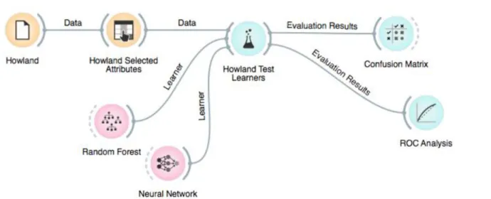
All data mining work was carried out using the Orange data mining toolbox for Python (Demsar et al. 2013). In addition to being compatible with Python for batch processing and the creation of custom tools, Orange offers a visual programming interface that can be downloaded at http://orange.biolab.si/. Initially, available data mining methods including naïve Bayes learner, k-nearest neighbors, neural network, classification tree, random forest, support vector machine, and CN2 rules methods, along with an ensemble method for combining multiple methods, were tested simultaneously to determine which produced the best classifications. Further information on algorithm implementation in Orange can be found at the Docs link on the above cited Orange webpage. A sample workflow is reproduced in Figure 3.
29
Figure 3: Sample Orange Workflow for Comparing Data Mining Methods
All the above listed data mining methods assess the performance of the classifications they produce by calculating the validity of the results the classification produces. Validity is assessed using several metrics to quantify potential sources of error. In addition to correctly classifying cases in a given category and rightfully excluding other cases from this category, it is also possible for error to be introduced in two ways: commission error (also referred to as Type I error or the false positive rate) quantifies the percentage of cases incorrectly classified in each possible category, while omission error (also known as Type II error or the false negative rate) quantifies the percentage of cases left out of the category in which they should have been included. In remote sensing datasets, known ground truth measurements are used to construct classification rules. These same cases are “blindly” classified according to these rules and the resulting differences are used to produce assessments of classifier performance and measures of classification accuracy. Overall accuracy or classification accuracy is determined by summing the number of correctly classified pixels (true positives and true negatives) and dividing by the total number of pixels to produce a ratio or percentage.
30
Similarly, classifications can be assessed for their accuracy for certain applications. User’s accuracy is calculated by dividing the number of correctly classified pixels in each category by the total number of pixels assigned to that category, and summing across all categories, thus summarizing the probability that the user of a classification will obtain a valid result. Producer’s accuracy compares the number of pixels correctly classified into each category to the original number of ground truth pixels used to characterize that category, thus summarizing the probability that the producer of a classification was able to train the classifier effectively for future applications. These metrics are calculated using a confusion matrix summarizing how each pixel was classified. These confusion matrices can also be used to calculate a summary statistic known as Cohen’s Kappa coefficient (Cohen 1960), which represents the degree of overall agreement between ground truth pixels and the classification being summarized. This metric is preferred to overall accuracy when comparing among studies or classification methods because it takes into account both user’s and producer’s accuracy (Congalton and Green 2009).
In addition to assessing the performance of a single classification method for any given dataset, different data mining methods used on the same dataset may be compared using several available indicators of performance. In this case, two such indicators were used: the area under the curve of the receiver operating characteristics graph (AUC-ROC) and the Brier Score. These methods of assessment rely on error metrics that are the related to the Type I and Type II error metrics discussed above; sensitivity (or the true positive rate) is the inverse of Type I error and specificity (or the true negative rate) is the inverse of Type II error. An ROC graph plots the rates of true positives against false positives, which is to say specificity versus the rate of Type I error. This comparison creates a curved hull, the area underneath which can be calculated and
31
compared across different classifiers. Since the area under the curve represents the probability that a random case will be classified as true positive rather than a false positive, a larger AUC-ROC score indicates better performance (Fawcett 2005). Brier curves accomplish a similar goal to ROC graphs, except that the curve it displays represents a metric of the cost of an incorrect classification across different operating parameters. As in an ROC graph, the area under this curve can be calculated, and is referred to as the Brier score (Hernandez-Orallo 2011). These two metrics are automatically calculated by Orange when comparing different data mining methods.
Three methods of resampling are also built in to the Orange visual programming interface. Resampling is a method of validation for data mining methods and can be carried out in several ways. Cross-validation resampling is performed by splitting the dataset into groups or “folds,” one of which is held out and compared to a classifier induced from the rest of the cases. This process is typically repeated several times. Leave-one-out resampling uses a similar technique, but holds out one case at a time instead of one group. Random sampling divides the dataset into two groups, for example by holding out 30% of cases as training data to be used for testing the remaining 70% of the cases. As with cross-validation resampling, this process is usually repeated several times, with a different random sample being held out in each repeat (Demsar et al. 2013). Each of these methods requires different computational time to accomplish, with the leave-one-out method being the most time-consuming.
2f. Refining LiDAR Metrics and Hyperspectral Data for Further Work
All previously discussed data mining method assessments were carried out on the outputs of classifiers run on the full lists of 32 LiDAR metrics, 43 vegetative indices, and 114 reflectance bands. However, one main goal of this study was to refine this list into a subset with high explanatory power. This was made possible using the Classification Tree Viewer widget in
32
Orange. This widget shows a list of details of each node in the classification tree created on a dataset. Since these nodes are chosen to break a dataset into smaller categories, they were assumed to be explanatory of the variability in the dataset as a whole. This method has previously produced promising results on a full-wavelength LiDAR dataset being used for tree species classification (Heinzel and Koch 2011). A similar method for variable reduction using the results of random forest-generated trees produced good results in a study using LiDAR data for forest inventory (Vauhkonen et al. 2010).
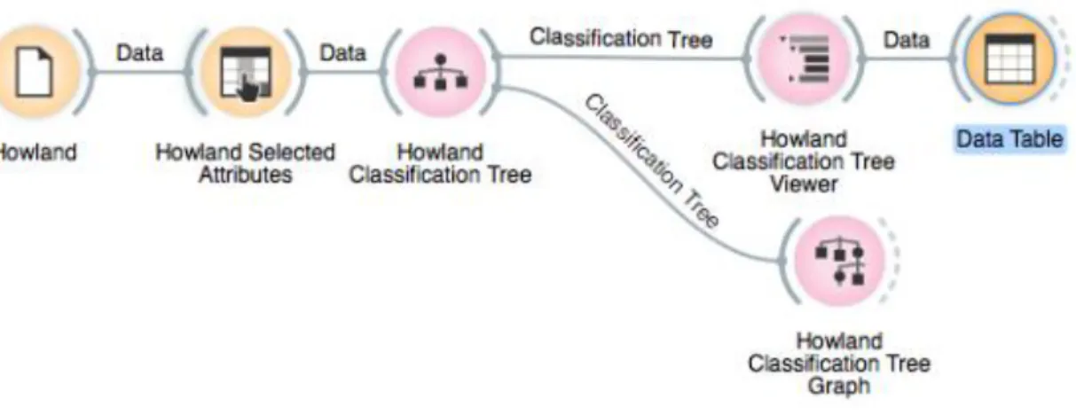
To apply this method here, a classification tree was run on each dataset, and the resulting list of variables used as nodes in the first five levels of each tree was kept for further work. This was done for the LiDAR metrics at each forest site and individually for the vegetative indices and for the reflectance bands at the Howland site. For the Howland site, another simplified list was produced from a combined input of all LiDAR and hyperspectral data. A sample workflow of the classification tree step can be found in Figure 4.
Figure 4: Sample Classification Tree Workflow
The results of the initial test of all data mining classifiers and resampling methods were used to determine the best settings for each dataset. These simplified and optimized settings and the refined list of metrics, indices, or bands were used to rerun the data mining procedure. A
33
sample simplified workflow can be found in Figure 5. In the case of the LiDAR metrics, a shared, or generic, set of metrics repeated across the simplified lists from the two forest sites, was generated and used as input for another set of classifiers. Classifier performance was again assessed by comparing AUC-ROC, Brier scores and classification accuracy generated by Orange. In all cases, the resampling method that produced the best results in the initial comparison was used for this assessment.
Orange does not provide built-in functionality for calculating the Kappa coefficient, so the confusion matrices generated by the Confusion Matrix widget were used as inputs for a custom Python script designed to calculate Kappa (see Appendix 1) for further classifier comparison. This script was designed to take advantage of the specific functionality of NumPy arrays (see van der Walt et al. 2013). This functionality allows for calculations to be performed simultaneously on the whole array or on a particular slice thereof, which is particularly useful for the conversion of data from confusion matrix to intermediate values used to calculate Cohen’s Kappa.
34
As a baseline for comparison, principal components analyses were also performed on the vegetative indices and reflectance hyperspectral files, using the Forward PC Rotation function in ENVI Classic. The resulting principal components with eigenvalues greater than one (nine total for the vegetative indices file and ten total for the reflectance file) were exported as geotiffs, processed in the same way as the original hyperspectral data, and used as inputs for data mining in Orange.
3. Results
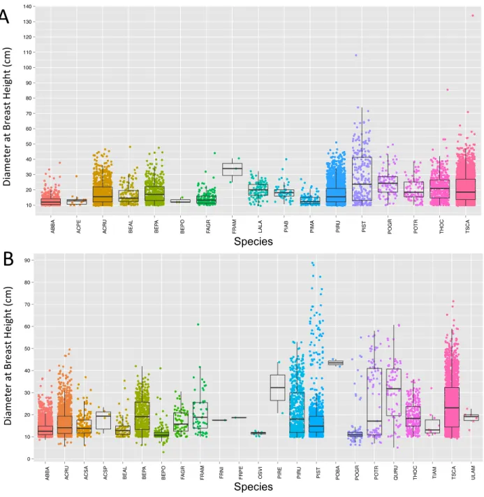
In order to confirm a relationship between structural variables and tree species, the diameter at breast height (DBH) data collected in the field campaign were plotted for each species class. Though individual tree heights were also recorded in some cases, there were too many missing values in the Penobscot dataset for a robust analysis or comparison. The trends in DBH by species can be seen as scatterplots in Figure 6 or as boxplots in Figure 7. While some patterns can be detected between overall tree size and species classification, DBH values alone do not seem to provide sufficient data to classify tree species on their own. An unexpected frequency of 10 cm as the recorded value for DBH also suggests that this value may have been used as a default measurement for small trees, and may be skewing distributions toward lower values overall. Additionally, DBH measurements are necessarily associated with the age of individual trees as well as their species. Nonetheless, the weak trends that can be detected suggest that further examining structural information on trees in the form of the LiDAR metrics is a sound avenue of analysis.
35
Figure 6: Plots of Individual Tree Diameter at Breast Heights by Species
Figure shows all available data points on diameter at breast height of individual trees in Howland Experimental Forest (A) and Penobscot Experimental Forest (B).
Initial comparisons of data mining methods and resampling techniques performed on all LiDAR metrics across Howland Experimental Forest and Penobscot Experimental Forest showed relatively consistent classification accuracy (CA) values across all combinations tested (Figure 7). While the data mining methods that produced the best results varied across the two forests,
36
leave-one-out resampling consistently allowed for the highest CA values. Using the LiDAR metrics alone, the highest classification accuracies achieved were CA = 0.5200 for Howland Experimental Forest, using a random forest classifier, and CA = 0.5215 for Penobscot Experimental Forest, using a neural network classifier. Second-best methods to be included for comparison on subsequent analyses included the classification tree method for Howland and the CN2 Rules method for Penobscot.
Initial comparisons of data mining methods and resampling techniques performed on vegetative indices for Howland Experimental Forest produced higher classification accuracy values than the same protocol run on LiDAR metrics (Figure 7). In this case, cross-validation resampling produced the highest CA values. Using the vegetative indices alone, the highest classification accuracy was CA = 0.6367, achieved using a neural network classifier. The k-nearest neighbors method produced a comparable classification accuracy of 0.6238, and was also kept for inclusion in subsequent analyses.
Initial comparisons of data mining methods and resampling techniques performed on reflectance data for Howland Experimental Forest produced classification accuracy values slightly lower than those from the vegetative index comparison (Figure 7). Cross-validation resampling again produced the highest CA values in this comparison. Using only data on the hyperspectral reflectance bands, the highest classification accuracy was CA = 0.6100, again achieved using a neural network classifier. The k-nearest neighbors and random forest methods produced comparable classification accuracies of 0.4981 and 0.5057, respectively. All three of these methods were kept for inclusion in subsequent analyses.
37
Figure 7: Comparison of Resampling Techniques and Data Mining Methods Using Complete Lists of Metrics
Available LiDAR data were used in separate analyses of each forest. Hyperspectral data (reflectance bands and vegetative indices) were only available for Howland Experimental Forest, so those analyses, as well as an analysis of all available data together, were only conducted for that site. Repeated colors in the same column indicate the results of different resampling methods used in combination with each classifier.
Another initial comparison of data mining methods and resampling techniques was performed, this time on all available data for Howland Experimental Forest (Figure 7). Cross-validation resampling once again produced the highest CA values in this comparison, CA =
0.52
0.5215
0.6367
0.61
0.6371
0.5199 0.5029 0.5108 0.6238 0.6326 0.4981 0.4681 0.5944 0.6019 0.6224 0.05 0.10 0.15 0.20 0.25 0.30 0.35 0.40 0.45 0.50 0.55 0.60 0.65 Howland LiDAR + Hyperspectral LiDAR Howland LiDAR Penobscot Reflectance Vegetative Indices C la s s if ic a ti o n A c c u ra c y Classifier Classification Tree CN2 Rules k−Nearest Neighbors Naive Bayes Neural Network Random Forest38
0.6371, achieved using a k-nearest neighbors classifier. The neural network method produced a comparable classification accuracy of 0.6019, and was also included in further analyses.
As described above, classification trees were also run on each dataset discussed above, regardless of the performance of this method during the initial comparison. These classification trees were not used to generate metrics of classifier performance, but were viewed in list format in order to identify which metrics, indices, or bands served as the nodes in the first five levels of the tree. The results of that analysis provided simplified lists of inputs for use in further analyses (Table 5). A list of thirteen LiDAR metrics from Penobscot Experimental Forest and a list of ten LiDAR metrics from Howland Experimental Forest were cross-referenced to produce a generic list of five LiDAR metrics shared between the classification trees produced on the two forests. This generic list was generated in an attempt to identify some universal or generalizable aspects of LiDAR data that may have strong explanatory power in other forests. The hyperspectral data available on the Howland site were also used to produce simplified lists of reflectance bands, vegetative indices, and a list generated from the full dataset of LiDAR and hyperspectral data together. All further results were generated using only the inputs shown in these simplified lists.
39 Table 5: Simplified Lists of Data Mining Inputs
Penobscot Howland Generic LiDAR LiDAR Metrics LiDAR Metrics Reflectance Bands Vegetative Indices Hyperspectral + LiDAR D9 Fcover Fract_all P50 P100 D0 D2 D9 Fcover Fract_all Kurtosis Mean P10 P40 P50 P80 P100 St_Dev D3 D5 D6 D9 Fcover Fract_all P50 P60 P90 P100 B003 B019 B026 B037 B038 B054 B059 B062 B063 B070 B072 B079 B086 B102 B112 B113 ARI1 ARI2 CRI2 DATT2 GI GM2 PRI RDVI RGRI SIPI B023 B034 DATT2 Fract_All GM1 GM2 Mean MTCI P60 P70 PRI REIP RGRI SIPI VOG
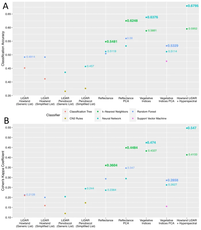
The classifiers that produced the best results using the LiDAR metrics from both forests as inputs were run again, using only the simplified and generic lists discussed above. At this stage, final comparisons were made by adding in the Cohen’s Kappa coefficient as an additional means of assessing the performance of these optimized protocols. Figure 8 shows the results of classifications run on the simplified and generic LiDAR metrics datasets, using the two best data mining methods for each forest as determined by the initial comparison of classifiers.