Exploiting multiple levels of parallelism of Convergent Cross Mapping

(1)

Exploiting multiple levels of parallelism of

Convergent Cross Mapping

A Thesis Submitted to the

College of Graduate and Postdoctoral Studies

in Partial Fulfillment of the Requirements

for the degree of Master of Science

in the Department of Computer Science

University of Saskatchewan

Saskatoon

By

Bo Pu

c

(2)

Permission to Use

In presenting this thesis in partial fulfilment of the requirements for a Postgraduate degree from the University of Saskatchewan, I agree that the Libraries of this University may make it freely available for inspection. I further agree that permission for copying of this thesis in any manner, in whole or in part, for scholarly purposes may be granted by the professor or professors who supervised my thesis work or, in their absence, by the Head of the Department or the Dean of the College in which my thesis work was done. It is understood that any copying or publication or use of this thesis or parts thereof for financial gain shall not be allowed without my written permission. It is also understood that due recognition shall be given to me and to the University of Saskatchewan in any scholarly use which may be made of any material in my thesis. Requests for permission to copy or to make other use of material in this thesis in whole or part should be addressed to:

Head of the Department of Computer Science 176 Thorvaldson Building 110 Science Place University of Saskatchewan Saskatoon, Saskatchewan Canada S7N 5C9 Or Dean

College of Graduate and Postdoctoral Studies University of Saskatchewan 116 Thorvaldson Building 110 Science Place Saskatoon, Saskatchewan Canada S7N 5C9

(3)

Abstract

Identifying causal relationships between variables remains an essential problem across various scientific fields. Such identification is particularly important but challenging in complex systems, such as those involv-ing human behaviour, sociotechnical contexts, and natural ecosystems. By exploitinvolv-ing state space reconstruc-tion via lagged embeddings of time series, convergent cross mapping (CCM) serves as an important method for addressing this problem. While powerful, CCM is computationally costly; moreover, CCM results are highly sensitive to several parameter values. Current best practice involves performing a systematic search on a range of parameters, but results in high computational burden, which mainly raises barriers to practical use. In light of both such challenges and the growing size of commonly encountered datasets from complex systems, inferring the causality with confidence using CCM in a reasonable time becomes a biggest challenge. In this thesis, I investigate the performance associated with a variety of parallel techniques (CUDA, Thrust, OpenMP, MPI and Spark, etc.,) to accelerate convergent cross mapping. The performance of each method was collected and compared across multiple experiments to further evaluate potential bottlenecks. Moreover, the work deployed and tested combinations of these techniques to more thoroughly exploit available computation resources. The results obtained from these experiments indicate that GPUs can only accelerate the CCM algorithm under certain circumstances and requirements. Otherwise, the overhead of data transfer and communication can become the limiting bottleneck. On the other hand, in cluster computing, the MPI/OpenMP framework outperforms the Spark framework by more than one order of magnitude in terms of processing speed and provides more consistent performance for distributed computing. This also reflects the large size of the output from the CCM algorithm. However, Spark shows better cluster infrastructure management, ease of software engineering, and more ready handling of other aspects, such as node failure and data replication. Furthermore, combinations of GPU and cluster frameworks are deployed and compared in GPU/CPU clusters. An apparent speedup can be achieved in the Spark framework, while extra time cost is incurred in the MPI/OpenMP framework. The underlying reason reflects the fact that the code complexity imposed by GPU utilization cannot be readily offset in the MPI/OpenMP framework. Overall, the experimental results on parallelized solutions have demonstrated a capacity for over an order of magnitude performance improvement when compared with the widely used current library rEDM. Such economies in computation time can speed learning and robust identification of causal drivers in complex systems.

I conclude that these parallel techniques can achieve significant improvements. However, the performance gain varies among different techniques or frameworks. Although the use of GPUs can accelerate the appli-cation, there still exists constraints required to be taken into consideration, especially with regards to the input data scale. Without proper usage, GPUs use can even slow down the whole execution time. Convergent cross mapping can achieve a maximum speedup by adopting the MPI/OpenMP framework, as it is suitable to computation-intensive algorithms. By contrast, the Spark framework with integrated GPU accelerators still offers low execution cost comparing to the pure Spark version, which mainly fits in data-intensive problems.

(4)

Acknowledgements

To begin with, I would like to express my genuine gratitude to my supervisor, professor Nathaniel D. Osgood, for the continuous support of everything during my master study here with his patience, motivation, and immense experience. I could not have imagined having a better advisor. During my study period here, I have learned a lot from my supervisor not only on the academic level but also in his high ethical standards. His enthusiasm, generosity, care for others and passion for research are influenced me deeply, which will always remind me to become a better person in my rest life. Moreover, I take it as one of the luckiest things in my life to study and work with my supervisor. Besides my advisor, I would like to thank the rest of my thesis committee: Prof. Dwight Makaroff, Prof. Derek Eager, and Prof. Francis Bui, for their insightful comments and thoughtful suggestions. And also for the questions which incented me to widen my research from various perspectives.

Also, I would like to acknowledge my fellow lab mates in for the stimulating discussions, for the sleepless nights we were working together before deadlines, and for all the fun we have had in the last two years. Mainly, I would like to thank Weicheng Qian, Yang Qin and Lujie Duan for the advices on parallel implementations; Weicheng Qian offers tremendous help and support in the implementation details and theory discussion based on his knowledge. Lujie Duan provides a lot of insights when we discuss the cluster configuration and system-level problems. I would also like to thank all the professors and stuff in the computer science department, especially Christine, Sophie and Gwen for their guidance during my master study period.

Finally, I want to thank my family for the support when I study here. I haven’t have the chance to go back China when I came here two years ago. My mother Dirong Chen and my father Shaoming Pu take care of everything so I can pursure my master degree without any concern. Your love, support and encouragement are always my impetus to move forward.

(5)

List of Tables

2.1 Notation . . . 17 4.1 Baseline setting . . . 40 4.2 Implementation Levels . . . 41 4.3 Elasticity Analysis . . . 42 4.4 Cluster Configurations . . . 45

5.1 Hardware configuration of the hybrid cluster . . . 56

5.2 CCM baseline parameters setting . . . 57

(8)

List of Figures

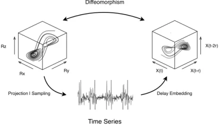
1.1 This diagram demonstrates the methodology of attractor reconstruction via delay embedding. The true attractor is projected into a time series by some measurement functions, from which an image of the attractor can be formed by delay reconstruction, up to some diffeomorphism. 3 2.1 GPU device architecture overview. . . 14 2.2 Shared memory system architecture overview. . . 14 2.3 Distributed memory system architecture overview. . . 15 3.1 Image adapted from [53] illustrates the kNN search problem given the embedding dimension

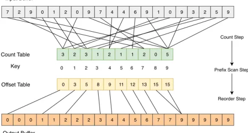
parameterE= 3, which means thatk is 4, in the reconstructed state space. The blue points refer to the points inRP set while the red points are inQP set. Reflecting the fact thatk= 4, the circle gives the distance between the query point and the fourth closest reference point. . 22 3.2 An example of a pass in the radix sorting operation on one chunk of length n = 20 within

4-bit digits, which means that the maximum value is less than 24_{= 16. . . .} ₂₄

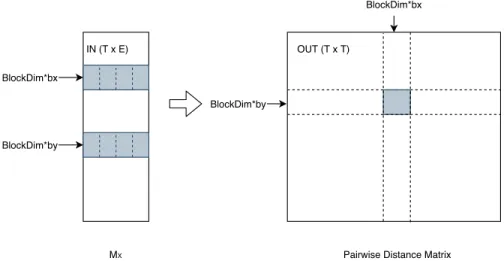
3.3 An illustration of applying the radix sort to sortk= 8-bit integers by 2 passes of three steps aforementioned ond= 4-bit integers from the least significant bits to the next higher significant bits, and so on. . . 24 3.4 The parallel algorithm for pairwise distance calculation. Each block computes one sub-matrix

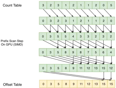
of OUT, and the threads work on one pair of aligned sub-matrices of IN, as is illustrated as the figure. . . 26 3.5 The parallel prefix scan algorithm. The interval is changed from 1 to intervallog2n. . . 27

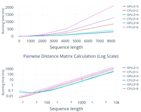
3.6 The parallel algorithm for R samples, (E + 1)-dimension vectors, of Pearson’s correlation coefficient calculation. Each thread computes one row of OUT, which takes one pair of the same row of XandY. . . 28 3.7 The performance comparison of the pairwise Euclidean distances under different dimensionE

and the input sequence lengthT (Notably, then input matrix isT×E). . . 29 3.8 The performance comparison of the radix sort operation in kNN search when applying the

distances calculated from previous step. Sort can be performed either on local library sizeL

or global time seriesT. . . 30 3.9 The performance comparison of Pearson’s correlation coefficient computation for twoR×[E+1]

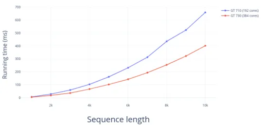
matrices given a certain library sizeL. . . 31 3.10 Among three kernel functions, the pairwise distance calculation kernel takes much longer time,

which can be utilized as the benchmark to compare the performance of different GPUs. . . . 32

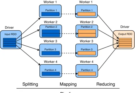
4.1 Simplified typical hybrid MPI/OpenMP scheme applied on CCM. . . 35 4.2 An example of the pipeline running distributed on Spark. . . 37 4.3 A diagram of CCM RDD transformation which takes multiple realizations as input and outputs

prediction skills. . . 37 4.4 An illustration of the dependencies of two pipelines. After the distance indexing table is

constructed in parallel, Spark will broadcast it to all nodes. In the next pipeline, the executors can look up in the table and fetch theE+ 1 nearest neighbours quickly. . . 38 4.5 A diagram of Spark executing asynchronous pipelines. . . 39 4.6 The 3-node cluster contains 3 machines, which has been labelled from 0 to 2. Node 0 is the

master node in the cluster and the machine which runs rEDM for comparison. . . 40 4.7 Yarn Mode utilizes all worker nodes in the cluster, while Local Mode only runs experiments

on the master node. Yarn Mode significantly diminishes the average computation time of the parallel version of CCM with the help of worker nodes. . . 42 4.8 The parallel version uses all of the optimization methods with five 4-core workers in the cluster,

while the single-threaded version is only executed on the master node without any parallel optimization. . . 43

(9)

4.9 The single-threaded version without using Spark consumes little time to finish when library sizeLis small. However, with increasingL, the time to search for nearest neighbors in a larger shadow manifold and the time to complete grows superlinearly. . . 44 4.10 The average running time can be reduced when more computational resources are available

in the cluster. Under the same total computational resources, the computation time is larger with more inferior worker nodes given the rising time cost of networking I/O. . . 45 5.1 An overview of the GPU-enabled cluster. . . 49 5.2 A comparison of pure Apache Spark and Apache Spark with external program implementation. 50 5.3 CPU utilization plot in the cluster for three workers. . . 52 5.4 Overall methodology of integrating GPU with Spark framework. . . 52 5.5 Bottleneck elimination and performance comparison after introducing GPU into external

ap-plication. . . 53 5.6 The comparison between pure MPI with CUDA and CUDA-Aware MPI architecture.

Ob-viously, CUDA-Aware MPI provides a layer to unify the memory space between host and device. . . 54 5.7 Simplified hybrid CUDA-Aware MPI/OpenMP scheme applied on CCM. . . 55 5.8 This experiment is conducted in the cluster setup described in the Table 4.1. The computation

part and disk I/O part are separately measured to compare with respect to differences in each. 58 6.1 The best speedup of Parallel CCM achieved in this thesis, when compared to rEDM. . . 62

(10)

List of Abbreviations

CCM Convergent cross mapping

RDD Resilient distributed datasets in Spark MPI Message passing interface

GPU Graphics processing units FPGA Field-programmable gate array kNN k nearest neighbors framework

MIC Intel Many Integrated Core that combines many cores onto a single chip UVA Unified Virtual Addressing in CUDA-aware MPI

(11)

Chapter 1 Introduction

1.1 Motivation

1.1.1 Detecting Causality using Convergent Cross Mapping

The detection of causality in complex systems has been studied for many years, in light of its importance for scientific study, design of models, decision-making, and other needs. Complex systems are referred to the systems whose behaviour is difficult to understand due to the fact that system behaviour is not directly understandable through understanding each component of the system in isolation. For such systems – where the “whole is greater than the sum of the parts”, behaviour exhibits non-linear relationships on system states and depends heavily on hidden dependencies or unknown interactions caused by the inside (parts of the systems) or outside factors (environment) of the systems. However, systems involving various interacting variables and potential states are fundamental to the natural and social sciences.

The authentic causal understanding of such systems through their behaviours plays an essential role given the need to making effective decisions, especially including policy and financial domains [58]. In traditional analysis – inspired by linear systems – identification of correlation and covariation between variables has been widely applied in hopes of identifying causality in stationary time series. By contrast, complex non-linear system variables can be positively linked at specific time windows, while at other time windows, such variables can appear unrelated or even negatively linked. Such conflicting evidence will often arise when traditional metrics like correlation and covariation are applied. Analysis using correlation or covariation becomes more difficult to justify with increasing recognition that nonlinear dynamics are ubiquitous in chal-lenging decision-making and policy contexts. Although linear dynamic analysis is a well-developed technique with elegant theoretical underpinnings, most real-world systems manifest themselves in a much broader spec-trum of possible complex behaviours. Possibilities include intermittency, discontinuous motion, and history dependence, including sensitivity to initial states. All of these seeming chaotic behaviours make complex systems unpredictable and challenging to understand. Furthermore, the methods, which are designed based on the linear systems, can lead to incorrect or even contradictory evidence regarding causality in nonlinear systems. Increasing recognition of the importance of such behaviour calls for a better criterion to evaluate causal connections in complex systems.

(12)

Different approaches have been pursued to overcome the difficulty associated with causal inference in complex systems. Firstly, controlled experimentation or investigation of underlying mechanisms have been applied to investigate causal relations among variables. The first of these requires a substantial investment of time and financial resources. For contexts in which we seek to understand human behaviour, the pursuit of controlled experiments frequently poses ethical concerns, due to the risk of imposing harm on subjects. The limits of such controlled studies – such as Randomized Controlled Trials (RCTs) – are particularly notable in the context of complex systems, which commonly exhibit reciprocal feedbacks, delays and non-linearities [38].

While research seeking to elucidate underlying mechanisms and causal pathways (e.g., biological pathways underlying certain types of cancer, or diseases such as Type 2 Diabetes) are ubiquitous in science, the time required to secure great progress in such studies is commonly measured in decades.

The limitations of such traditional routes to identifying causal linkages have driven investigation into alternatives. [26] sought to take advantage of Granger causality (GC) theory as a mechanism for testing nonlinear causality in time series. But this approach can be problematic, especially in weak to moderate coupling systems [53]. The method exhibits particular limitation on account of its assumption of separa-bility. While separability [36] is characteristic of completely stochastic systems, in complex systems with the capability of displaying broad coupling, separability typically does not hold. Separability represents the perspective that the systems can be reconstructed piece-by-piece rather than as a whole, which flies in the face of the emergent behaviour routinely seen in complex systems. The assumptions of the GC method apply only under the condition that completely stochastic is the nature of the real world. However, most of the systems in the real world contain strong deterministic governing components, which behave with patterns. As such, dynamic systems theory can be fruitfully introduced to analyze principles underlying the dynamics of complex, non-linear systems, and to reason about their long-term qualitative behaviour.

1.1.2 Dynamical System Theory

Dynamical system theory [2] is a scientific area, generally employing mathematical methods such as differential or difference equations, to describe and understand the behaviour of complex systems. At any timepoint, a dynamical system has a state characterizable by a vector, which can be alternatively viewed as a point with finite dimensions in accompanying state space. In dynamic system theory, such states can evolve under certain deterministic or stochastic rules that provide guidelines as to how current state evolves into future state. Mathematical characterization of state and its time evolution (behaviour) form the foundation of this theory.

To the extent that the system is deterministic and dynamics are not entirely random, there will be an underlying manifold controlling the dynamics. As such, this theory introduces the concept of an attractor. Causally linked time-series variables share a common attractor manifoldM, which means that the coordinate for one state space coordinate will typically be closely covarying with another, and the information associated

(13)

with one variable can be recovered from variables that it drives within the dynamics of the common attractor. Hence, reconstruction of nonlinear state space M0 can serve as an important possible tool when seeking to infer causality in a dynamic system.

1.1.3 Takens’ Embedding Theorem

In 1981, Takens’ Theorem [55] demonstrated and proved the manner in which lagged coordinates formed by a time series could be employed as substitute variables to reconstruct the shadow manifold of the underlying dynamic system. AssumingM is a compressed manifold of am-dimension state space, so a dynamical system actually can be thought as a diffeomorphism φdetermining the trajectories on the compressed manifold M

under the discrete time intervals in Takens’ Theorem [13]. The reference to the diffeomorphism refers to the invertible function that maps two smooth manifolds whilst preserving similarity on local topology. In mathematics, givenφandM, an observation functiony:M −→Rcan be applied to construct an embedding M0ofM in 2m+1 dimensions. The complete transformation form in Takens’ Theorem is Φ(φ,y):M −→R2m+1,

where Φ(φ,y)(X) =< y(X), y(φ(X)), y(φ2(X)), ..., y(φ2m(X))>[13]. Here, the components on the right side

of the equation represent the time-lagged variables of the original dynamics onM. As we can observed from the equation, such mappings (in the observation function) involve a single time series, which only represents a subset of possible mappings when considering the number of time series and lagged values. The reconstructed embedding may not preserve the global topology information of original manifoldM. But still, the every local neighbourhood in the topology of the original manifold can be preserved, which remains a useful conceptual stepping stone for information recovery by searching nearest neighbours of reconstructed embedding manifold

M0.

Projection | Sampling Delay Embedding

Time Series Diffeomorphism X(t) X(t-r) X(t-2r) Rz Rx Ry

Figure 1.1: This diagram demonstrates the methodology of attractor reconstruction via delay em-bedding. The true attractor is projected into a time series by some measurement functions, from which an image of the attractor can be formed by delay reconstruction, up to some diffeomorphism.

As shown in Figure 1.1, the real attractorM, usually characterized as a surface or manifold, is defined by the trajectories in three-dimensional space. For simplicity, a manifold can be considered as a generalized,

(14)

E-dimensional surface embedded in some higher dimensional space, where the dimension of the manifold may be irregular and fractal. In equation (1.1), the time seriesX (whereT is maximum index) can be viewed as sequential projections of the motion or samples with a certain time interval on the real attractorM in the dynamic system, as follows.

X =< x1, x2, ..., xT > (1.1)

Takens’ Theorem above states that mathematically valid and equivalent reconstructions M0 of the at-tractor can be created using lags of just a single time series (a sequential projection) by substituting those lagged values for unknown or unobserved variables, as each time series is a function of the system state and in general is driven by – and thus contains information regarding – several state variables. In equation (1.2),

E= 2m+ 1 is the reconstruction embedding dimension andτ (τ >0) is the general delay as lagged value.

− →

xt=< xt, xt−τ, ..., xt−(E−1)τ> (1.2)

1.1.4 Convergent Cross Mapping

Convergent cross mapping [53], proposed by Dr. George Sugihara in 2012, is a statistical test based on Takens’ Theorem that can be used to detect and help quantify the relative strength of unidirectional and bidirectional causal relationships between two variables X and Y drawn from the same coupled complex system. Essentially, to investigate whether Y is causally influencingX, we determine whether the shadow manifold MX encodes information about Y. To do so, we take advantage of the fact that if Y is

govern-ing/driving/influencingX, the value of Y is part of the state of the system underlyingX. By the definition of state space, information concerning the state (and, thus, value) ofY would need to be captured (encoded) by the location in the state space of the system driving X. By contrast, if Y is not drivingX, Y does not form an element of the state space of X, and the location in state space of the system driving X should not encode any more information about the value of Y than mere statistical dependence on another aspect of state. Then we assess whether (and to what degree) it is possible to estimate (infer) the value ofY at a given time t using information from the observation ofY associated with the closest points within shadow manifold MX reconstructed from the delay embeddingX. If the ability to use X to recoverY rises as one

considers shadow manifolds of additional density – and reconstructed from longer time series – it suggests that Y is driving X. By contrast, a merely statistical dependence of Y on an element of the system state underlying X or X itself would not lead to a notable rise in the ability to predict Y with shadow manifold density.

More specifically, the algorithm uses lag embedding of time seriesX to reconstruct the shadow manifold

MX [31]. To rebuild a state space of dimensionalityE – including unobserved (latent) variables within the

system – from a time seriesX, we can substitute each (non-boundary censored) point of that time series by anE-dimensional vector whose elements are successive lagged values drawn from that time series separated

(15)

by time index τ, per equation (1.2). Within the CCM algorithm, in order to assess if variableX is causally governed by variable Y, we attempt to predict the value ofY on the basis of the state space reconstructed from X (see below); for statistical reliability, this must be performed over a large number Rof realizations. To assess causality, we examine whether these results converge as we consider a growing number Lof data points – and thus a greater manifold density – withinX within our reconstruction (see below).

Overall, the results of CCM are sensitive to the parameters below (the overall notation of CCM is listed in Appendix A):

E: This parameter is the estimated embedding dimension of the dynamic system. For simplex projection,E

will typically range from 1 to 10. Eckmann [16] demonstrated the fundamental limitations for estimating dimensions of dynamic systems in 1992. The difficulty of accurately estimatingE requires researchers testing and running CCM for different possible values ofE.

τ: This fundamental parameter represents the embedding delay used in shadow manifold reconstruction. If appropriate lags are used, the reconstruction preserves the essential mathematical properties of the original system: Reconstructed states will map one-to-one to actual system states, and nearby points in the reconstruction will correspond to similar system states. In the presence of high autocorrelation between successive measured values in X, smaller values of τ will lead to successive coordinates in the embedding vector holding highly similar values; by contrast, larger values of this parameter will yield embedding vector elements less subject to autocorrelation. However, the estimation of the most favorable embedding delay is often unclear, and current practice explores a variety of possible values.

L: Another parameter central to the definition of CCM,Lcounts the size of the subsequence of the embed-ded library extracted from the time series for the purposes of state space reconstruction. In general, a prediction skill that initially increases along with risingLand then converges with a positive plateau value implies a causal relationship. With more data, the trajectories defining the attractor fill in, result-ing in closer nearest neighbours and declinresult-ing estimation error (correspondresult-ing to a higher correlation coefficient) asLincreases.

R: This parameter – whose notation is less standardized in the literature – refers to the count of random subsamples (realizations) taken of a given size L. To enhance statistical reliability, the value ofR is commonly set to 250 or larger. By determining the statistical confidence associated with the tests, this parameter is an important feature of any empirical study and statistical measurement. In the algorithm, multiple random realizations for a given library sizeLcan reduce bias, produce more accurate estimates, and better reveal trends with growingL. Alternatively with researchers using larger sample sizes, higher values of this parameter impose elevated levels of computational burden in the form of longer running times and elevated space consumption for CCM output.

Running CCM across a wide range of different parameter settings is necessary to obtain a reliable causal reference (hyperparameter tuning), and thus imposes a relatively high computational overhead. As for

(16)

various data science tasks, parallel and distributed processing can enhance the computational performance and shorten the execution latency.

In this thesis, following additional background on CCM and the literature of parallel techniques, we de-scribe different versions of CCM parallel implementation which take advantages of contemporary parallel and distributed processing techniques. For instance, the CUDA framework [37] provided by NVIDIA GPUs, the MapReduce framework [12] provided by Apache Spark (henceforth, “Spark”) and the hybrid [50] framework provided by MPI/OpenMP will be studied and applied on CCM. The thesis then presents an informal perfor-mance evaluation and comparison of these frameworks. We conclude from the experiments that, with parallel techniques and cloud computing support, researchers can use CCM to confidently infer causal connections between larger time series in far less time than is required by extant libraries implementing the general CCM algorithm.

1.2 Research Goals

As mentioned earlier, Convergent Cross Mapping is an algorithmic technique based around the idea of shadow manifolds reconstructed via lag coordinate embedding. In order to estimate the causal relationship with confidence, proper parameters E, τ for the dynamic systems should be applied. Another limitation of CCM concerns the library size Land sample size R. Inference of the causal relationship is based on how ρ

changes along withL, as judged by a sample ofRsuch values for each value ofL. Determining the ensemble of such values ofρimposes a heavy computation workload. CCM has been restricted in its range of application because of the high computational complexity; for example, while the length of modern time series may run into the millions, use of rEDM with values ofLin the range of just 5000 can require overnight computation. To address the computational disadvantages of CCM, variants for the algorithm have been considered and offer significant results. However, these studies suffer from other limitations, and they do not offer a general solution.

This thesis seeks to investigate means of supporting scientifically reliable causal inference and prediction in a reasonable time by applying multiple levels of parallelism on convergent cross mapping. In consideration of the increasing availability of affordable computer hardware supporting parallel computation in recent years, various algorithms have been redesigned to take full advantage of computational resources. For example, the application of deep learning has been made more accessible on account of the fact that the matrix-based networks can be accelerated using GPUs. Additional Big Data related topics have become popular following the decreasing cost of computer hardware, and the introduction of cluster computing. The thesis being investigated here is that, subject to availability of sufficient computational resources, the parallel implementation of CCM will dramatically reduce the computation time required to conduct the analyses of causality.

(17)

1.3 Thesis Organization

The thesis is organized as follows. Chapter 2 provides background regarding both convergent cross mapping and several parallel processing techniques. This chapter includes a literature review on the foundational papers characterizing the CCM technique, as well as current work which improves the performance of CCM in certain conditions, and its related applications. Chapter 3 introduces possible methods for GPU acceleration and optimization when performing CCM on a single machine. The performance comparison between CPU and GPU will be presented. The concluding section of the chapter will summarize the advantages and limitations of GPU acceleration. Chapter 4 follows the emphasis on parallel implementation by extending the parallel techniques to take advantage of clusters of machines in which implementations based on MPI and Apache Spark will be discussed and compared. Chapter 5 combines the parallel techniques proposed in Chapter 3 and chapter 4 to more fully exploit multiple levels of parallelism. However, the use of multiple parallel technologies elevates code complexity and imposes performance bottlenecks. Also, this chapter lays out an evaluation and discusses possible solutions. Finally, chapter 6 provides a concluding summary of this research and discusses the contributions of this thesis as well as promising prospects for future work.

(18)

Chapter 2 Background

2.1 Literature Review

There are two subareas of the literature relevant to the research purpose of this thesis: Convergent Cross Mapping and parallel and distributed programming techniques. Convergent Cross Mapping basics covered here focus on the essentials of the theory and recent applications. Past work on CCM improvements will be listed and compared based on their advantages and disadvantages. The coverage of background on parallel techniques introduces the reader to a subset of prominent existing parallel models and frameworks affording ready application to convergent cross mapping to improve the computation speed. Parallel methods covered relate to two primary types of resources: The hardware architecture (which we call parallel computers) and its corresponding parallel software models. The resulting parallelization is achieved with the support of both hardware and software implementation.

2.1.1 Convergent Cross Mapping Basics

In 2012, Sugihara [53] built on ideas from Takens’ Theorem [55] to propose convergent cross mapping (CCM) to test causal linkages between non-linear time series observations. This approach has enjoyed diverse appli-cations. For example, Luo [39] successfully revealed underlying causal structure in social media and Verma [57] studied cardiovascular and postural systems by taking advantages of this algorithm.

In empirical dynamic modeling, time series – samples on the time axis – reflect the system states or behaviors, and can be understood as sequential projections of the underlying state of the associated complex system. In accordance with the theory of time series embedding, such a time series encodes information about the aspects of the system state that govern this variable. By Takens’ theorem, to reconstruct a state space of dimensionalityE – including unobserved (latent) variables within the system –, we can substitute each point of that time series by an E-dimensional vector whose elements are τ lagged values drawn from that time series. In order to assess if variable X is causally governed by variableY in CCM, we attempt to predict the value of Y on the basis of the state space reconstructed fromX (see below). For statistical reliability, this prediction must be repeated over a large number R of realizations. To assess causality, we examine whether these results “converge” as we consider a growing numberLof data points withinX within our reconstruction (also see below).

(19)

We provide here a brief intuition for why and how CCM works. Consider two variables X andY, each associated with eponymous time-series and – further – whereX depends onY. For example, consider a case where for each time pointX measures the count of hares, andY that of lynx. IfX (hares) causally depends on Y (lynx), the dynamics of X (e.g., a rapid rise or persistent drop in the hare population) will often tell us much about the state of other areas of the system that governs it, includingY (e.g., that there are likely to be few or many lynx around, respectively). The converse is true as well, if Y (lynx) causally depends on

X (hares), observing the values of Y over time (e.g., a steep drop or a plateauing in lynx numbers) tells us about the state of governing factors, includingX (here, the fact that the number of hares is too small to feed the lynx population effectively, or that they are roughly in balance with lynx, respectively). An implication of the first of these cases, whereX depends onY – captured by Takens’ Theorem – is that information on the state ofY is encoded in the state space reconstructed fromX, meaning that points that are located nearby withinX’s reconstructed state space will be associated with similar values forY, and can thus be used to make accurate (skillful) prediction of the value ofY. In most cases, such prediction of one variable (e.g.,Y) within the reconstructed state space of another (X) can be achieved by nearest neighbor forecasting using simplex projection [54] – that is, by considering the contemporaneous value ofY associated with the nearest neighbours to the point being considered in shadow manifoldMX. Pearson’s correlation coefficient between

observed and predicted values ofY can be applied over a “library” of a given lengthLto measure prediction skill. Details regarding the CCM algorithm can be found in Section 2.3.

Simplex Projection

Simplex projection, employed by convergent cross mapping, can be a valuable tool to distinguish chaotic time series from random noise. The central idea behind this tool is that the behavior of similar events in the past can directly forecast the events in the future. For the sake of simplicity, it involves tracking the evolving forward pattern among nearby points in the embedding manifold we reconstruct using lagged values. So, it belongs to a kind of nearest-neighbor forecasting algorithm with relatively high computational complexity.

There are two parameters associated with the simplex projection stage of CCM: Embedding dimension

E and lag τ to create lagged-coordinate vectors for the manifold MX. A high-fidelity one-to-one map will

be presented between the reconstructed attractor and original attractor if the appropriate parameters are chosen. If the estimation of E is smaller than the appropriate one, the reconstructed states will directly overlap with each other, as they exhibit separation and structure higher dimension that may project to the same region of lower embedding dimension. As such, poor estimation of the parameter E can lead to poor forecast performance, and, as a result, the system behaviors cannot be captured within the reconstructed shadow manifold. Sugihara & May [54] use prediction skill as an indicator to identify whether E is the optimal embedding dimension. In this paper, the author argues that if we observe that forecast skill peaks at E = 2, it indicates that the real attractor manifold underlying input time series are unfolded best in 2 dimensions, which means E should be 2 to best approximate the real embedding dimension. Another

(20)

similar concept relates the actual dimensionality of the dynamic systems, which is not an exact equivalent to the embedding dimension. Estimation of the actual dimension of the corresponding dynamic systems should consider additional factors, including observational error, process noise, and time series length, and the system modes. Notably, the actual dimensionality of a dynamic system is often determined by the underlying state variables associated with it, while the dimensionality of the manifold E is the dimension that gives the highest prediction skill, which generally smaller than the actual dimensionality of the state space in complex systems [39].

Pearson’s Correlation Coefficient

When applied to a sample, Pearson’s correlation coefficient – also called the sample Pearson correlation coefficient, or simply put as the sample correlation coefficient – is commonly represented byrxyorρxy. This

metric is widely used across various domains to measure the relation between observations. In CCM, the (Pearson) correlation coefficient between a sample predicted and a sample of observed values is treated as the prediction accuracy (skillfulness), which primarily serves as testing the degree to which information regarding

Y is captured within the state space ofX. Closely resemblant local topological structures suggest a causal connection between time series Y and X. With the correlation coefficient, evaluating such prediction skill becomes less computationally intensive and is relatively straightforward. Given two sequences in any of the sample, predicted valuespyand corresponding valuesyof equal lengthE+ 1 (representing theE+ 1 nearest neighbors found in BF kNN search), the Pearson’s correlation coefficient between two sequences is defined as the covariance of the two sequences divided by the product of their standard deviations. That is, given paired data{(py1, y1), . . . ,(pyE+1, yE+1)} consisting of (E+ 1) pairs,rpy,y is defined as:

rpy,y= PE+1 i=1 (pyi−py)(yi−y) q PE+1 i=1 (pyi−py)2 q PE+1 i=1 (yi−y)2 (2.1)

Where py and y are the sequence mean for py and y, respectively. However, the standard correlation coefficient is just one of several alternative measures of the agreement between predicted and observed values. There are some other methods that have been applied to measure the prediction accuracy. Mean absolute error of predictions (MAE) and root mean squared error of predictions (RMSE) serve as alternative measures to the Pearson correlation coefficient metric when measuring skillfullness. The reporting of skillfulness using such metrics can be supported by the Sugihara research group’s contributed public library rEDM. However, among these metrics, the Pearson’s correlation coefficient remains the most commonly used, and the parallel implementations in this thesis only consider this measurement in producing reliable prediction results across an ensemble of Rdifferent samples.

(21)

Identify Causality

A key need within CCM is to distinguishcausal dependence of one variable on another from purely statistical dependence (e.g., due to covariation) – which might also support high prediction skill within a given recon-structed manifold. The two can be distinguished by assessing how prediction skill changes as the number data points used in the embedding – the so-calledlibrary sizeL– rises. To assess whetherX is causally governed byY, we evaluate how successively larger countsLof data points inX change the skill with which values of

Y can be predicted. If such prediction skill rises monotonically withL, it indicates thatY is causally driving

X (putting aside certain exceptional cases). By contrast, the presence of a merely statistical dependence of X on Y may lead to a high level of prediction skill even in small libraries, but will not lead to such convergence as L rises – with a monotonic rise in prediction skill to some plateau. In order to confidently assess this convergence with rising L in light of stochastic selection of the library, the prediction skill must be assessed overR random subsamples of the time series for each value ofL. The speed of convergence and the magnitude of the achieved prediction skill for largeL indicates the existence and strength of the causal dependence ofX onY in the context of the assumed values forE andτ.

2.1.2 Past work in CCM Performance Improvement

Despite the fact that CCM is increasingly widely applied, there remain pronounced computational challenges in applying the tool for the moderate and large time series that are prominent features of the “big data” era. At the same time, securing confidence in inferences regarding causality in the dynamic systems makes highly desirable not just use of appropriate parameter values, but also a least a moderately long time series are required for the original CCM [45] – a time series with length well into the hundreds, if not the thousands of observations. As such, since CCM’s first appearance in 2012, a number of modifications and improvements have been proposed to handle this drawback. In 2014, Ma et al. [41] developed cross-map smoothness (CMS) based on CCM, which has the advantage of allowing for a shorter time series. Compared to original CCM, CMS can be used for time-series of length in the order ofT = 10, whereas CCM arguably requires time-series of length in the order ofT = 103 _{to yield reliable results.}

Additionally, works [7], [54], [31], [33] investigated and introduced mathematical methods to properly estimate parameters required by CCM (embedding dimension E, time delay τ and library length L). For example, from the previous study of CCM, estimation of the embedding dimension method in nonlinear theory from the underlying attractor often begins with the reconstruction the state space, and then a calculation of the dimension of the putative attractor using some variant of the Grassberger Procaccia algorithm [15]. A correlation integral is calculated in this algorithm to estimate the dimension E. Such work expanded CCM-related research and also provided methods for quickly inferring causality in certain circumstances. However, previous research has not sought to accelerate CCM using parallel techniques. With the growing prevalence of hardware and software support for effective parallelization, it is worthwhile to investigate the opportunities

(22)

for elevating performance, including by parallelizing the hyperparameter tuning process. As with many other machine learning algorithms, through effective use of parallel techniques, exhaustive searches on discrete parameter grids can be performed and compared without explicit empirical estimation of different CCM parameters.

2.2 Introduction of Parallel Methodologies

2.2.1 Overview and Categories

Parallel processing involves the simultaneous execution of multiple computational processes. Application of such techniques generally reduces the total computational time but requires support in the form of parallel algorithms, programming languages with the backing of parallel algorithms, multitasking operating systems and often multi-core hardware [47]. As such, hardware platform and software environments should be taken into consideration together to exploit computation performance benefits from parallel computing [34] effec-tively.

According on the feature of the instruction and data stream, computers can be categorized into four classes based on Flynn’s taxonomy [17]:

• Single instruction stream and single data stream computers are simplified as SISD.

• Single instruction stream and multiple data streams computers are simplified as SIMD.

• Multiple instruction streams and single data stream computers are simplified as MISD.

• Multiple instruction streams and multiple data streams computers are simplified as MIMD.

SISD has no parallel capability, and it is believed that MISD does not physically exist in the industry. Most parallel techniques and programs rely instead on SIMD and MIMD computers, which can support parallelization.

SIMD computers contain one control unit and multiple processing units. In today’s context, such multiple processing units often refer to GPU many-core architecture. In GPUs, every thread in a thread block executes the same instruction simultaneously on different data.

By contrast, many MIMD systems can be characterized according to the memory model employed. In

shared-memory systems, multiple CPUs share the same physical memory. On the other hand, message-passing systems are typically featuring distributed CPUs with independent memory for different sets of CPUs, such as those encountered in contemporary computational clusters, with communication taking place via message-passing mechanisms. As such, in this section, three types of modern parallel computers and the basics of the corresponding program paradigms will be discussed.

(23)

2.2.2 GPU architecture and CUDA programming

Graphics processing units (GPUs) [6] were initially designed to satisfy the demand for higher quality graphics in video games, so as to create a more realistic 3D environment. In the past decade, GPUs have gradually evolved to highly influential parallel processing platforms, offering high throughput on account of the enor-mous number of cores. Unlike multi-core machines, only with the ability to run just a few threads in parallel at one time – for example, four threads at the same time on a quad core machine – GPUs can run hundreds or thousands of threads concurrently. Although various restrictions apply, the high potential that such devices provide for performance enhancement is the fundamental reason underlying their popularity.

NVIDIA CUDA architecture consists of a large set of streaming multiprocessors (SMs), where each such SM includes some streaming processors (SPs). One SP can execute precisely one thread [43], and one SM can run groups of threads in lockstep. As such, the SM/SP hierarchy addresses synchronization mechanisms for independent subsets of data on the GPU device. Only SPs can be synchronized by means of critical section mechanisms, such as via declaring synchronization barriers. By contrast, the independence of threads in distinct SMs means that the hardware can run faster if the algorithms have specific independent chunks which can be assigned to different SMs. Parallel invocations of kernel functions to be undertaken concurrently are grouped into blocks, which are then distributed among available SMs. Each block has up to three dimensions – reflecting its original use in processing 3D images for video games – and contains a maximum of 1024 threads. GPU devices must be attached to a CPU host to operate. The communication between host and GPU is via a PCI-Express bus. Each GPU has its own memory, which is associated with a memory space disjoint from that of host memory. To work with GPUs, data and instructions have to be copied back and forth between memory in hosts and GPUs through the PCI-Express bus. As such, the data transfer overhead can serve as the main bottleneck for the performance. Also, each GPU consists of different types of memory. For instance, the device memory – referred to as global memory when using CUDA API functioncudaM alloc

– is large and accessible by all threads in different blocks, but has lower throughput. By contrast, shared memory, allocated by declaring variables using CUDA API function shared , is small but fast, but is only allocated for the corresponding thread block. Figure 2.1 depicts the memory structure associated with GPUs, but omits other types of memory, such as registers and caches.

To facilitate efficient general purpose computing on GPUs, NVIDIA has developed the Compute Unified Device Architecture (CUDA) language [37] as a vehicle for programming on their GPUs. Syntactically, the language essentially serves as a slight extension of C and aims to provide a uniform interface that works with multi-core machines in addition to GPUs. A CUDA program consists of two portions: the code to be run on the host (CPU part) and the code to run on the (GPU) device (GPU part). A function that is called by the host to execute on the device is called a kernel function, which is identified by global keyword. The same kernel function is typically performed by thousands of threads, which are grouped into blocks. Two CUDA structures, threadIdx (thread index) and blockIdx (block index), are used in combination to associate a thread with a different piece of data for parallel data computation. And the threads in the same block can

(24)

Device Memory Shared Memory SP SP SP SP SP SP SP SP SP Streaming Multiprocessor PCI-E Host GPU Device

Figure 2.1: GPU device architecture overview.

synchronize their operation, using the syncthreads() keyword.

2.2.3 Multi-core machine architecture and multithreaded programming

A standard contemporary MIMD computer is the shared-memory multi-core machine [14], which has mul-tiple CPUs, as shown in Figure 2.2. Parallel execution on this kind of machine is typically achieved via multithreading. A thread is similar to an operating system (OS) process, but with much less overhead, and without a large dedicated space. Most current programming languages, including C++, Java and Golang, support multithreaded programming. Efficient parallel execution of a program requires parallel accessing of memory. This task is facilitated by dividing memory into separate modules or banks. This way accesses to different memory elements can be undertaken in parallel. However, the conflict of memory access (read or write operation) by different threads can lead to data inconsistency. Critical section operations are intro-duced to address this problem. Such barriers enforce the constraint that more than one thread is not allowed to execute the code simultaneously. To achieve a certain degree of synchronization, several methods (lock, mutex) [44] should be applied in multithreaded programming. However, a critical section typically serves as a potential bottleneck in a parallel program, as this part is serial instead of parallel. Another potential bottleneck is imposed by designated barriers, which are places in the code that all threads must reach before continuing. The existence of such obstacles may result in some threads being idle, while other threads still have a large amount of work.

CPU CPU CPU

Disk

System Bus

Memory

Figure 2.2: Shared memory system architecture overview.

(25)

by hiding lower-level details. It primarily includes a collection of compiler directives and callable routines to express shared-memory parallelism. In order to support designing parallel algorithms without handling threads, this library provides developers with pragma descriptive commands such asparallel,barrier,critical, etc..

Apache Spark [64] with the local mode is another framework which can exploit parallelism implicitly on a multi-core machine through Java Virtual Machine (JVM). Spark shows better data management in the cluster and introduces the transformation pipelines on the immutable in-memory data structures (Resilient Distributed Dataset) [63]. Overall, these popular parallel techniques can be applied to the multi-core machine conveniently to improve algorithm execution speed as a whole.

2.2.4 Cluster architecture and distributed programming

Another popular MIMD computational framework consists of distributed multiple machines with network-based connections – a configuration referred to as a cluster. However, the network is a notable weak point in this kind of systems. The nodes would have separate copies of the data to process in parallel as the distributed memory model. Due to the distributed memory model and network latency, the scatter or gather operations will increase the overall latency of the cluster. Such network communication and data transfer can be a central bottleneck for computation performance. However, the cluster can be efficiently scaled out by adding more nodes (computation resources). Another apparent advantage is that the execution time can decrease dramatically as more workers share the workload for particular jobs.

CPU Memory CPU Memory CPU Memory High-Speed Network

Figure 2.3: Distributed memory system architecture overview.

At present, the Message Passing Interface (MPI) [29] and Apache Spark platform on Yarn [56] each offer powerful interfaces for performing applications at scale across computational clusters. As such, we will compare the performance of these two methods in scaling the Convergent Cross Mapping algorithm.

The APIs in the MPI framework utilize an in-memory and in-place programming model. So the computa-tions and communicacomputa-tions take place in the identical process under the same scope, which means that different processes execute the same code and communicate to one another in the same group (M P I COM M W ORLD) with standard MPI protocols [30].

(26)

(DAG) transforming workflow and execution model in order to process large amounts of data. In this kind of programming model, operators are applied on distributed data sets which produce different distributed data sets in the cluster. This concept provides robust yet straightforward programming APIs. These APIs are usually written following functional programming principles [49], making them less error prone and easy to program. A DAG transforming execution model separates the communications and computations by allowing computing to occur in self-contained tasks, and not permitting communication within task execution. The jobs undertake stateless computations on the data. More importantly, Apache Hadoop Yarn offers schedule and resource manager services within the cluster. Without explicit coding, Yarn can perform its scheduling function based on the resource requirements of the submitted job. This stands in contrast to MPI, which represents static resource allocation without any automation. As such, Yarn can fully take advantages of cluster resources and improve their utilization.

Overall, there are three popular architectures whose performance is investigated in this thesis: GPUs, shared-memory systems and message-passing systems. Each different parallel system has its performance ad-vantages and bottlenecks. Pronounced bottlenecks for the shared-memory system arise from critical sections and barriers, while notable bottlenecks associated with message-passing system mainly come from network communication. As for GPUs, the overhead of allocating memory and loading data between CPU memory and GPU memory through the PCI-Express bus is often a central bottleneck, as it requires data to be trans-ferred for operations on GPU cores. In this thesis, different parallel techniques are adopted to lower the bottlenecks and delay in the parallel version of the CCM application to minimize execution time.

2.3 CCM Algorithm Analysis

2.3.1 Public Library of CCM: rEDM

Empirical dynamic modeling, often referred to as EDM, is an advancing non-parametric method for modeling nonlinear dynamic systems. The rEDM package [61] in the R statistical package includes several EDM methods, including convergent cross mapping, and is published by the research group of the author of CCM, the Sugihara Lab (University of California San Diego, Scripps Institution of Oceanography). This free package from the R CRAN repository can be readily installed on any machine with R by running the command install.packages(”rEDM”). to perform causal inference by invoking the ccm API function. The

rEDMfunctions are designed to accept and generate data in common R data formats. The library is available in an open source capacity on Github. TherEDMlibrary author used the performance-limited technique of C++ single threading to implement convergent cross mapping algorithms: theccmfunction. This library is implemented using C++ single threads with an R language interface, which can only be executed on a single machine.

(27)

2.3.2 Parallel Design of CCM Algorithm and Comparison

The main motivation behind developing parallel algorithms lay in the motivation to reduce the computation time of an algorithm using parallel machines. Thus, evaluating the execution time and corresponding time complexity of an algorithm is extremely important in evaluating the success of these efforts. In the analysis of parallel algorithms, the number of processes n (n > 1) is normally introduced when considering time complexity. Also, there are several additional parameters involved for the CCM algorithm, which are listed in Table 2.1 –LSet,ESetandT auSet. A detailed analysis of the time complexity will be presented afterwards.

Table 2.1: Notation

X, Y Two variables in the form of time series ˆ

Xt The time-lagged vector at timetin time seriesX MX The shadow manifold reconstructed using time lags inX b

Yt|MX The estimate of variable Y obtained by cross mapping using the shadow manifoldMX LSet The set of subsequences lengths (hyper parameter candidates)

L The length of subsequences

ESet The embedding dimensions set (hyper parameter candidates)

E The embedding dimensions of shadow manifolds

T auSet Theτ set (hyper parameter candidates)

τ The embedding delay used in the shadow manifold reconstruction

T The full length of the input time series

R The number of realizations (samples)

n The number of processes

As mentioned earlier, CCM is based on simplex projection. The simplex projection belongs to a nearest-neighbor searching algorithm that estimates kernel density using exponentially weighted distances on the reconstructed shadow manifold. Consider two time series of length T as input, X ={X1, X2, ..., XT} and Y = {Y1, Y2, ..., YT} and the design parameter L ∈ LSet, E ∈ ESet, τ ∈ T auSet and R. CCM begins

by constructing the lagged-coordinate vectors ˆXt =< Xt, Xt−τ, Xt−2τ, ..., Xt−(E−1)τ > for the range of t∈ {1 + (E−1)τ, T}. This set of lagged-coordinate vectors is often referred to as the shadow manifoldMX.

In order to produce the cross-mapped estimate of target valueYt, denoted byYbt|MX, for each sample ∈R,

randomly drawL embedding vectors from the full time series. The next step consists of locating, for each embedded point associated with time t, the corresponding lagged-coordinate vector ˆXt onMX and finding

itsE+ 1 nearest neighbors. Next, sort the indices based on the distance from ˆXtin ascending order to obtain

topE+ 1 nearest neighbors. Note thatE+ 1 is the minimum number of points required to bound a simplex projection in an E-dimensional space. The equation below is then applied to obtain the estimateYbt|MX of

(28)

variable Y:

b Yt|MX =

X

wiYti (2.2)

Where the indexi∈[1, E+ 1] from the sorted indices list and the exponential weightwi is based on the

distance between point ˆXtand itsith nearest neighbor:

wi= ui P_u j , j= 1...E+ 1 (2.3) ui= exp −d[ ˆXt,_Xtˆ i] d[ ˆXt,_Xtˆ 1] (2.4)

whered[ ˆXt,Xˆti] represents the Euclidean distance between two lag vectors. Finally, Pearson’s correlation

coefficient is applied to evaluate the similarity of the estimated sequence (predicted) Ybt|MX and target

sequenceYtover all points in the library. The coefficient value indicates how skillful they match.

Serial Version

The serial algorithm pseudocode in Algorithm 1 presents how CCM in rEDM evaluates the existence and strength of a possible causal connection: Y => X. As is clear from the listing, there are several nested loops, which can be parallelized in accordance with the dependencies associated with the calculation.

Algorithm 1 CCM serial algorithm 1: INITIALIZEρ=∅

2: forEin ESet,τ inT auSet, separatelydo

3: Construct shadow manifoldMX for embedding dimensionE and delayτ onX

4: forLinLSetdo

5: forsample = 1,...,Rdo

6: Seq←randomly draw sampled lagged vectors of lengthLfromMxwith replacement.

7: forquery pointqin Seqdo

8: DistSeq←calculate Euclidean distances toqforR∈Seq.

9: Seqsort←sortSeqbased onDistSeq.

10: K←find top E+ 1 indices inSeqsort.

11: ρ←calculate correlationρE,τ,L_sample betweenYtandYbt|MX with indicest∈K.

12: end for

13: end for

14: end for

15: end for

Generally, there are two steps in the serial implementation. The first step lies in constructing the shadow manifoldMxfor all combination of parametersEandτ. The time complexity isO(|ESet|×|T auSet|×E×T).

(29)

L2_×_log₍_L_{)) when we consider the time complexity of the sort operation as generally being} _O₍_klogk_{) for}

problem size k.

Parallel Version

As we can observe from the serial version of CCM adhered to by the rEDM package above, repeated calculation of distances and sorting operations can be significant performance bottlenecks. As such, a parallel design of CCM is proposed in this thesis, one which trades added space consumption for a reduction in execution time. To the end, a global sorted distance matrix can be calculated and memoized for further need. Such an approach can pave the way for GPUs or clusters to process the data-intensive task, the derivation of the sorted distance matrix, in a more efficient way. The pseudocode of the CCM parallel algorithm is presented in Algorithm 2.

Algorithm 2 CCM parallel algorithm 1: INITIALIZEρ=∅

2: forEin ESet,τ inT auSet, separatelydo

3: Construct shadow manifoldMX for embedding dimensionE and delayτ onX

4: foriinT in paralleldo

5: GDistSeq←calculate Euclidean distances ofi toq∈T.

6: GSeqsort←sort point index based onGDistSeq.

7: end for

8: forLinLSetdo

9: forsample = 1,...,Rin paralleldo

10: Seq←randomly draw sample fromMx with replacementL times (yielding aL-length vector).

11: forquery pointqin Seqdo

12: K←find top E+ 1 indices forq inGSeqsort.

13: ρ←calculate correlationρE,τ,L_sample betweenYtandYbt|MX with indicest∈K.

14: end for

15: end for

16: end for

17: end for

(30)

which is smaller than that for the serial version O(|ESet| × |T auSet| × |LSet| ×R×L2_×_logL_{) even when} nis 1. When we apply the parallel version in the cluster, the power of parallel execution (as captured byn) is expected to dramatically decrease the overall execution time of CCM.

2.4 Summary

Previous improvements on CCM typically trade off potential accuracy for relatively fast execution, and the assumptions in some methods cannot be safely maintained in specific contexts, such as noisy time series observations. However, the computational performance of the original sequential CCM can be improved by the introduction of parallel computing or heterogeneous computing techniques. With a parallel design for the CCM algorithm, the overall execution time can be significantly reduced using GPU devices or other distributed computing frameworks such as MPI or Spark [42], [51]. Most notably, use of a global distance matrix and sorting operation as a preprocessing stage can be a good fit for GPU computing or cluster techniques. GPU devices are excellent for massive data-parallel workloads, which are integrated as the leading accelerators for deep learning based algorithms and image-related process tasks. Also, cluster parallel methods can dramatically improve algorithmic performance by effectively exploiting cluster-based or heterogeneous computational capacity. In light of the established opportunities for such performance enhancement, a parallel version of CCM should be implemented to allow researchers to evaluate the existence and strength of causal connections between the measured time series in a robust and lower-latency fashion.

(31)

Chapter 3 Exploiting GPU Acceleration of Convergent Cross

Mapping

3.1 Introduction

Reliable causal inference via CCM as to whether one time series variable (e.g.,Y) is causally driving another time series variable (e.g.,X) requires estimation of the degree to which, given a particular time series point

t, prediction of the value of Yt can be made on the basis of the closest points to the embedded vector

corresponding to Xt within the reconstructed shadow manifoldMX in embedding dimensionE. There are

several steps related to this estimation. The first step takes advantage of Takens Theorem [55] establishing that mathematically valid and equivalent reconstructions of an attractor can be created using lags of just a single time series. In a second major step, nearest neighbour forecasting in simplex projection [54] given the library size L can be applied on the reconstructed attractor to identify the unique states. Finally, Pearson’s correlation coefficient equation can be utilized to estimate the prediction accuracy on the basis of the information of the nearest neighbours in the reconstructed state spaceMX.

In this process,knearest neighbours searching, which can be framed in terms of an instance of the general

knearest neighbour (kNN) problem, has been used to define the similarity in reconstructed embedding space between two variables. Unfortunately, these estimations are computationally intensive, since they rely on searching neighbours among large sets of E-dimensional embedding vectors. Generally, this computational burden can be reduced by pre-structuring the data, e.g., using KD trees as proposed by the approximated nearest neighbour library [46] or using Morton ordering to preprocess it in parallel [9]. Yet, the opening of graphics processing units (GPU) to general-purpose computation by means of the CUDA API and competing platforms such as OpenCL offers researchers a robust platform with notable parallel calculation capabilities. Garcia [19] proposed a CUDA implementation of kNN search and compared its performance to that of several CPU-based implementations, demonstrating a speed increase by up to one or two orders of magnitude.

A further possible improvement for CCM is to implement the GPU-based Pearson’s correlation coefficient for multiple samplesR. Work such as Chang [8] studied and compared the performance between CPU-based and GPU-based implementation of the Pearson’s correlation coefficient function, and their results show an approximately 40x speedup for large input data size with the support of powerful GPUs.

Exploiting multiple levels of parallelism of Convergent Cross Mapping