Spatial Data Mapping with Support Vector Regression

D a l l e M o l l e I n s t i t u t e f o r P e r c e p t u a l A r t i f i c i a l Intelligence • P.O.Box 592 • Martigny • Valais • Switzerland phone +41 – 27 – 721 77 11 fax +41 – 27 – 721 77 12 e-mail [email protected] internet http://www.idiap.ch

May 2000

To be published in Mathematische Geologie, 2000

SPATIAL DATA MAPPING WITH SUPPORT

VECTOR REGRESSION

Mikhail Kanevski

1,2,3

Stephane Canu

2

ESE

A

RCH

R

EP

R

ORT

IDI

A

P

IDIAP-RR-00-09

IDIAP

Martigny - Valais - Suisse

1 _{IDIAP – Dalle Molle Institute of Perceptual Artificial Intelligence, CP 592, 1920 Martigny, Switzerland} 2 _{INSA; Rouen, France}

Mikhail Kanevski (1, 2), Stephane Canu (3)

(1) IDIAP Dalle Molle Institute of Perceptual Artificial Intelligence., [email protected] (2) INSA; Rouen, France, [email protected]

Abstract

The present work deals with the first application of Support Vector Regression (SVR) for the spatial data mapping. SVR is a recent development of the Statistical Learning Theory (Vapnik-Chervonenkis theory). It is based on Structural Risk Minimisation and seems to be promising approach for the spatial data analysis and processing. There are several attractive properties of the SVR: robustness of the solution which is important in many applications, sparseness of the regression, automatic control of the solutions complexity, good generalisation. In the present work results using SVR for the real data of soil contamination by Chernobyl radionuclides are presented. By tuning SVR hyper-parameters it was possible to cover the range of spatial function regression from overfitting to oversmoothing. Geostatistical tools - structural analysis (variography) were used both for the exploratory raw data analysis and for understanding and interpretation of the SVR results. Variography was used to control performance of the SVR and to tune hyper-parameters as well. Report is based on a scientific collaboration between INSA Rouen, IDIAP, UNI Lausanne and IBRAE (Moscow) within the framework of INTAS grant on Environmental Data Mining.

1. Introduction ... 2

2. Support Vector Regression ... 4

2.1 Spatial data ... 4

2.2 Prediction problem ... 4

2.2.1 The ε-insensitive cost function... 4

2.2.2 Non symmetrical cost function... 5

2.3 Empirical Risk Minimisation and Structural Risk Minimisation ... 5

2.3.1 Function Modelling ... 5

2.3.2 Dual formulation ... 7

2.3.3 The nature of the solution ... 7

2.4 Practical implementation of the solution ... 8

2.4.1 Practical formulation of the QP problem ... 8

2.4.2 Kernel choice... 9

2.4.3 Hyper parameters... 9

3. Software description... 9

4. Case study... 9

4.1 Data description ... 9

4.2 Structural analysis. Variography ...11

4.3 SVR training ...13

4.4 SVR mapping...17

5. Discussions and Conclusions...21

6. Acknowledgements ...22

1. INTRODUCTION

The analysis, processing and presentation of spatially distributed and time dependent information is a very active field of both basic and applied science at present: environmental and pollution problems, natural resources estimation and management, sustainable developments, financial markets, public opinion pulls, crime analysis and many others.

There are several contemporary approaches used for the spatial data analysis (SDA): statistics, geostatistics, artificial neural networks, statistical learning theory, time series analysis and others.

The present work is based on a scientific report [Canu and Kanevski 1999] and deals with an application of the support vector regression (SVR) approach originating in statistical learning theory (theory of Vapnik-Chervonenkis) [Vapnik 1998] for the pollution data mapping. The main objective is to apply SVR to the real pollution data (soil contamination in Russia by Cs137 radionuclide after the Chernobyl accident). Following the ideas presented in [Kanevski et al 19996] statistical and geostatistical tools (variography) are widely used to monitor the performance of SVR mapping.

Pollution data are spatially distributed (in a two or three dimensional space) and time dependent. Mainly they are collected at irregular points (non-homogeneous monitoring network). Usually they represent variability at several/many spatial scales –small scale variability, large scale variabilities/trends. Very often outliers are present in environmental and pollution data. Sometimes there are so called hot spots in pollution spatial patterns. Of course, data are measured with measurement errors, that have to be taken into account in data analysis and processing.

An important attribute of the environmental data is their multidisciplinary origin and as a consequence multivariate analysis should be performed. Very often different variables have different number of measurements and they are of different quality. Some information can be expensive and some can be “redundant”. This relates to the so called data and knowledge integration problem which in the simplest case is a problem of co-estimations/co-predictions.

Finally, the interpretation and presentation of the results is of utmost importance. The most widely used technology is based on Geographical Information Systems. Output results have to be presented as a decision-oriented maps along with legends and recommendations.

There are different kinds of spatially structured information. Here only data which can be described by categorical or continuous variables are considered. An example of the categorical variables are soil types, quality of life etc. Soil, water or air pollution are usually considered as continuous variables.

In case of categorical variables the first problem is a classification one: based on a given measurements it is necessary to develop a model which will be able to predict categorical variable at an unsampled point. This problem is most often solved by first developing a probabilistic model and then classification (inductive principle). Recently, Support Vector Machines have been applied for this kind of spatial classification and compared with geostatistical approach [Kanevski et al. 1999a, 1999b]. With SVM technique so called transductive approach is used when classification model is derived directly from data [Vapnik 1998, Cherkassky and Mulier 1998]. It was shown that SVM can be efficiently used for this class of problems. Transduction principle can be used to derive confidence intervals for the predictions.

2. MAPPING WITH GEOSTATISTICS. ORDINARY KRIGING.

The mapping of continuous variables measured with errors is a subclass of so-called regression problems. There is a family of kriging interpolation models developed in the field of geostatistics [Journel and Deutsch 1997, Goovaerts 1997]. These models exploit BLUE/P philosophy – best linear unbiased estimators/predictors. The most widely used model is the ordinary kriging. The estimate is a linear weighted mean of the measurements with

ν

i as weights:

∑

=

=

N i i i i

Z

x

y

v

y

x

Z

1 *

)

,

(

)

,

(

1

1

=

∑

= N i i

v

where N – is a number of measurements and

Z

* - is a prediction at point

x

0 . In order to be the “best”

kriging minimizes the variance of the residuals between the estimates and an unknown true value

Var{R(x)} = E{(R(x)-m

R

(x))

2

} = min,

where

R(x)=Z

*

(x)-Z(x

0

).

After some straightforward algebra and minimization with unbiasedness constraint of the Var function (for our linear model can be expressed as

,

∑∑

= =

=

N i N j ij j i

v

C

v

Z

Var

1 1 *

}

{

where

C

ijis covariance function ordinary kriging equations can be derived:













=

=

∀

=

+

∑

∑

= N i i i ij N j j

v

N

i

C

C

v

1

,...

1

,

0 1

µ

The same system can be expressed by using variogram (second order spatial correlation function, see below)













=

=

∀

=

−

∑

∑

= =

1

,...

1

,

1 1 0 N i i N j i ij j

k

N

i

k

γ

µ

γ

And kriging variance is

∑

=

+

=

N i i i R

v

1 0 2

γ

µ

σ

Geostatistics is based on a solid statistical background. Basically, several hypotheses have to be accepted when applying these models. The most important one is based on the hypotheses of the second order stationarity: mean value of the regionalized function is a constant over the region and the covariance function depends only on the distance between points and does not depend on a position (different regions are statistically “similar”) and intrinsic hypotheses: unknown mean value is constant and variograms depend only on distance between points (second-order stationarity of spatial increments). Ergodicity hypotheses is also important. In many real applications the hypotheses of the second order stationarity is very restrictive. In environmental problems availability of large scale trends are very common which violates this hypotheses. In order to overcome this problem several modern approaches have been developed: universal kriging, intrinsic random function of order k models, moving window regression residual kriging modes, neural networks and neural networks residual kriging models, etc. The present report deals with the application of the SVR to this kind of problems.

The third kind of problems deals with so called probabilistic decision oriented mapping. The simples question in this case is following: what is the probability of exceeding/ not exceeding of the predefined level of contamination (mostly this is a intervention and or countermeasure level.). This problem can be solved by estimating of local conditional probabilistic density functions (cpdf). After estimating the cpdf it is easy to calculate any moments and corresponding probabilistic integrals. This problem in geostatistics is solved by parametric disjunctive kriging or nonparametric indicator kriging. In case of nonparametric kriging data are coded as indicators (0 or 1) and then kriging is applied to the indicators after variograms modeling of indicators.

Finally, the most general and the most complicated problem deals with the estimation of join conditional probability density functions based on available data and knowledge. This problem is attacked by conditional stochastic simulations. Unlike all interpolation models, which give the only and “best” solution, conditional stochastic simulators generate many equiprobable realizations of the spatial random function. Similarity and dissimilarity between realizations describe variability and uncertainty of the spatial process under study. Contemporary geostatistics developed several parametric and nonparametric models to model joint conditional probability density functions [Journel and Deutsch 1997, Goovaerts 1997].

In the following section the short description of the Support Vector Regression theory is briefly given.

2. SUPPORT VECTOR REGRESSION

2.1 Spatial data

Assume

Z

∈

R

is a variable to be predicted based on some geographical observations (x,y). Our work aims at estimating a dependence between Z and the geographical coordinates based on empirical data (samples)

S

n

=(x

i

,y

i

,Z

i

,

ε

i

)

, i = 1,…n, where

•

x

i

,y

i

, -

are the geographical coordinates of samples

• Zi - is the observed or measured quantity. It is assumed to be the realization of a random variable

Zi with an unknown probability distribution

P

x,y

(Z)

.

•

ε

i - is the measurement accuracy for the observation

Z

i

• n denotes the sample size

Remark: in general for learning algorithms and for geostatistics, the observed variable (x,y) are random

variables and Px,y(Z)= P(Z|x,y) is the conditional density of Z. This distribution function is assumed to be

unknown and dependent on the geographical co-ordinates (x,y). This dependence is assumed to be continuous and regular enough for the observation process to be locally ergodic.

2.2 Prediction problem

2.2.1 The ε-insensitive cost function

Assuming f is a prediction function (i.e. a function used to predict the value of Z knowing the geographical co-ordinates), we define the cost of choosing this particular function for a given decision process. First, for a given observation (x,y,Z) we define the ε-insensitive cost function:







−

−

−

>

=

otherwise

0

|

)

,

(

|

if

|

)

,

(

|

}

,

,

),

,

{(

x

y

Z

ε

f

f

x

y

Z

ε

f

x

y

Z

ε

C

(2.1)

where ε characterizes some acceptable error.

Remark: note that this cost function can be seen as the log-likelihood of a given probability

distribution (see Smola and Scholkopf, 1998 page 11 for details).

Now, for all possible observations we define the global or generalisation error also known as the integrated prediction error IPE:

dxdy

y

x

f

Z

y

x

C

E

f

IPE

Z

(

((

,

,

)

,

,

))

(

,

)

)

(

=

∫

ε

ω

(2.2)

where ω(x,y) is some economical measure, indicating the relative importance of a mistake at point (x,y). In case of non-homogeneous monitoring networks this function can take into account spatial clustering. Usually ω(x,y) = 1, so that all positions are assumed to be equally important.

Our approach is a “cost driven” modeling. For the ε-insensitive cost function (eq.2.1) it is possible to compute the best prediction function (i.e. the one minimizing the IPE given by equation 2.2). For ω(x,y) = 1, this target function is such that:

∫

∫

+ ≥ − <

=

ε ε ( , ) , ) , ( ,

(

)

(

)

y x r z y x y x r z y x

Z

dZ

P

Z

dZ

P

(2.3)

This function equilibrates the tails of the distribution. For ε = 0 solution

r(x,y)

is the conditional median function.

2.2.2 Non symmetrical cost function

The same calculation can be done for asymmetric cost function. For some practical application, it may appear that the errors under a certain level are not as much important as the errors above (overestimations and underestimations are not equivalent). In this case the cost function should be the following









−

−

−

−

=

otherwise

0

<

Z)

-y)

(f(x,

)

)

,

(

(

>

Z)

-y)

(f(x,

if

)

)

,

(

(

)

,

,

),

,

((

a u u a d

b

z

f

x

y

Z

y

x

f

a

f

Z

y

x

C

ε

ε

ε

ε

ε

(2.3)

where

a

and

b

are parameters controlling the asymmetry of the cost function. In this case

r

s

(x,y)

the

target function minimizing the IPE is defined from the following relationship:

bP

x y

Z dZ

aP

Z dZ

z r x y x y z r x y s l s a , ( , ) , ( , )

( )

=

( )

<

∫

−ε ≥

∫

+ε

It equilibrates the weighted tails. Other robust cost functions are detailed in (Vapnik, 1998, chapter 11).

2.3 Empirical Risk Minimization and Structural Risk Minimization

2.3.1 Function Modeling

Now we are going to define where to look for the solution of the problem of minimising the integrated prediction error. Let us assume this solution is a function that can be decomposed into two different components: a trend plus a remaining random process. A nice way to take into account this prior, is to look for the solution in a functional space that can be decomposed into two orthogonal subspaces, one modelling the trend, while the other one deals with the remaining random process.

Assume H is such a Hilbert space. Assume Kj(x,y) is a basis of the trend component and ϕk, k=1,..m is

an orthonormal basis of the remaining part (note that m can be infinity)

f x y

w

k k

x y

j

K x y

j j J k m ∧ = =

=

∑

+

∑

( , )

ϕ

( , )

β

( , )

1 1 (2.4)

The complexity of the solution can be tuned through

||w||

2

=

Σ

k=1..m

w

k2 (Vapnik 1998). Thus, a

relevant strategy to minimise IPE is to minimise the empirical error together with maintaining

||w||

2

minimize

1

2

subject to | ( ,

) - Z |

_i

, for i = 1,...n

|| ||

w

f x y

i i i 2

≤









ε

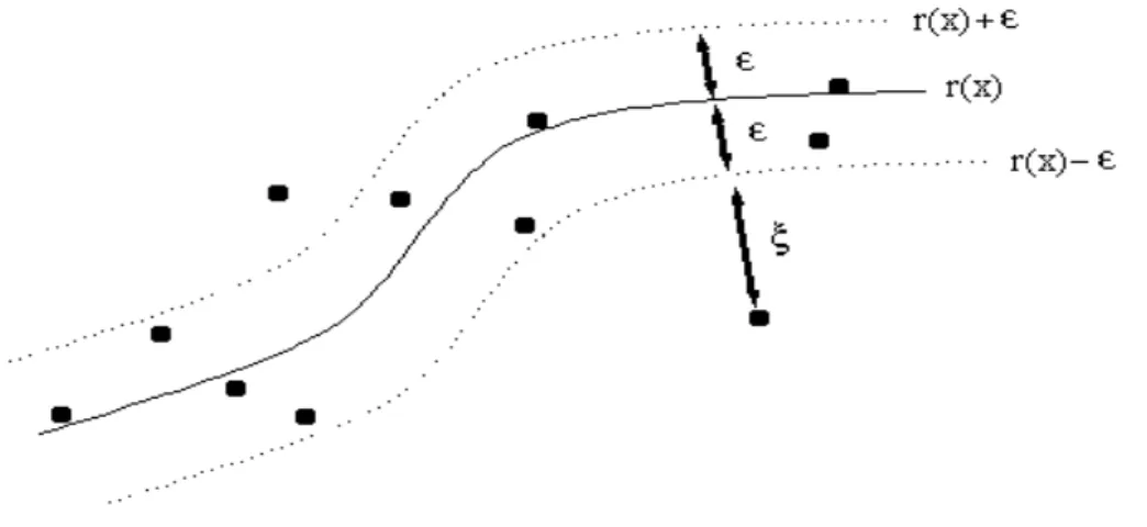
(2.5)

But, unfortunately, some data may lie outside of this epsilon tube due to noise or outliers making these constraints too strong and impossible to fulfil. In this case Vapnik suggests to introduce so called slack variables

ξ

i

,

ξ

i* . These variables measure the distance between the observation and the

ε

tube (see the example in Figure 2.1). The distance between the observation and the

ε

and

ξ

i

,

ξ

i* is illustrated by the following example: imagine you have a great confidence in your measurement process, but the variance of the measured phenomena is large. In this case,

ε

has to be chosen a priori very small while the slack variables

ξ

i

,

ξ

i* are optimised and thus can be large. Remember that inside the epsilon tube

([f(x,y)-

ε

,

f(x,y)+

ε

])

cost function is zero.

Figure 2.1. Support vector regression. Explanation of the

ε

–tube and slack variables.

Note that by introducing the couple (

ξ

i

,

ξ

i*) the problem has now 2n unknown variables. But these variables are linked since one of the two values is necessary equals to zero. Either the slack is positive

(

ξ

i*

= 0)

or negative

(

ξ

i

= 0).

Thus,

Z

i

∈

[f(x,y)-

ε

-

ξ

i

, f(x,y)+

ε

+

ξ

i*

]

.

Now, we are looking for a solution minimising at the same time its complexity (measured by

||w||

2) and its prediction error (represented by max

(

ξ

i

,

ξ

i*

)=

ξ

i

+

ξ

i* ) . In this case, let us introduce a user specified trade off parameter C between these two contradictory objectives. That leads us to the following problem:

minimise

1

2

|| ||

(

)

*

ω

2

ξ

ξ

1

+

+

=

∑

C

_{i i} i n (2.6)

subject to

for i = 1,...n

f x y

Z

f x y

Z

i i i i i i i i i i i

( ,

)

( ,

)

,

* *

−

−

≤

−

+

−

≤

≥









ε

ξ

ε

ξ

ξ ξ

0

2.3.2 Dual formulation

A classical way to reformulate a constraint based minimisation problem is to look for the saddle point of Lagrangian L:

∑

∑

∑

∑

= = = =

+

−

+

+

−

−

+

+

−

−

+

+

=

n i n i i i i i i i i i i i n i n i i i i i i i i i

Z

y

x

f

y

x

f

Z

C

w

w

L

1 1 * * * * 1 1 * 2 *

)

(

)

)

,

(

(

)

)

,

(

(

)

(

||

||

2

1

)

,

,

(

ξ

η

ξ

η

ξ

ε

α

ξ

ε

α

ξ

ξ

α

ξ

ξ

where

α α η η

_i

,

_i*

,

_i

,

_i* are Lagrangian multipliers associated with the constraints. They can be roughly interpreted as a measure of the influence of the constraints in the solution. A solution with

α

_i

=

α

_i*

=

0

can be interpreted as “the corresponding data point has no influence on this solution”.

At the minimum the derivative of the Lagrangian equals to zero (Kuhn-Tacker conditions). Thus it can be checked that:

w

x y

C

C

k i i k i i i n i i i i

=

−

= −

= −

=

∑

(

*

)

( ,

)

* *

α

α ϕ

η

α

η

α

for k = 1,... m

for i = 1,..., n

for i = 1,..., n

1

These variables can be removed from the original formulation of the minimisation problem to get the dual formulation of the problem:

maximise -

1

2

subject to

for

= 1,... m

for i,... n

i=1 n

(

)

( ,

)

(

,

) (

)

(

)

(

)

(

)

( ,

)

,

* * * * * *

α

α

ϕ

ϕ

α

α

ε α

α

α

α

α

α

α α

i i k i i k j j k m j j j n i n i i i i i i i n i n i i j i i j i i

x y

x

y

Z

K x y

K

C

−









−

−

+

+

−

−

=

≤

≤









= = = = =

∑

∑

∑

∑

∑

∑

1 1 1 1 1

0

0

(2.8)

This problem is untractable because of functions

ϕ

.

2.3.3 The nature of the solution

Now we are going to solve the problem (2.6) without specifying functions

ϕ

k. To do so it is necessary

to choose

ϕ

k such that:

(

)

ϕ

k

ϕ

k m i i k j j i i j j

x y

x

y

G x y

x

y

=

∑

=

1

( ,

)

(

,

)

( ,

), (

,

)

This is the case in reproducing kernel Hilbert space, where G is the reproducing kernel. Functions

ϕ

k

f x y

v G x y

_i

x y

_{i i j}

K x y

_j j m i n ∧ = =

=

∑

+

∑

( , )

(( , ), ( ,

))

β

( , )

1 1 (2.9) with

v

i

=

(

i

−

i

)

*

α

α

. Note that function

ϕ

k has disappeared. This solution only depends on the

kernel function

G

. Note also that here at least one of alphas is equalled to zero depending of the observed value

Z

i , above or under the

ε

-tube.

Remark: the solution proposed in equation (2.9) is the same as the regression spline and kriging estimates (since they are positive definite and reproducing kernels can be interpreted as covariance function (Wahba 1990). The difference between these methods lies in the underlying hypotheses and thus in the way weights in (2.9) are estimated. In the SVR framework the regularisation is not performed on

v

but on the representation of the function in some feature space. This is a way to define a regularisation principle that guarantees an explicit bound on the IPE error. From the practical point of view, due to L1 type minimisation, many of the

v

i can be either zero or C.

v

i is zero when associated measurement point

lies within the ε-tube and thus has no influence on the estimation. This point is useless for the estimation and can be removed without changing the result.

v

i is equals to C when the associated measurement point

is too far from the ε-tube. In this case, the influence of the point is bounded at C. Another way to formulate this remark is to establish the link between SVR and sparse approximation (Girosi 1998).

2.4 Practical implementation of the solution

2.4.1 Practical formulation of the QP problem

The minimisation problem (2.8) is a quadratic programming (QP) problem with very specific box constraints. It has got 2n unknown variables

(

α α

*i

,

i

)

for only n data points. Thus, it is necessarily very

badly conditioned. This problem can be written in the following way:

min[

' '

]

'

1

2

0

0

α α

α

α

α

H

b

d

C

−

=

≤ ≤

















(2.10) where: •

α

=

(

α

*

,...,

α

*

,...,

α α

*

;

,...,

α

,...,

α

)

1 i n 1 i n - is the 2n-dimensional vector to be found

•

H

is a symmetric matrix such that

H

G

G

G

G

=

−

−













, where

G

denotes the kernel

matrix such that Gi,j = G((xi,yi,),(xj,yj))

•

b

=

(

z

1

−

ε

1

,...,

z

i

−

ε

i

,...,

z

n

−

ε

n

,

− −

z

1

ε

1

,...,

− −

z

i

ε

,...

− −

z

n

ε

n

)

•

d

j

=

(

K

j

(

x y

1

,

1

),...,

K

j

(

x

n

,

y

n

),

−

K

j

(

x y

1

,

1

),...,

−

K x

j

(

n

,

y

n

))

The main difficulty of this QP problem lies in its dimension. For 1000 data points the problem to be solved is of dimension 2000 that makes it intractable for most of the commercial optimisation software.

Equality constraints are not too complex since they are very few. Box constraints are also rather simple but there are many of them (4n). This suggest to use a specific algorithm taking into account the specificity of the box constraints.

2.4.2 Kernel choice

A typical practical choice for the kernel is the Gaussian Kernel:

G x y

i i

x

j

y

j

x

x

y

y

i j i j

((

,

), (

,

))

=

exp

−

(

−

)

+

(

−

)

2 2 2

σ

where

σ

denotes the bandwidth of the kernel.

In this case

j=1

and the trend function

K

is a constant.

2.4.3 Hyper parameters

For practical implementation the hyper parameters of the method have to be tuned. These parameters are the following:

•

C

: although often recommended as very large, geostatistical applications show a great deal of dependence on this parameter. It has to be tuned carefully.

•

ε

i : if no additional information is available the easiest way to tune it is to put it small and equal

for all data points. See below details on influence of the epsilon on training and mapping.

•

σ

:

the bandwidth of kernel. Here again the IPE of the proposed solution is very sensitive to this parameter. More generally, the performance of the solution is sensitive to the distance matrix used in the kernel

• preconditioning matrix H: because H is very ill conditioned, it is recommended to improve its conditioning by adding some quantity on its diagonal (regularisation). It looks that the solution is quiet insensitive to this treatment.

3. SOFTWARE DESCRIPTION

For the present study Matlab programs for the support vector regression were used. These programs have been developed by S. Canu. For the exploratory data analysis, variography and presentation of the results Geostat Office software was used (Kanevski et al. 1999c).

4. CASE STUDY

In the present case study data on the most contaminated Briansk region of Russia by Chernobyl radionuclide Cs137 are used. This data set is a well known since it has been studied extensively with the help of different methods including geostatistics, artificial neural networks and wavelets. Data represent variability at several scales. They are spatially nonstationary.

The generic procedure for the spatial data analysis, modelling and presentation was described in [Kanevski et al. 1999c]. The same procedure is adapted here with SVR instead of other regression models. Basic steps deal with exploratory statistical analysis, monitoring network qualitative and quantitative description, comprehensive structural analysis – variography, regression model development testing, validation and decision oriented mapping.

The present data are rather typical for environmental and pollution studies. Data are positively skewed and there are some hot spots with rather high concentrations. Data were described in detail in several previous publications [Kanevski et al 1996]. Only short (geo)statistical description of data are presented below.

The original data base containing 665 measurements was split into 2 parts with different proportions several times. Data sets were prepared for the numerical experiments with geostatistical models and artificial neural networks. Basically different algorithms have to be used for data splitting including algorithms of spatial declustering. In the present study only the results of particular splitting of data into 200 training data and 465 testing data was presented. Influence of splitting is a topic of the research under progress.

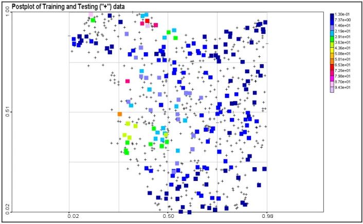
Postplots of training and testing data are shown in Figure 3.1. Very often input space is transformed or projected into some box region. There are some numerical advantages of such transformations. Other considerations deal with modification of spatial correlation structures: simpler spatial structures (e.g. less anisotropic) can be modelled with less number of Support Vectors and solutions can be more robust with better generalisation.

In our case we have transformed original [Xmin Xmax]x [Ymin Ymax] co-ordinates into [0,1]x[0,1] 2D

box. All results will be presented in this transformed space.

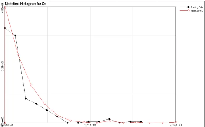
Histograms of raw training and testing data sets are presented in Figure 3.2. There are 7 measurements with rather high values of contamination.

Figure 3.2 Histograms for Training and Testing data.

4.2 Structural analysis. Variography

Structural analysis - Variography – is a key phase of any geostatistical analysis. Variography is related to the quantitative description of spatial continuity of the phenomena under study.

There are two major parts of the variography: experimental variography 1) calculation of experimental based on data variograms,

2) modelling, which in fact is fitting of theoretical models to the experimental variograms.

In general both exploratory and theoretical parts of variography need deep expert knowledge and experience. Details on variography and related topics along with examples of interpretation can be found in geostatistical books (see refnces).

Semivariogram (variogram) is the basic tool of the spatial structural analysis variography. Theoretical formula for the variogram (under the intrinsic hypotheses) is following

Empirical estimate of the semivariogram

Where

N(h) –

number of pairs separated by vector h.

{

}

{

(

)

}

γ

( , )

x h

=

1

( )

x

−

(

x

+

h

)

=

( )

x

−

(

x

+

h

)

=

γ

( )

h

2

1

2

2

Var Z

Z

E Z

Z

(

)

γ

∧ =

=

∑

−

+

( )

( )

( )

(

)

( )

h

h

x

x

h

h

1

2

2 1

N

i

Z

i

Z

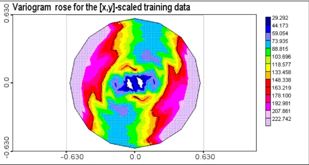
i N

Figure 3.3. Experimental variogram rose for the training data.

Experimental (estimated using data) variogram rose for testing data is presented in Figure 3.4. There are some differences in anisotropy for the spatial correlation between training and testing data.

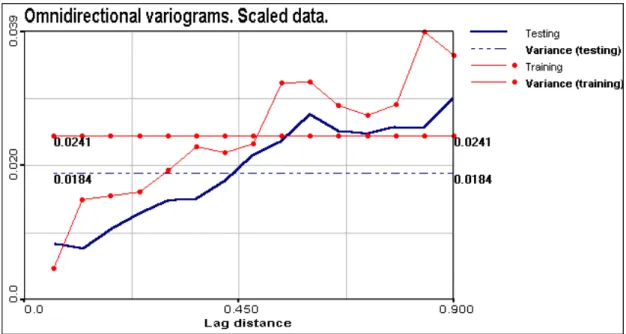
Figure 3.5. Omnidirectional variograms for training and testing data. A priori variances are indicated as well.

Structural analysis (variography) is a very important exploratory phase of spatial data. It describes relationships between stochastic and spatially structured information (by comparing nugget and sill). Anisotropic spatial correlation structures can be evaluated. Variogram tools are used to check second order stationarity and intrinsic hypotheses.

NB! In order be correct both data sets should be generated from the same (unknown) probability distribution functions – in general joint distribution functions. In the present research mainly 1st (univiate pdf) and 2nd (variograms) order moments are considered. From this point of view FINITE data sets (training, testing and in general validation) should have the same univariate pdf (histograms) and variograms. Basically, from one realisation and with finite data sets it is very difficult (possible?), to make such decisions. In the present case study variability (described e.g. by sill values) is higher for more comprehensive testing data set.

In the following sections variography is used as a tool to qualify the performance of SVR mapping.

4.3 SVR training

In accordance with statistical learning theory SVR are the powerful machines for function modelling based on finite number of data. Most of the parameters are tuned automatically during SVR training. Nevertheless, there are 3 so-called hyper parameters which have to be tuned a priori: epsilon value (coming from

ε

-insensitive cost function),

C

parameter and kernel bandwidth

σ

.

There are different approaches how to choose the optimal parameters of the SVR. In the present study testing/validation data set is used.

The basic idea is to extract from the data all “useful” information and to develop optimal model. “Useful” here means spatially structured information. As a quantitative measure statistical analysis and variography of the SVR results and residuals are used.

Input (X,Y) and output (Z) space of training data can be characterised with several simple parameters useful for the understanding and selection of the SVR parameters:

Input space: minimum distance between points Rmin= 0.0036, maximum distance between points Rmax = 1.2; averaged distance between points Rave = 0.066.

Output space: Large RCL and small RCS radii of spatial correlation ranges from 0.12 up to almost the

value distances at which variogram reaches a sill can be used. Omnidirectional variogram for training data reaches a sill value at distance 0.5.

Variability of data: nugget effect corresponding to error measurements and small scale variability that is not resolved by monitoring network. Sqrt(estimated nugget) = 0.03; sill (plato = a priori variance) of the training data variogram = 0.0241.

In the present study understanding of input and output space units and characteristic parameters is used to select and explain the “best” region of hyper-parameters. The same epsilon value was used for all data points. Basically, varying epsilon value from point to point it is possible to take into account spatially distributed local variability. From another side, if epsilon is too big – compared with data variance [sqrt(sill)], it is clear that all data lye in the epsilon tube and the solution is a kind of data averaging (with bias, depending on data). The transition zone is between sqrt(nugget) and sqrt(sill). Let us remind that sqrt function is applied because we are working with L1 loss function.

It seems also reasonable that kernel bandwidth is related to spatial variability of data described by variogram structures. It was shown (Kanevski et al. 1996) that with multilayer perceptrons and with RBF ANN (Kanevski et al. 1999d) different information can be extracted from data with solutions varying from overfitting to oversmoothing (trend extraction). The anisotropy can also be taken into account by three different ways: 1) data preprocessing – from anisotropic spatial correlations to isotropic (when possible); 2) by modifying SVR kernel from isotropic to anisotropic (covariance matrix – Mahalanobis distance in the input space) and 3) by local adaptation of the SVR. The last case can be very computationally demanding.

Some results of the training when trying to tune hyper parameters by using testing data set are presented below.

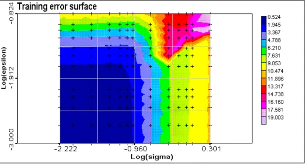
The main results of training are presented as the training (Figure 6) and testing (Figure 7) error surfaces and as the Number of SV surface (Figure 8). C parameter was fixed at 10. Some typical one dimensional cross-sections are presented in Figures 9-10.

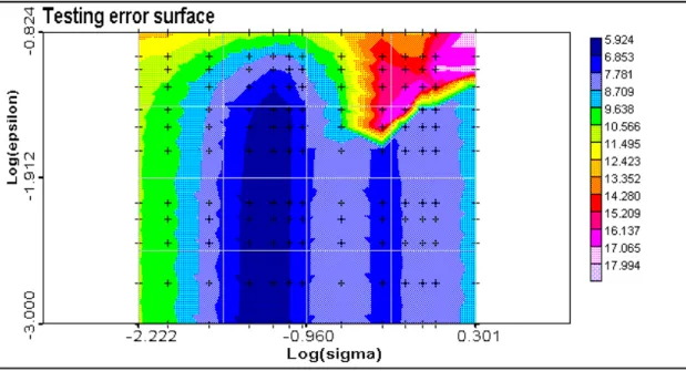
Figure 4.2. Testing error surface: testing error versus kernel bandwidth and epsilon. C=10.

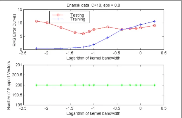
Figure 4.4. Training and testing error curves (above) and Number of Support Vectors at epsilon=0.0 and “optimal” kernel bandwidth s= 0.065. C =10.

Figure 4. Training and testing error curves (above) and Number of Support Vectors at epsilon = 0.02 and kernel bandwidth s= 0.065. C =10.

Some conclusions about SVR training phase can be summarised as follows:

C parameter. If C parameter is not too small (close to the variability of data) it does not significantly influence error curves. It means that practically it is not necessary to put it as a very large vakue. This is important because of numerical stability. Most of the results are presented with C=10 (before training measurement data were rescaled and the variability of scaled data ranges from 0 to 1).

Training and testing error surfaces. At fixed small epsilon value with increasing kernel bandwidth error curves can be easily understood as running from overfitting to oversmoothing region. Up to some epsilon value it does not influence training and testing errors. This level is almost the same both for training and testing error surfaces and seems to be related to the nugget effect (square root of the nugget). After this value the epsilon-tube is covering spatially structured information and the model is bad and highly biased. In general, behaviour of training and testing error surfaces is similar except some region on testing error surface where error minimum is achieved.

Number of support vectors. Of course, at epsilon equals to zero all data points are support vectors despite of kernel bandwidth. Number of SV curves change behaviour with increasing of epsilon. There is a clear region with minimum of SV. This minimum is decreasing with increase of epsilon: less support vectors is necessary to have rough solutions. Partly region with minimum of SV corresponds to the minimum of testing error. This is an interesting and useful property of SVR. The universality of this behaviour should be tested more. With a fixed epsilon value qualitatively the behaviour of the number f Support Vectors is similar to the one found in environmental data classification problems (Kanevski et al. 1999b). Increase of the kernel bandwidth simplifies the kernel function and more support vectors are necessary to reproduce even simple solutions.

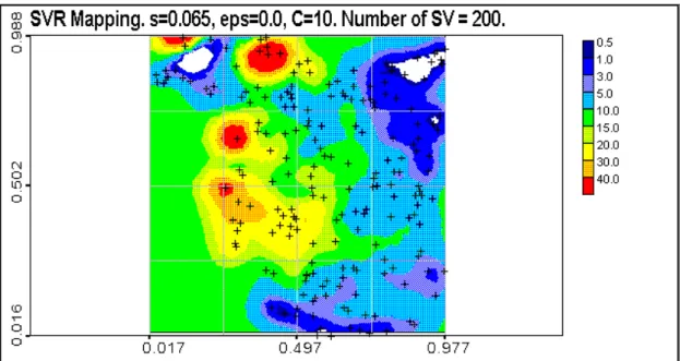
4.4 SVR mapping

Let us consider some results of the SVR mapping. Maps with different hyper parameters are presented below, describing overfitting, “optimal” modeling and detrending (oversmoothing).

The objective of pollution mapping is to extract “useful” information from data, develop a model with good generalization ability. In terms of spatial statistics “useful” means spatially structured information. Spatial structures can be described by variograms. Therefore, to control the quality of mapping, variography of the residuals (both training and testing) and the results is performed. Of course, higher moments can be used to control the quality of the mapping, but it seems to be impractical.

Detrending – large scale or, in general, multiscale modeling. The problem is to develop non-linear robust model for the extraction “useful” information at some scales, leaving small scale variability. Powerful and flexible SVR is a good candidate. Moreover, in this case it is possible to derive robust model with a small number of support vectors.

Figure 4.6. SVR mapping at kernel bandwidth s= 0.065, C=10 and epsilon = 0.0. Number of support vectors NSV = 200 (all data).

Figure 4.7. SVR mapping at kernel bandwidth s= 0.065, C=10 and epsilon = 0.01. Number of support vectors NSV = 147. Comment: almost the same solution like in figure 4.25 but with less number of support vectors.

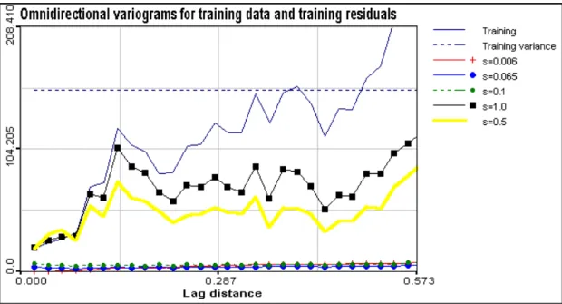
Figure 4.8. Omnidirectional variograms for training data and training residuals. at different kernel bandwidth and epsilon = 0.03, C1 = 10

Figure 4.9. Omnidirectional variograms. Training and testing residuals at different kernel bandwidth and epsilon = 0.03, C = 10.

Let us note that both training and testing variograms residuals demonstrate almost pure nugget effect (no spatial correlation) near optimal solution. Let us note that small scale variability in testing data described by nugget effect is higher than in training data.

Figure 4.10. SVR mapping at kernel bandwidth s= 0.065, C=10 and epsilon = 0.03. Number of support vectors NSV = 114.

The same hyper-parameters as in Figures 4.6, 4.7 but the epsilon value equals to the square root of nugget. This value is the biggest one recommended in the present study. Number of support vectors is almost half of the number of training data.

Figure 4.11. SVR detrending. Kernel bandwidth = 1.0 (length of the region under study) and epsilon value is about square root of nugget. Number of support vectors =125.

The idea was to extract large scale trends over the region with the minimum number of support vectors (that’s why epsilon value was taken as the biggest possible one). The efficiency of detrending can be analyzed with the help of variogram of the residuals.

Figure 4.12. Omnidirectional variograms for the results presented in Figure 4.30 with SVR detrending. There is a nice stationary variogram for the residuals. Excellent candidate for the development of SVRRK (Support Vector Regression Residual Kriging) models. (see Kanevsky et al 1996).

5. DISCUSSIONS AND CONCLUSIONS

The report presents the first study of Support Vector Regression (SVR) application to the environmental and pollution data mapping.

It was shown that using structural analysis to describe “useful” information in spatial data is very powerful approach.

The SVR was trained using learning data set and validated with testing data. Testing data set was used to tune hyper parameters of the SVR: C parameter, kernel bandwidth and epsilon. Besides, comprehensive structural analysis of raw data, the results and the residuals was carried out to:

1) exploratory raw data analysis and understanding,

2) control the performance of the SVR using variography of the results and the residuals.

It was shown that SVR mapping is powerful and very flexible approach enabling to extract information at different scales. By controlling hyper parameters it as possible to cover the whole range of model’s complexity from overfitting/interpolating data to large scale nonlinear detrending.

It seems natural to choose epsilon parameter corresponding to small scale variability (in general, small scale variability+error measurements) described by nugget effect (less than). In case of epsilon equals to zero all data are support vectors. With increasing epsilon value the number of support vectors decreases monotonically. When epsilon is higher than square root of nugget the developed model is biased (in our case overestimation) was obsved.

When C parameter is much larger than the variability of data used for SVR training it has no significant influence on the results. Thus, reasonable selection of C can be in the range of the training data variability.

Kernel bandwidth has very important influence on the results of mapping. After appropriate selection of the C parameter and epsilon, kernel bandwidth controls the behavior of the solution – from overfitting to oversmoothing. In the region of optimal kernel bandwidth (minimum testing error) the number of support vectors is minimum as well.

At present, the challenge for the SVR application to environmental and pollution data analysis, modelling and presentation deals with probabilistic mapping – developing of models and mapping of local probability density functions. The counterparts in geostatistics are disjunctive and indicator kriging.

6. ACKNOWLEDGEMENTS

The work was supported in part by INTAS grants 31726 and 99. The main part of the work was carried out during visit of M. Kanevski at INSA (Rouen, 1999), IDIAP (Martigny, 1999-2000) and University of Lausanne (2000) as an invited Professor. Authors thank to Geostat Office group for the kind possibility to use Geostat Office software.

7. REFERENCES

Canu S. and M. Kanevski. Environmental and Pollution Data Mapping with Support Vector Regression. INSA Rouen Research Report, July 1999. 34 pp.

Cherkassky V and F. Mulier. Learning from data. Wiley Interscience, N.Y. 1998, 441 p.

Deutsch C.V. and A.G. Journel. GSLIB. Geostatistical Software Library and User’s Guide. Oxford University Press, New York, 1997.

Girosi F. An equivalence between sparse approximation and support vector machines. Neural Computation, 10(1), pp. 1455-1480, 1998.

Goovaerts P. Geostatistics for Natural Resources Evaluation. Oxford University Press, New York, 1997. Kanevski M., Arutyunyan R., Bolshov L., Demyanov V., Maignan M. Artificial neural networks and spatial estimations of Chernobyl fallout. Geoinformatics. Vol.7, No.1-2, 1996, pp.5-11.

Kanevski M., N. Gilardi, M. Maignan, E. Mayoraz. Environmental Spatial Data Classification with Support Vector Machines. IDIAP Research Report. IDIAP-RR-99-07, 24 p., 1999a. (www.idiap.ch) Kanevski M, V. Demyanov, S. Chernov, E. Savelieva, A. Serov, V. Timonin, M. Maignan. Geostat Office for Environmental and Pollution Spatial Data Analysis. Mathematische Geologie, N3, April 1999c, pp. 73-83.

Kanevski M. Spatial Predictions of Soil Contamination Using General Regression Neural Networks. Int. J. on Systems Research and Information Systems, Volume 8, number 4. Special Issue: Spatial Data: Neural nets/Statistics. Guest Editors Dr. Patrick Wong and Dr. Tom Gedeon.Gordon and Breach Science Publishers PP.241-256. 1999.

Smola A.J., and B. Scholkopf. A Tutorial on Support Vector Regression. NeuroColt2 technical Reports Series, NC2-TR-1998-030, October 1998.

Vapnik V. Statistical Learning Theory. John Wiley & Sons, 1998.

Wahba G. Spline Models for Observational Data. No. 59 in regional conference series in applied mathematics, SIAM Philadelphia, Pennsylvania 1990.