Air Force Institute of Technology
AFIT Scholar
Theses and Dissertations Student Graduate Works
9-13-2012
Utilizing Graphics Processing Units for Network
Anomaly Detection
Jonathan D. Hersack
Follow this and additional works at:https://scholar.afit.edu/etd
Part of theInformation Security Commons
This Thesis is brought to you for free and open access by the Student Graduate Works at AFIT Scholar. It has been accepted for inclusion in Theses and Dissertations by an authorized administrator of AFIT Scholar. For more information, please [email protected].
Recommended Citation
Hersack, Jonathan D., "Utilizing Graphics Processing Units for Network Anomaly Detection" (2012).Theses and Dissertations. 1119.
UTILIZING GRAPHICS PROCESSING UNITS FOR NETWORK
ANOMALY DETECTION
THESIS
Jonathan D. Hersack, CIV AFIT/GCO/ENG/12-24
DEPARTMENT OF THE AIR FORCE AIR UNIVERSITY
AIR FORCE INSTITUTE OF TECHNOLOGY
The views expressed in this thesis are those of the author and do not reflect the official policy or position of the United States Air Force, the Department of Defense, or the United States Government.
This material is declared a work of the U.S. Government and is not subject to copyright protection in the United States.
AFIT/GCO/ENG/12-24
UTILIZING GRAPHICS PROCESSING UNITS FOR NETWORK
ANOMALY DETECTION
THESIS
Presented to the Faculty
Department of Electrical and Computer Engineering Graduate School of Engineering and Management
Air Force Insitute of Technology Air University
Air Education and Training Command in Partial Fulfillment of the Requirements for the Degree of Master of Science in Cyber Operations
Jonathan D. Hersack, B.S.C.S.E. CIV
AFIT/GCO/E~G/12-24
UTILIZING GRAPHICS PROCESSING UNITS FOR NETWORK
ANOMALY DETECTION
Jonathan D. Hcr..ad ... B.S.C.S.E. CIV
Approved:
, lu;.f
11.
L<--v
ltichael R. Grimaila. PhD, CISM, CISSP (:\1cmber)
2Cf
,r/1/(r
1'2.
DateAbstract
Network intrusion detection signatures are often outdated as new attacks are developed more quickly than signatures. Machine learning anomaly-based network intrusion detection methods provide the ability to detect unknown attacks but require significantly more processing time than signature detection methods. The availability of Graphics Processing Units (GPUs) in many personal computers leads to a potential solution for a scalable, cost-e↵ective network anomaly detection system. This research explores the benefits of using commonly-available graphics processing units (GPUs) to perform classification of network traffic using supervised machine learning algorithms. Two full factorial experiments are conducted using a NVIDIA GeForce GTX 280 graphics card. The goal of the first experiment is to create a baseline for the relative performance of the CPU and GPU implementations of Artificial Neural Network (ANN) and Support Vector Machine (SVM) detection methods under varying loads. The goal of the second experiment is to determine the optimal ensemble configuration for classifying processed packet payloads using the GPU anomaly detector. The configurations include three base classifier configurations and two ensemble combination methods.
Experimental results show that the GPU implementation of the anomaly-based network intrusion detection system provides significant training and testing speedups over the CPU implementation for the Network Security Laboratory Knowledge Discovery and Data mining (NSL-KDD) dataset as well superior scaling across the load sizes evaluated. The GPU ANN achieves speedups of 29x over the CPU ANN. The GPU SVM detection method shows training speedups of 85x over the CPU. The GPU ensemble classification system provides accuracies of 99% when classifying network payload traffic, while achieving speedups of 2-15x over the CPU configurations. These results indicate the the
Acknowledgements
I would like to thank my advisor, Dr. Barry Mullins, for his encouragement throughout the research process. I would also like to thank Dr. Rusty Baldwin for his advice and feedback.
Table of Contents Page Abstract . . . iv Dedication . . . v Acknowledgements . . . vi List of Figures . . . x
List of Tables . . . xii
1 Introduction . . . 1
1.1 Motivation . . . 1
1.2 Overview and Goals . . . 2
1.3 Thesis Layout . . . 3
2 Background and Related Work . . . 4
2.1 Intrusion Detection . . . 4
2.1.1 Development of the Intrusion Detection System . . . 4
2.1.2 Misuse Detection . . . 5
2.1.3 Anomaly Detection . . . 5
2.1.4 Common IDS Techniques . . . 6
2.2 Machine Learning . . . 7
2.2.1 Learning Types . . . 7
2.2.2 Supervised Learning . . . 8
2.2.3 Cross-Validation . . . 8
2.3 Selected Machine Learning Techniques . . . 9
2.3.1 Support Vector Machines . . . 9
2.3.2 Theoretical Basis for SVM . . . 10
2.3.3 Artificial Neural Networks . . . 11
2.3.4 Feed-Forward Neural Network . . . 13
2.3.5 Training Feed-Forward Neural Networks . . . 14
2.3.6 Ensembles . . . 15
2.4 Related Machine Learning IDS Work . . . 16
2.5 Graphics Processing Units . . . 17
2.5.1 Graphical Processing Units . . . 17
2.5.2 General Purpose Computing on GPU . . . 18
2.5.3 CUDA Model . . . 19
2.5.5 CUDA Compute Capability . . . 25
2.6 Related GPGPU Work . . . 26
2.7 Machine Learning Implementations . . . 27
2.7.1 LIBSVM . . . 27 2.7.2 GTSVM . . . 28 2.7.3 LIBCUDANN . . . 30 2.8 Summary . . . 31 3 Methodology . . . 32 3.1 Problem Definition . . . 32 3.2 System Boundaries . . . 33 3.3 System Services . . . 35 3.4 Workload . . . 35
3.4.1 NSL-KDD Evaluation Workload Creation . . . 36
3.4.2 McPAD Evaluation Workload Creation . . . 38
3.5 Performance Metrics . . . 40 3.6 System Parameters . . . 41 3.7 Factors . . . 44 3.7.1 System Factors . . . 44 3.7.2 Workload Factors . . . 46 3.8 Evaluation Technique . . . 47 3.9 Experimental Design . . . 47 3.10 Methodology Summary . . . 49
4 Results and Analysis . . . 50
4.1 Results and Analysis of Experiment 1 . . . 50
4.1.1 Analysis of Di↵erences in Execution Time . . . 50
4.1.1.1 Statistical Significance of Di↵erences in Execution Time 51 4.1.1.2 Comparison of ANN Implementations . . . 52
4.1.1.3 Impact of Parameter Sets On SVM Implementations . . . 55
4.1.1.4 Comparison of CPU and GPU SVM Training Times . . . 59
4.1.1.5 Comparison of CPU and GPU SVM Testing Times . . . 61
4.1.2 Analysis of Classifier Accuracy . . . 62
4.2 Results and Analysis of Experiment 2 . . . 65
4.2.1 Impact of Datasets and Cluster Levels on Classifier Execution Times 66 4.2.2 Analysis of Di↵erences in Execution Times . . . 67
4.2.2.1 Analysis of Di↵erences in ANN Implementations . . . . 67
4.2.2.2 Analysis of Di↵erences in SVM Implementations . . . . 71
4.2.3 Analysis of Ensemble Accuracy . . . 74
4.2.3.1 Impact of Machine Learning Algorithm on Accuracy . . 75
4.3 Analysis Highlights . . . 81
4.4 Summary . . . 82
5 Conclusions . . . 83
5.1 Conclusions of Research . . . 83
5.1.1 Goal 1: Determine the Relative Accuracy of the GPU Machine Learning Anomaly Detection Algorithms . . . 83
5.1.2 Goal 2: Measure the Relative Performances of the CPU and GPU Implementations of the Anomaly Detector . . . 83
5.1.3 Goal 3: Determine the Relative Accuracy of Varying Ensemble Configurations . . . 84
5.2 Impact of Research . . . 85
5.3 Recommendations for Future Work . . . 85
Appendix A: Supplemental Data for Experiment 1 . . . 87
Appendix B: Experimental Data for Experiment 1 . . . 91
Appendix C: Supplemental Data for Experiment 2 . . . 102
Appendix D: Experimental Data for Experiment 2 . . . 114
List of Figures
Figure Page
2.1 Support Vector Example . . . 9
2.2 An Artificial Neuron . . . 12
2.3 Example Multilayer ANN . . . 13
2.4 CPU Control versus GPU Control . . . 18
2.5 CUDA Thread Hierarchy . . . 19
2.6 Branching Example . . . 20
2.7 CUDA Thread Block Scaling . . . 21
2.8 CUDA Kernel Execution . . . 22
2.9 CUDA Memory Hierarchy . . . 23
2.10 CUDA Application Compilation and Linking . . . 25
2.11 GTSVM Clustering Example . . . 30
3.1 GPU-Accelerated Network Intrusion Detection System . . . 34
4.1 ANN Training Times versus Dataset Size . . . 54
4.2 ANN Testing Times versus Dataset Size . . . 54
4.3 CPU SVM Training Times versus Dataset Size . . . 56
4.4 CPU SVM Testing Times versus Dataset Size . . . 57
4.5 GPU SVM Training Times versus Dataset Size . . . 58
4.6 Average Accuracies for All Classifiers . . . 64
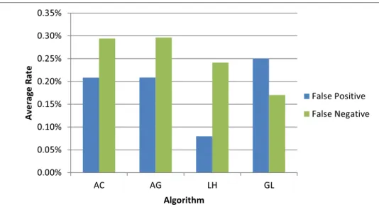
4.7 Average False Positive Rates . . . 65
4.8 Average False Negative Rates . . . 65
4.9 Mean Training Times of ANNs for 40 Cluster Datasets . . . 68
4.13 Mean Training Times of SVMs for 40 Cluster Datasets . . . 71
4.14 Mean Training Times of SVMs for 160 Cluster Datasets . . . 72
4.15 Mean Testing Times of SVMs for 40 Cluster Datasets . . . 73
4.16 Mean Testing Times of SVMs for 160 Cluster Datasets . . . 73
4.17 Average Accuracies for 40 Cluster Voting Ensembles . . . 77
4.18 Average Accuracies for 40 Cluster Final Classifier Ensembles . . . 78
4.19 Average Accuracies for All 40 Cluster Ensembles . . . 79 4.20 False Positive and Negative Rates for 5 BC Final Classifier 40 Cluster Ensembles 81
List of Tables
Table Page
2.1 CUDA Memory Types . . . 24
3.1 Traffic Distribution for NSL-KDD Dataset . . . 37
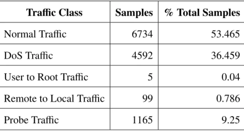
3.2 Traffic Distribution for NSL-KDD 10% Subset . . . 38
3.3 Input File Distribution for McPAD 60% Subset . . . 40
3.4 Specifications for PNY GeForce GTX 280 . . . 43
3.5 Factors and Levels for NSL-KDD Workload . . . 44
3.6 Factors and Levels for McPAD Workload . . . 44
3.7 Values ofvfor Base Classifier Datasets . . . 45
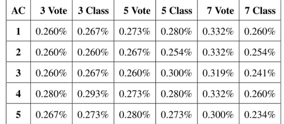
4.1 Di↵erence in Mean Testing Time (ms) for the GPU Support Vector Machines . 51 4.2 Mean Execution Times for CPU ANN (AC) . . . 52
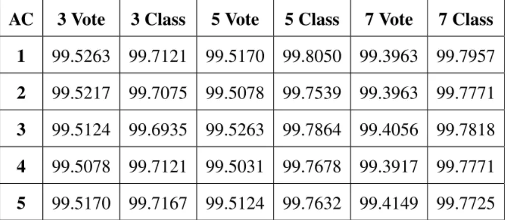
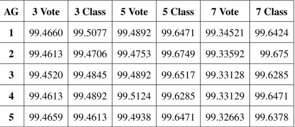
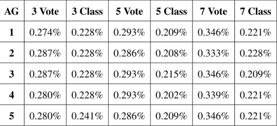
4.3 Mean Execution Times for GPU ANN (AG) . . . 52
4.4 Ratio of CPU ANN Times to GPU ANN Times (AC/AG) . . . 53
4.5 Mean Execution Times for CPU SVM-High (LH) . . . 55
4.6 Mean Execution Times for CPU SVM-Low (LL) . . . 55
4.7 Ratio of CPU SVM-L Times to CPU SVM-H Times (LL/LH) . . . 56
4.8 Ratio of GPU SVM-H Times to GPU SVM-L Times (GH/GL) . . . 58
4.9 Mean Execution Times for GPU SVM-High (GH) . . . 59
4.10 Mean Execution Times for GPU SVM-Low (GL) . . . 59
4.11 Ratio of CPU SVM-H Times to GPU SVM-H Times (LH/GH) . . . 60
4.12 Ratio of CPU SVM-L Times to GPU SVM-H Times (LL/GH) . . . 60
4.13 Ratio of CPU SVM-H Times to GPU SVM-L Times (LH/GL) . . . 61
A.1 Traffic Distribution for NSL-KDD 20% Subset . . . 90
A.2 Traffic Distribution for NSL-KDD 30% Subset . . . 90
B.1 Training Times (s) for CPU ANN . . . 91
B.2 Training Times (s) for GPU ANN . . . 91
B.3 Training Times (s) for GPU SVM-High . . . 92
B.4 Training Times (s) for CPU SVM-High . . . 92
B.5 Training Times (s) for GPU SVM-Low . . . 92
B.6 Training Times (s) for CPU SVM-Low . . . 93
B.7 Testing Times (ms) for CPU ANN . . . 93
B.8 Testing Times (ms) for GPU ANN . . . 93
B.9 Testing Times (ms) for GPU SVM-High . . . 94
B.10 Testing Times (ms) for CPU SVM-High . . . 94
B.11 Testing Times (ms) for GPU SVM-Low . . . 94
B.12 Testing Times (ms) for CPU SVM-Low . . . 95
B.13 Accuracies for CPU ANN . . . 95
B.14 Accuracies for GPU ANN . . . 95
B.15 Accuracies for GPU SVM-H . . . 96
B.16 Accuracies for CPU SVM-H . . . 96
B.17 Accuracies for GPU SVM-L . . . 96
B.18 Accuracies for CPU SVM-L . . . 97
B.19 False Positive Rates for CPU ANN . . . 97
B.20 False Positive Rates for GPU ANN . . . 97
B.21 False Positive Rates for GPU SVM-High . . . 98
B.22 False Positive Rates for CPU SVM-High . . . 98
B.23 False Positive Rates for GPU SVM-Low . . . 98
B.25 False Negative Rates for CPU ANN . . . 99
B.26 False Negative Rates for GPU ANN . . . 99
B.27 False Negative Rates for GPU SVM-High . . . 100
B.28 False Negative Rates for CPU SVM-High . . . 100
B.29 False Negative Rates for GPU SVM-Low . . . 100
B.30 False Negative Rates for CPU SVM-Low . . . 101
D.1 Training Times (s) for CPU ANN 40 Cluster Datasets . . . 114
D.2 Training Times (s) for GPU ANN 40 Cluster Datasets . . . 114
D.3 Training Times (s) for CPU SVM 40 Cluster Datasets . . . 115
D.4 Training Times (s) for GPU SVM 40 Cluster Datasets . . . 115
D.5 Training Times (s) for CPU ANN 160 Cluster Datasets . . . 115
D.6 Training Times (s) for GPU ANN 160 Cluster Datasets . . . 116
D.7 Training Times (s) for CPU SVM 160 Cluster Datasets . . . 116
D.8 Training Times (s) for GPU SVM 160 Cluster Datasets . . . 116
D.9 Testing Times (ms) for CPU ANN 40 Cluster Datasets . . . 117
D.10 Testing Times (ms) for GPU ANN 40 Cluster Datasets . . . 117
D.11 Testing Times (ms) for CPU SVM 40 Cluster Datasets . . . 118
D.12 Testing Times (ms) for GPU ANN 40 Cluster Datasets . . . 118
D.13 Testing Times (ms) for CPU ANN 160 Cluster Datasets . . . 118
D.14 Testing Times (ms) for GPU ANN 160 Cluster Datasets . . . 119
D.15 Testing Times (ms) for CPU SVM 160 Cluster Datasets . . . 119
D.16 Testing Times (ms) for GPU SVM 160 Cluster Datasets . . . 119
D.17 Accuracies for CPU ANN Ensembles 40 for Cluster Datasets . . . 120
D.18 Accuracies for GPU ANN Ensembles for 40 Cluster Datasets . . . 120
D.21 Accuracies for CPU ANN Ensembles for 160 Cluster Datasets . . . 121
D.22 Accuracies for GPU ANN Ensembles for 160 Cluster Datasets . . . 121
D.23 Accuracies for CPU SVM Ensembles for 160 Cluster Datasets . . . 122
D.24 Accuracies for GPU SVM Ensembles for 160 Cluster Datasets . . . 122
D.25 False Positive Rates for CPU ANN Ensembles for 40 Cluster Datasets . . . 122
D.26 False Positive Rates for GPU ANN Ensembles for 40 Cluster Datasets . . . 123
D.27 False Positive Rates for CPU SVM Ensembles for 40 Cluster Datasets . . . 123
D.28 False Positive Rates for GPU SVM Ensembles for 40 Cluster Datasets . . . 123
D.29 False Positive Rates for CPU ANN Ensembles for 160 Cluster Datasets . . . . 124
D.30 False Positive Rates for GPU ANN Ensembles for 160 Cluster Datasets . . . . 124
D.31 False Positive Rates for CPU SVM Ensembles for 160 Cluster Datasets . . . . 124
D.32 False Positive Rates for GPU SVM Ensembles for 160 Cluster Datasets . . . . 125
D.33 False Negative Rates for CPU ANN Ensembles for 40 Cluster Datasets . . . 125
D.34 False Negative Rates for GPU ANN Ensembles for 40 Cluster Datasets . . . . 125
D.35 False Negative Rates for CPU SVM Ensembles for 40 Cluster Datasets . . . 126
D.36 False Negative Rates for GPU SVM Ensembles for 40 Cluster Datasets . . . . 126
D.37 False Negative Rates for CPU ANN Ensembles for 160 Cluster Datasets . . . . 126
D.38 False Negative Rates for GPU ANN Ensembles for 160 Cluster Datasets . . . . 127
D.39 False Negative Rates for CPU SVM Ensembles for 160 Cluster Datasets . . . . 127
Utilizing Graphics Processing Units for Network Anomaly Detection
1 Introduction 1.1 Motivation
Network Intrusion Detection Systems (NIDS) are a primary line of defense in
securing computer networks against malicious traffic. Most NIDS today examine network
traffic for known attacks using predefined signatures. These detectors sit at an ingress or egress point to the network and scan all passing traffic for matching patterns.
Unfortunately, the signature-based detection scheme is limited to detecting known attack signatures. Newly developed attack vectors and zero-days are not detectable as the sensor has no signatures for them. As a result, the ability to detect novel attacks is negligible until new signatures are developed.
A second type of NIDS scheme known as anomaly-based detection creates a baseline for normal traffic and triggers on traffic that falls outside the normal operation of the network. This detection scheme has the potential to detect unknown intrusions or zero-day attacks that signature-based detectors are unable to detect. A current research trend in the field of anomaly-based intrusion detection uses machine learning algorithms. This research focuses on supervised machine learning algorithms which use labeled training datasets to create a generalization function that describes the relationship between the input features and the traffic classification. Two commonly used algorithms are neural networks, which create a generalized regression model for a data set, and support vector machines, which construct a maximum margin separator to split the data into classes. In
programming standards, it is possible to perform these computations on the GPU’s highly parallelized architecture, significantly reducing the required processing time.
1.2 Overview and Goals
This research focuses on the implementation and evaluation of a graphics processing unit (GPU) accelerated network intrusion detection system (GNIDS) that uses the parallel nature of the GPU to perform network anomaly detection using supervised machine learning techniques. GNIDS is designed to support multiple machine learning classifiers
in an ensemble setup using two di↵erent ensemble combination methods, a majority vote
and a neural network classifier. The system is trained on a labeled training dataset and used to predict labels for future traffic. These predicted labels are written to a log for future review.
This research has three goals. The first goal is to determine the more accurate machine learning technique for classifying network traffic on the GPU between artificial neural networks (ANNs) and support vector machines (SVMs). To accomplish this goal, GNIDS is implemented using two CUDA machine learning libraries, GTSVM and LIBCUDANN [CSK11][Don11]. A GeForce GTX 280 is used to perform baseline comparisons of the machine learning techniques on the Network Security Laboratory Knowledge Discovery and Data mining (NSL-KDD) IDS evaluation dataset [TBL09b].
The second goal is to evaluate the performance di↵erences between executing GNIDS’s
detection algorithm on the CPU and GPU. To accomplish this goal, GNIDS is also implemented using the LIBSVM CPU support vector machine library and the CPU ANN functionality of LIBCUDANN [ChL11]. The relative execution times are collected and
compared for the NSL-KDD dataset and a dataset preprocessed using 2⌫-gram byte
frequency analysis. The third goal of this research is to determine which ensemble
configuration provides the highest accuracy when classifying payload data. To accomplish this goal, the ensemble functionality of GNIDS is used to classify the 2⌫-gram frequency
analysis dataset using the majority vote and final ANN classifier ensemble combination methods with three di↵erent configurations of base classifiers for each machine learning detection method. This research is unique in that it analyzes the performance of
supervised machine learning intrusion detection techniques on the GPU. It also explores the feasibility of using supervised machine learning with the 2⌫-gram payload analysis
technique using ANN ensembles and SVM ensembles on the GPU.
The hypothesis of the first research goal is that support vector machines will be more accurate at classifying anomalous network traffic using the GPU than the artificial neural networks. The second goal hypothesizes that the GPU implementation for the intrusion detection system will be significantly faster than the CPU implementation. For goal three, the hypothesis is that adding more base classifiers to the ensemble and using a final classifier combination method instead of a simple majority vote will increase the accuracy of the ensemble when classifying network payload data processed using the 2⌫-gram
technique from McPAD [PAF09]. 1.3 Thesis Layout
This chapter presents the topic, explores the motivation, and summarizes the goals of this research. Chapter 2 provides background information on network intrusion detection systems (NIDS), machine learning, and general purpose computing on graphics
processing units (GPGPU) using NVIDIA graphics hardware. Chapter 3 presents the methodology used to evaluate the performance of GNIDS. The results of the experiments are presented and analyzed in Chapter 4. Lastly, Chapter 5 provides a summary of the conclusions drawn and a discussion of areas for future work. The data collected in Experiments 1 and 2 is included in Appendices B and D, respectively.
2 Background and Related Work
This chapter provides the background and related work for network intrusion detection using machine learning via general purpose computing on graphics processing units (GPGPU). Sections 2.1.1-2.1.3 give a brief overview of the history of intrusion detection and the various types of intrusion detection systems (IDS). Section 2.1.4 provides an overview of commonly used intrusion detection techniques. Section 2.2 presents an overview of machine learning. A description of the specific machine learning techniques used in this research is provided in Section 2.3. Section 2.4 discusses related research in the area of machine learning intrusion detection systems. Section 2.5 presents the basics of GPGPU and the CUDA programming model. Section 2.6 discusses related work with GPGPU machine learning and intrusion detection. Lastly, Section 2.7 describes the specific machine learning implementations used in this research.
2.1 Intrusion Detection
2.1.1 Development of the Intrusion Detection System. The concept of intrusion detection (ID) began in the 1980’s with James Anderson’s paper on computer security and threat modeling. In his paper, Anderson noted that unauthorized accesses could be
detected through the use of audit files [And80]. In 1987, Dorothy Denning wrote a paper that outlined a methodology for intrusion detection using patterns of abnormal system usage. This paper is often credited with sparking the imagination of researchers in the intrusion detection field, leading to the development of several intrusion detection
techniques. The premise for intrusion detection provided by Denning is that intrusions are indicated by some abnormal use of the target system and should be detectable [Den87].
Intrusion detection techniques are distinguishable by the source of data they analyze and the method with which they analyze it [Kum07]. The first distinction separates intrusion detection systems into host-based, distributed, and network-based solutions.
Host-based detectors focus on system event logs and system calls. Distributed detectors collect audit information from several systems and their interconnecting network [NiJ03]. Network-based detectors focus on analyzing the contents of network packets directly for matching traffic [Kum07]. These intrusion detection systems are split by their detection method into two types, misuse detection systems and anomaly detection systems.
2.1.2 Misuse Detection. Misuse detection, often called signature-based detection or rule-based detection, operates by comparing network traffic to known signatures and patterns [Kum07]. Examples of common signatures are specific system commands used in an attack, specific request strings used by malware, or specific status codes or requests found in protocol headers and responses [ScM07]. The primary drawback of misuse detection is the dependency on known attack and misuse patterns. Before the IDS can detect new attacks, its signatures must be updated for the patterns of the new attacks.
Signature-based detectors use a variety of techniques. A commonly used technique is the Aho-Corasick algorithm [Kum07]. This algorithm is popular because it allows for string matching in linear time relative to the input. It operates by constructing a finite automaton from the signatures and allows them to be searched in multiple stages. A second popular technique is regular expression signatures. Regular expressions are popular due their added flexibility as compared to fixed string signatures. Since this research is primarily focused on anomaly-based detection, signature detection techniques are not discussed in detail.
2.1.3 Anomaly Detection. Anomaly detection consists of two stages, a training stage, in which the baseline of normal behavior is established, and an analysis stage, in which the traffic is compared to the baseline or profile [PaP07]. If traffic deviates
behavior, they have the potential to detect previously unknown attacks [Kum07]. Like misuse detectors, anomaly detectors have well-known drawbacks. First, it is possible to create a baseline that contains unidentified attacks, resulting in their classification as normal behavior [NiJ03]. Also, it can be difficult to draw a clear distinction between normal and anomalous behavior, resulting in a larger number of false positive alerts when compared to a misuse detector [PaP07]. Regardless of these drawbacks, anomaly-based detectors have the potential to increase the overall security of computer networks as future attacks are developed more quickly than new signatures. This is the primary motivation for this research which explores the use of GPGPU anomaly-based detectors as a method of adding additional layers of computer network defense.
2.1.4 Common IDS Techniques. There are numerous techniques used for
anomaly-based intrusion detection. This section provides an overview of some commonly used techniques. The first technique is statistical anomaly detection. This technique examines the statistical properties of the traffic such as the mean, variance, and limits to classify traffic data. By collecting metrics such as the number of distinct IP addresses, CPU load, connection rate, and login attempts, the detector builds a statistical model for the normal behavior of the system [GDM09]. As the system runs, the detector collects a current traffic profile and compares its stochastic properties to the original baseline profile, generating alerts when significant di↵erences are detected. Haystack, IDES, and SPADE are some examples of IDS that use statistical detection methods [PaP07].
Data mining is a second technique commonly used for anomaly detection. Data mining algorithms, such as fuzzy logic, are used to determine patterns from the training data and create baselines for the system. The Fuzzy Intrusion Recognition Engine (FIRE) uses fuzzy logic to create a set of fuzzy rules that define attacks against the network based on observed patterns in the input features [PaP07]. Genetic algorithms are another data mining technique that is commonly used. These algorithms are based on probabilistic
rules and evolve to converge on a general solution from several directions
[Kum07][RuN09]. They are often used to derive classification rules and to optimize parameters used in other detection algorithms [GDM09].
Clustering is another data mining method used for anomaly detection. Clustering techniques group traffic data into clusters based on a distance metric [GDM09]. Some clustering based techniques train the system using unlabeled data, meaning that the system is not told which traffic is normal or anomalous. The assumption is made that the
proportion of anomalous traffic is smaller. Traffic belonging to the smaller clusters is considered anomalous by the system. Other methods perform clustering on normal data only and create a profile. New traffic is then evaluated to see if it fits into the normal cluster profile [PaP07].
Many anomaly detection solutions use machine learning algorithms. Commonly used techniques include artificial neural networks, Bayesian networks, Markov models, and support vector machines. Support vector machines and artificial neural networks are the primary focus of this research and are discussed in Sections 2.3.1 and 2.3.3.
2.2 Machine Learning
The study of machine learning is the attempt to create a machine agent that can ”improve its performance on future tasks after making observations about the world” [RuN09]. In most machine learning approaches, agents learn by analyzing a set of training data and generalizing the input-output relationships of the training set. This generalization is used to predict outcomes based on future input or classify examples with a predicted label.
agent must make its own determinations as to the relationships of the data presented to it. The second type of learning is reinforcement learning. In this approach, the agent receives positive or negative feedback when it correctly, or incorrectly, reaches a conclusion. The agent determines which step in the process resulted in the punishment and attempts to correct its reasoning [RuN09]. The last formal category is supervised learning.
Supervised learning is similar to reinforcement learning in that the agent is given feedback on input-output pairs. However, in supervised learning, the agent is presented with a pre-labeled training set that it uses to form its generalizations [RuN09].
2.2.2 Supervised Learning. The machine learning algorithms used in this research utilize supervised learning as their feedback method. Supervised learning can be
described mathematically as:
Given a training set ofN example input-output pairs
(x1,y1),(x2,y2), . . . ,(xN,yN), where eachyj is generated by an unknown
functiony= f(x), discover a functionhthat approximates the true function
f(x) [RuN09].
The approximating functionhis called the hypothesis. The goal of a well-generalizing hypothesis is to successfully predict the output for future inputs that were not included in the training set without overfitting. Overfitting occurs when a hypothesis function fits the training data but is not useful for predicting the general case from novel data.
2.2.3 Cross-Validation. K-fold cross-validation is a technique commonly used to evaluate the performance of a machine learning hypothesis on predicting future values from novel data. This technique breaks the training data intoksubsets or folds. The learning algorithm is trained on each of the subsets until only one subset remains, 1
kthof
the data. This last set is used as a validation set to determine the error rate of the learning algorithm’s hypothesis. The process is repeatedktimes with each of thekfolds serving as
a test set for a round. The average error rate for the folds is used to evaluate how well a hypothesis predicted the output for the entire dataset [RuN09].
2.3 Selected Machine Learning Techniques
2.3.1 Support Vector Machines. Support Vector Machines (SVMs) are a machine learning technique that is a primary focus area for this research. SVMs operate by
constructing a ”maximum margin separator”, a generalization function that separates example points into distinct regions as illustrated in Figure 2.1 [Fle09][RuN09]. In this figure, the data belongs to one of two classes, a black dot or white dot. The solid black line is the support vector that separates the data points into distinct groups and the distances from it to the dotted lines are the margins (d1andd2). The goal of creating a
support vector machine is to determine the support vector that separates the classes with the greatest margin between the groups.
0,0 d2 d1 H2 H1 w -b / |w| Class 1 Class 2
space, allowing non-linearly separable data to be separated in the higher dimensions. This technique is known as the kernel trick and is a result of using a non-linear function as the kernel function for the SVM. The second advantageous property of support vector
machines is the way the training state is stored. SVMs are non-parametric with respect to training; all of the training samples are retained in the generalization model. However, support vector machines have the advantage over other non-parametric models in that they optimize on the more important training examples, allowing the number of retained support vectors, or margin separators, to be reduced. This results in a combination of non-parametric and parametric models, allowing SVMs to be resistant to overfitting [RuN09].
2.3.2 Theoretical Basis for SVM. As mentioned in the previous section, SVMs use maximal margin separators, also called hyperplanes, to separate the training data into classes. These separators can be described byxi·w+b= 0, wherewis the normal to the hyperplane,xiis a given training instance, andbis the perpendicular distance from the hyperplane to the origin as shown in Figure 2.1. Constructing SVMs comes down to selecting parameters w and b so that the training data is separated and described by the following equations [Fle09]:
xi·w+b +1, yi = +1 (2.1)
xi·w+b 1, yi = 1 (2.2)
and the combined form:
yi(xi·w+b) 1 08i (2.3)
whereyi is the class label for a given training instance. (2.1) is the boundary for the
positive class and (2.2) is for the negative class. SVM implementations use quadratic programming optimization to search the space of w and b for a solution that correctly
separates the examples with the maximum margin. A full derivation of the equations is beyond the scope of this section and can be found in Fletcher’s SVM tutorial [Fle09].
After the optimal separators have been computed, the equation for the separator (support vector) is given by [RuN09]:
h(x)= sign 0 BBBBB B@X j ajyj(x·xj) b 1 CCCCC CA (2.4)
wheresign() returns the sign of the classification. A key property of the final equation is that the data is represented by the dot products of pairs of points. This allows the kernel trick mentioned in Section 2.3.1 to be used to evaluate the dot products in a corresponding non-linear feature space without evaluating the full features of each data point [RuN09]. Additionally, a regularization, or cost, parameter is often added to the above equations, allowing a penalty to be assigned to misclassified points in the event that the data is not fully separable [Fle09]. This research uses a regularization parameter and a non-linear kernel. The non-linear kernel function used in this research is the Gaussian radial basis function. It is given bye ⇤|x xj|2 which replaces the dot product (x·xj) in the linear kernel given in (2.4) [ChL11]. The Gaussian kernel has one parameter, gamma ( ), which
determines the flexibility of the final margin separator [HuW10].
2.3.3 Artificial Neural Networks. The second machine learning techniques used in this research is artificial neural networks. Artificial Neural Networks (ANNs) are a type of machine learning that utilize a collection of nodes, called neurons, to predict a result based on a set of inputs. A neuron in an ANN is made up of an input function, an activation function, and an output. These neurons are linked together with various weights assigned to the links. Figure 2.2 illustrates a simple neuron [RuN09].
aj Activation Function Output Input Links inj
Σ
Bias Weight W0,j a0 = 1 ai Wi,j Output Links gFigure 2.2: An Artificial Neuron
Artificial neural networks contain numerous neurons connected with weighted links. Each neuron computes a weighted sum of its input links using
inj =
Xn
i=0wi jai (2.5)
and applies an activation function to derive its output as follows.
aj =g(inj)=g
✓Xn
i=0wi jai ◆
(2.6) The activation function is usually a hard threshold or a logistic function. Using non-linear functions allows the network to describe non-linear relationships between the inputs and outputs [RuN09]. A commonly used activation function is the sigmoid function. This function is given by [Nis12a]:
y= 1
1+e 2x (2.7)
A second commonly used function is the symmetric sigmoid or hyperbolic tangent function given by [Nis12a]:
y=tanh(x)= 2
1+e 2x 1 (2.8)
This research uses both the sigmoid function and the hyperbolic tangent function for the activation functions of the neurons.
2.3.4 Feed-Forward Neural Network. This research uses a type of neural network known as a feed-forward neural network. Feed-forward neural networks consist of layers of neurons that feed their outputs forward as the inputs to the next layer of neurons. The neural networks used in this research consist of three layers, an input layer, a layer of hidden neurons, and an output layer as illustrated in Figure 2.3 [RuN09].
3 4 6 5 2 1 W1,3 W1,4 W2,3 W2,4 W4,6 W3,5 W4,5 W3,6
Figure 2.3: Example Multilayer ANN
The input layer, nodes 1 and 2, represents the inputs from the dataset to the network. This layer is connected by weighted links to the hidden neuron layer, neurons 3 and 4. Each neuron in the hidden layer performs the input aggregation and logistic activation described in (2.6). The outputs from the hidden layer neurons then feed forward as inputs to the output layer neurons, neurons 5 and 6. The output layer also computes an activation function to determine the outputs of each output neuron.
For inputsx= (x1,x2), the output of neuron 5 in the example network depicted in
Figure 2.3 is given by expanding (2.6) into
whereg(x) is the activation function of the given neuron and thew0,x weights are the bias
inputs with a value of 1 [RuN09]. This research uses the sigmoid function (2.7) as the activation function for the hidden layer neurons and the hyperbolic tangent function (2.8) as the activation function for the output layer neurons.
2.3.5 Training Feed-Forward Neural Networks. Feed-forward neural networks contain all of their hypothesis information in the weights assigned to the individual links between the neurons. In order to generalize a learning problem, the weights of the network must be selected that best describe the relationships between the input features and the output label. This research uses a training technique called back-propagation. Back-propagation consists of two-phases. The first phase is the computation of the output error and the second phase is the updating of the weights in the network to minimize that error for the given training set. The incremental version of the back-propagation algorithm is simplified as follows [RuN09]:
1. For the given training example, calculate the activation function outputs feeding forward to the last layer.
2. Back-Propagate the deltas to the input layer.
a. For each output neuron j, calculate the delta given by [j] =g0(inj)⇥(yj aj),
where the vectoryis the desired output. b. For each non-output layer
i. For each neuroniin layerl, calculate the delta given by
[i] =g0(ini)Pjwi,j [j].
3. Steps 1 and 2 are repeated until a stopping condition (such as target mean square error for the predicted outputs) is met or the target number of epochs (iterations) is reached.
This research utilizes a slightly di↵erent technique called batch back-propagation. The primary di↵erence is incremental training updates the weights after each training example for every epoch, or repetition of the algorithm, while batch training computes the deltas for all of the examples before updating any of the weights, resulting in only one update per epoch. This results in slower training for some problems, but can be more accurate due to the more accurate calculation of the mean square error [Nis12b].
2.3.6 Ensembles. Machine learning techniques such as artificial neural networks and support vector machines may also be used in combination. Ensemble learning is a technique that combines multiple learning algorithm hypotheses. The principle behind ensembles is to reduce the overall chance of error by combining all of the independent hypotheses into one. Some techniques, such as boosting, involve adjusting the training data based on intermediate predictions, while others utilize a combination method such as a majority vote, sum, or product of the outputs.
Several common techniques used to combine classifiers are categorized as
winner-take-all approaches. These include majority voting and weighted majority vote. Consider a system that has five hypotheses. In order for a misclassification to occur, three or more of its hypotheses have to agree on the incorrect answer [RuN09]. This is an example of a majority vote system. A weighted majority vote is similar to majority vote but the base classifiers each receive a weight to influence their input in the final voting. Additional techniques include naive-Bayes combination, sum averages, and neural network combination [CYT06].
the base classifiers as inputs and trains a classifier hypothesis function to best combine the outputs into a final prediction. This allows the weights of the base classifiers to be
automatically adjusted unlike the weighted majority vote and weighted sum techniques which use a fixed set of weights for the base classifiers [CYT06].
2.4 Related Machine Learning IDS Work
Extensive work covering the use of various types and combinations of ANNs and SVMs in intrusion detection has been published. Silva et al. utilize hamming nets, a type of neural network, to classify network traffic payloads using signatures obtained from Snort, resulting in a 70% classification of illegitimate traffic [DFD04]. Zhang et al. present a framework which employs a statistical modeling technique to create profiles for network traffic and compare the performance of five types of neural networks on
classifying traffic according to the generated profiles [ZLM01]. Golovko et al. use a combination of neural networks and principle component analysis techniques. These neural networks are used to perform feature reduction and classification in both a
stand-alone configuration and an ensemble setup, observing accuracies of 93% [GVK07]. Mukkamala and Sung compare the relative performance of support vector machines and several types of artificial neural networks on the classification of preprocessed
network traffic, achieving accuracies of 99% for SVMs and 97% for ANNs [MuS03].
John Mill conducts a comparison of several SVM techniques and their performance when classifying network traffic and presents a technique called ArraySVM which is similar to an ensemble of SVM. The SVM with the greatest margin, or confidence, when classifying a novel point is used to make the overall prediction, reaching accuracies of 91% for his evaluation set [MiI04]. Safaa Zaman takes an ensemble-like distributed approach to classifying network traffic. Multiple classifiers (SVM and ANN) are used with di↵erent input features targeted to specific layers of the Internet Protocol stack to detect specific types of traffic and attacks, achieving accuracies of 99% for his evaluation data [ZaK09].
These research e↵orts show that ANN and SVM techniques can be successfully applied to the classification of network traffic.
2.5 Graphics Processing Units
This section discusses the other focus area of this research, general purpose
computing on graphics processing units (GPGPU). Section 2.5.1 provides an overview of modern graphics hardware. Section 2.5.2 introduces the NVIDIA GPGPU standard, compute unified device architecture (CUDA). The CUDA model is discussed in Section 2.5.3. Section 2.5.4 explains the CUDA compilation process and Section 2.5.5 covers the
primary di↵erences between generations of CUDA hardware.
2.5.1 Graphical Processing Units. Modern graphics hardware consists of one or more graphical processing units (GPU), onboard memory, and a PCI-express interface. With all of these dedicated components, graphics cards are e↵ectively their own complete
computing contexts. The key di↵erence between central processing units (CPU) and
GPUs is the nature of the computations that they handle. CPUs, like the Intel Core i7 series, are optimized for sequential operations, branch prediction, and quick cache operations, while GPUs are optimized for handling large amounts of streaming data and similar operations in parallel. The parallelism is possible because graphics processors have more transistors devoted to ”data processing rather than data caching and flow control” than traditional CPUs as illustrated in Figure 2.4 [NVI11b].
GPUs require this level of parallelism to accomplish their primary task, graphics rendering, which is a process with a higher arithmetic intensity than standard computing tasks [NVI11b]. Arithmetic intensity is the ratio of arithmetic operations to memory operations. Graphics rendering falls into the category of high arithmetic intensity because
CPU GPU
Cache DRAM
Control ALU
Figure 2.4: CPU Control versus GPU Control
display. These tasks are approached with data parallel processing which maps data elements to parallel threads which execute the same program for each element, hiding the memory access latency with calculations across multiple threads rather than with a cache as on a CPU [NVI11b].
2.5.2 General Purpose Computing on GPU. In 2006, NVIDIA, a leading graphics card manufacturer, released a new architecture designed to leverage the parallel nature of the GPU for general purpose programming. This architecture is referred to as compute unified device architecture (CUDA). CUDA GPUs implement an architecture type described by NVIDIA as a single instruction, multiple thread (SIMT) architecture. SIMT is similar to single instruction, multiple data (SIMD) in that it controls multiple processing elements with a single instruction. However, while the SIMD vector exposes the SIMD width to the software, the CUDA platform instructions specify the execution and
branching behavior of a single thread [NVI11b]. This type of architecture allows CUDA programmers to focus on solving the programming problem at the thread-level using parallel code across scalar independent threads or coordinated threads where these threads
may operate on di↵erent data [NVI11b]. These segments of parallel code are called CUDA kernels.
2.5.3 CUDA Model. The CUDA hardware architecture consists of a scalable array of streaming multiprocessors (SMs). The multiprocessors are responsible for creating, managing, scheduling, and executing groups of threads. CUDA organizes its threads into three basic layers: the thread, the thread block, and the grid of thread blocks. The CUDA thread hierarchy is depicted in Figure 2.5.
Figure 2.5: CUDA Thread Hierarchy
The CUDA thread is the lowest level of the thread hierarchy. These are lightweight threads with little overhead, unlike general purpose threads on a CPU which have higher context switching penalties [NVI12a]. Threads are organized into groups of 32 known as
kernel snippet in Figure 2.6. If only twenty threads in a warp meet the condition for the if block, twelve threads will be paused awaiting the execution of the if case by the first twenty threads. Next, the twenty threads will pause while the remaining twelve execute the else case. Finally, when all of the separate paths converge, all the threads can execute in parallel once again. It should be noted that this branch divergence cost occurs only within a warp; separate warps always execute independently. Maximum efficiency is reached when all threads in a warp agree on a common execution path [NVI11b].
If(thread level condition) { Do work1; } Else { Do work2; } Do work3;
Figure 2.6: Branching Example
As shown in Figure 2.5, CUDA threads are organized into equally-sized blocks. These thread blocks must be able to be executed in arbitrary order, in parallel, or in series. As a result of this independent execution requirement, the CUDA kernels can be easily distributed across multiple multiprocessors and block level branching does not incur the cost of lower-level branching. Figure 2.7 illustrates the way that these blocks can be
distributed across GPUs with di↵ering numbers of cores [NVI11b]. Each GPU core is
assigned a group of blocks to execute. GPUs with fewer cores will execute kernels more slowly as the thread blocks must wait for an available core.
Block 0 Block 1 Block 2 Block 3 Block 4 Block 5 Block 6 Block 7
Multithreaded CUDA Program
Core 0 Core 1 GPU with 2 Cores
Core 0 Core 1 Core 2 Core 3 GPU with 4 Cores
Block 0 Block 1 Block 2 Block 3 Block 4 Block 5 Block 6 Block 7
Block 0 Block 1 Block 2 Block 3 Block 4 Block 5 Block 6 Block 7
Figure 2.7: CUDA Thread Block Scaling
Thread blocks are assigned to a grid, the highest level in the thread hierarchy. When a CUDA kernel is executed, it is assigned a grid of thread blocks which are assigned to the available SMs and partitioned for execution into warps [NVI11b]. CUDA programs execute in a heterogeneous environment; a portion executes serially on the CPU, while the parallel kernels are assigned grids of thread blocks and executed on the CUDA device as shown in Figure 2.8.
Parallel kernel Kernel0<<<>>> () Serial code Parallel kernel Kernel1<<<>>> () Serial code C Program Sequential Execution
Figure 2.8: CUDA Kernel Execution
Like the threading model, CUDA memory is also broken into layers with each layer accessible by certain layers in the thread hierarchy as shown in Figure 2.9. Each thread has access to its own registers and its own private local memory. Blocks have access to
shared memory accessible by all the threads in the block. Global memory is accessible by all threads and the host CPU [NVI11b]. Additionally, all threads have access to texture and constant memory which are read-only and optimized for specific usages. The global, constant, and texture memories are persistent across multiple kernels for the same
application. Additionally, the host (CPU) and device (GPU) memory spaces are separate; copies to and from each context must be made explicitly by the programmer as kernels can only operate on data that has been allocated in device memory. A more detailed description of each type of memory is available in Section 5 of the NVIDIA CUDA C
Programming Guide [NVI11b]. Table 2.1 provides a summary of the di↵erent memory
types [NVI12a] .
Host Constant Memory
Texture Memory Global Memory Thread Local Memory Registers Shared Memory Thread Local Memory Registers Thread Local Memory Registers Shared Memory Thread Local Memory Registers Thread Block(0,0) Thread Block(1,0)
Table 2.1: CUDA Memory Types
Memory Location On/O↵Chip Access Scope Lifetime
Register On R/W 1 thread Thread
Local O↵ R/W 1 thread Thread
Shared On R/W All threads in block Block
Global O↵ R/W All threads in block Host allocation
Constant O↵ R All threads+host Host allocation
Texture O↵ R All threads+host Host allocation
Since CUDA does not cache global memory accesses for all of its hardware versions (compute capabilities), it is important for applications to coalesce reads and writes to memory so as to maximize throughput. Coalescing is the practice of minimizing the total number of transactions made to memory by the warp or half-warp. The techniques used to minimize this di↵er depending on the compute capability of the CUDA device as later generation devices perform some caching of global and local memory accesses. Section 5 of the NVIDIA CUDA C Programming Guide and Section 6 of the NVIDIA CUDA C Best Practices Guide provide more details [NVI11b][NVI12a].
2.5.4 CUDA Compilation. NVIDIA provides a compiler called NVCC with its CUDA software development kit. As mentioned in Section 2.5.3, CUDA applications are heterogeneous in nature; a portion is compiled for the CPU, and a portion is compiled for
the GPU. A standard C/C++compiler is used to compile the host code, while NVCC
compiles the CUDA kernels into assembly files as shown in Figure 2.10 [NVI11b]. The instruction set architecture used by CUDA GPUs is called PTX. It spans multiple GPU generations, allowing for backwards compatibility when run on newer chipsets [NVI11a]. This is accomplished by utilizing just-in-time compilation for the specific chipset. The slowdown of the JIT compilation is partially o↵set by a cache of compiled PTX created
and managed by the CUDA driver so that future instantiations do not perform redundant compilation. NVCC also produces binary files called cubin files. The advantage of PTX over cubin is the increased cross compatibility between generations of CUDA GPUs; cubin files are compiled for a specific compute capability and will not execute on cards with a di↵erent capability version.
C/C++ Compiler and Linker C/C++ Program
With CUDA Code
NVCC Compiler
CPU Binary GPU Binary
Figure 2.10: CUDA Application Compilation and Linking
2.5.5 CUDA Compute Capability. The device compute capability is a standard used by NVIDIA to indicate which generation a GPU belongs to and its corresponding features. A summary of the features available to di↵erent compute capabilities is provided
in the NVIDIA CUDA C Programming Guide [NVI11b]. The primary di↵erences in
compute capabilities are the allowable dimensions of threads blocks/grids, the number of warps per multiprocessor, and the allowable sizes of various memory spaces. Compute capability 1.3 and higher adds support for double-precision floating point operations, while previous versions only support single-precision floating point operations.
2.6 Related GPGPU Work
This section discusses related GPGPU work with respect to computer and network security and intrusion detection.
The parallel nature of GPGPU is also beneficial to computer and network security applications. GPGPU has shown particular promise in the area of string matching and hash calculation. Kouzinopoulos and Margaritis utilize the GPU to perform string matching using parallel implementations of several commonly used algorithms. They observe a speedup of 24x over the serial CPU implementations [KoM09]. Collange et al. employ the GPU to conduct digital forensics in the area of data carving. The GPU is used to hash byte patterns and search a hash database in GPU memory, realizing a 13x speedup over the CPU [CDD09]. Vasiliadis et at. explore o✏oading the matching of patterns for network intrusion signatures to the GPU. Their research e↵ort focuses on improving the performance of signature-based IDS, observing a 2-fold speedup over Snort
[Sou10][VAP08]. Smith et al. implement a signature pattern matching system using deterministic finite automata and extended finite automata resulting in a speedup of 9x over the CPU implementation [SGO09]. Kovach utilizes CUDA to accelerate the
computation of MD5 hashes for detecting malicious files, a technique commonly used in antivirus products such as clamAV, observing speedups of 82% over the CPU
implementation [Cla09][Kov10]. Fechner performs similar research using the SHA-1 hashing algorithm [Fec10].
The highly repetitive and computationally expensive nature of many machine learning and data mining techniques lend themselves particularly well to GPGPU implementations. For example, the local outlier factor clustering algorithm is shown by Alshawbkeh et al. to benefit from CUDA parallel execution with a speedup of over 100x as compared to the CPU implementation [AJK10]. Platos et al. demonstrate the potential of the parallel nature of the GPU with a CUDA implementation of a non-negative matrix
factorization-based IDS. They realize maximum speedups of 500x for the training phase and 190x for the testing phase [PKS10]. Zhang et al. use CUDA to perform a feature reduction clustering procedure as a preprocessing step to a CPU support vector machine intrusion detection system. This approach shows an increase in performance of the reduction step of 32x; however, the SVM is still executed on the CPU, reducing the
overall gain to 8.28x [ZZW11]. These research e↵orts illustrate the potential of GPGPU to improve the performance of intrusion detection systems that utilize machine learning for anomaly detection.
2.7 Machine Learning Implementations
This section describes the specific machine learning implementations selected for this research. Section 2.7.1 covers the CPU support vector machine implementation LIBSVM. Section 2.7.2 provides an overview of GTSVM, the GPGPU support vector machine implementation. Section 2.7.3 summarizes the artificial neural network implementation, LIBCUDANN.
2.7.1 LIBSVM. The CPU support vector machine implementation used in this
research is LIBSVM Version 3.11. LIBSVM is a C++library that provides support for
multiple types of SVM and kernel functions [ChL11]. LIBSVM employs a sequential minimal optimization (SMO) algorithm to conduct the search for the optimal separators of the training data. Chang and Lin present the basic problem as follows for a generalized form of the support vector classification equations [ChL11]:
min a f(↵)⌘ 1 2↵TQ↵+pT↵ (2.10) such that T
and
yt = ±1,t =1, . . . ,l.
whereQis anlbylsemi-definite matrix withQi j ⌘ yjykK(xj·xk) andK(xj·xk), abbreviatedKjk, is the kernel function. LIBSVM utilizes a sub-problem optimization
method wherein a working set of two elements is used to solve a sub-problem until a stopping point is reached for the algorithm as described in the LIBSVM implementation document [ChL11]. The working set selection process employs a second-order selection heuristic described by Fan et al [FCL05].
2.7.2 GTSVM. The GTSVM library is a support vector machine library developed by the Toyota Technological Institute at Chicago [CSK11]. It provides support for
Gaussian, polynomial, and sigmoid kernel support vector machines executed on the GPU using CUDA GPGPU. It uses a SMO-type algorithm similar to that used in LIBSVM. The simplified process is as follows [CSK11]:
1. Choose a working set on the GPU
2. Calculate the Gram matrix restricted to the working set using the CPU and optimize the sub-problem.
3. Update all of the elements in response to the changes using the GPU.
GTSVM uses a working set of 16 elements rather than 2 as in LIBSVM in order to take advantage of the parallel nature of the GPU and minimize the memory accesses needed. Additionally, GTSVM uses a first-order working set selection heuristic, while LIBSVM uses a second-order selection heuristic. The di↵erences between first-order and
second-order working set selection heuristics are described by Fan et al [FCL05]. GTSVM attempts to solve:
max
↵2< 1 T↵ 1
subject to: 8i(0 ↵i C) and n
P
i=1
yi↵i = 0 withci ⌘Pnj=1↵jyjK(xi,xj) as the responses or support vectors. The working set contains 8 elements maximizing the selection heuristic and 8 elements minimizing it [CSK11].
The calculation of the heuristic values is distributed across the GPU’s threads and a parallel max-reduction is performed to locate the maxima. This involves breaking up the list of heuristic values and sorting the chunks in parallel. The maximum values from each chunk are added to a new list and the process is repeated. According to Cotter, this reduction step is one of the most expensive portions of the GPU optimization algorithm. When the results have been reduced to the point that using the GPU is no longer
cost-e↵ective due to the small number of values, the CPU is used to find the maxima among the remaining heuristic values. The working set values are then copied to the CPU and the sub-problem is optimized.
After the optimization step, the changes to the variables must be updated in the support vectors. GTSVM performs a clustering of the training vectors by sparsity pattern to allow the memory accesses on the GPU to be coalesced for the working set. The sparsity pattern refers to the presence of zeros in the input data. An example of the clustering is presented in Figure 2.11 [CSK11]. The non-zero values are grouped and processed together by the thread blocks so that the zero values can be ignored, saving execution time and memory accesses. The clustering algorithm operates on the
assumption that similar sparsity patterns occur frequently, allowing thread blocks to work on the same cluster pattern for all of the data.
1 2 3 4 5 6 7 1 7 1 3 6 2 5 6 7 2 3 4 6 7 …. …. …. …. …. …. …. …. …. …. …. …. …. …. …. 2 4 5 7 1 2 3 4 5 6 7 …. …. …. …. …. …. …. Sparse Vectors Working Vectors Clustered Vectors Working Vectors
Figure 2.11: GTSVM Clustering Example
2.7.3 LIBCUDANN. This research utilizes LIBCUDANN, a library written by
Luca Donati at the University of Parma [Don11]. LIBCUDANN is a C++implementation
of a feed-forward neural network with back-propagation learning. It provides both a CPU implementation and a CUDA GPU implementation. The implementation provides three commonly used activation functions: linear, sigmoid, and hyperbolic tangent. The training is performed either incrementally or in a batch and follows the back-propagation
algorithm described in Section 2.3.5.
The parallel implementation utilizes the GPU to perform the activation function and neuron delta calculations for multiple neurons at once. It does this by using the following method:
1. Calculate the neuron outputs for the training instances.
a. Using CUBLAS (a CUDA linear algebra library) operations, the neuron input values are aggregated and multiplied [NVI12b].
b. The resulting values are passed to the CUDA activation function kernels to calculate the activation function results for multiple neurons in parallel.
2. The deltas are computed in a similar manner using the resulting neuron outputs and CUDA error function kernels.
3. The network weights are updated by multiplying the neuron values matrix and deltas matrix then adding the result to the previous weights matrix using CUBLAS functions.
Since matrix multiplication and adding is an operation that can be split up into parallel subproblems, it a↵ords a large speedup over a sequential CPU implementation.
2.8 Summary
This chapter provides the background on network intrusion detection using machine learning via CUDA GPGPU. An overview of the history of intrusion detection is given and various intrusion detection techniques are discussed. An overview of machine learning is presented and the underlying theory for support vector machines and artificial neural networks is explored. The NVIDIA CUDA GPGPU programming model and hardware architecture are explored and related work regarding computer security and GPGPU is discussed. Lastly, an overview is given of the specific machine learning implementations selected for this research.
3 Methodology
This chapter presents the goals and methodology of this research. Section 3.1 defines the research goals and approach. Section 3.2 describes the system under test and the scope of the research. Section 3.3 discusses the services provided by the system under test. The workloads o↵ered to the system are discussed in Section 3.4. The metrics used to evaluate the performance of the system are covered in Section 3.5. Section 3.6 describes the
system parameters. The factors and levels for the evaluation of the system are discussed in Section 3.7. Section 3.8 describes the evaluation techniques used in this research. The design of the experiments used to evaluate the system under test is presented in Section 3.9. Lastly, a summary of the methodology is provided in Section 3.10.
3.1 Problem Definition
The goals of this research are to:
1. Determine whether using Support Vector Machines (SVMs) or Artificial Neural Networks (ANNs) is the more accurate method for classifying anomalous network traffic on the GPU. This research is limited to the use of Gaussian kernel SVMs and feed-forward, single hidden layer ANNs with batch back-propagation learning and the NVIDIA CUDA GPGPU standard.
2. Evaluate the performance di↵erences between a serial implementation and a parallel implementation of the machine learning intrusion detection system under
consideration.
3. Determine which ensemble configuration provides the most accurate method for classifying network payload data using support vector machine and artificial neural network supervised machine learning classifiers. This research is limited to the majority vote and final ANN classifier ensemble combination methods.
The approach used to accomplish these goals is to:
1. Implement a GPU-accelerated, anomaly-based NIDS using the CUDA GPGPU standard to perform the SVM and ANN machine learning. The GTSVM library is used for the GPU SVM classifier [CSK11]. The LIBCUDANN library is used for the GPU ANN classifier [Don11]. An IDS evaluation dataset such as the NSL-KDD dataset creates a baseline for each of the machine learning algorithms under
consideration [TBL09b].
2. Implement the anomaly-based NIDS using CPU algorithms for both SVM and ANN. The SVMs under evaluation are Gaussian kernel support vector machines from the LIBSVM library; the LIBCUDANN library provides both a CPU-based implementation and a GPU-based implementation of the artificial neural network under consideration [ChL11][Don11]. The performance metrics of each algorithm are collected for both the parallel and serial implementations of the anomaly-based NIDS.
3. Implement an ensemble of classifiers to classify packet payload data preprocessed using 2⌫-gram frequency analysis [PAF09]. Ensembles are created using di↵ering
numbers of base classifiers and the majority voting and final ANN classifier combination methods.
3.2 System Boundaries
The System Under Test (SUT) is the GPU-accelerated Network Intrusion Detection System (GNIDS) depicted in Figure 3.1. It consists of a host machine, a traffic
preprocessor, a CUDA compatible GPU, a network connection, an anomaly detection method, and an alert reporter. This system receives traffic from the network connection
anomalous traffic to a log for future review; it also sends alert summary data for the anomalous connections to an alert monitor. In this research, the scope is limited to the detector itself; the alert monitor is not implemented. Additionally, the GPU chipset scope is limited to GPUs manufactured by NVIDIA for compatibility with CUDA-based machine learning libraries and the host is a Dell T7500 running Windows 7 SP1. This research simulates the SUT’s network connection and traffic processor by feeding
preprocessed, recorded network traffic to the detection algorithm. The Component Under Test (CUT) is the anomaly detection method. Specifically, the type of machine learning algorithm or ensemble of algorithms in use and whether it is executed on the CPU or GPU is tested. !"#$%&&'(')*+',-.'+/0)1-23+)45603-7'+'&+603-895+': !"#$ %&$&'$"( )*+,-./+ 01&($2 3&4"($&( ! " •!"#$%&&'()*++,-•.-/0& &*1*231 ! # ! !"#$%&'(%#)*+#%# •043)1'5367)1 •043)1'#78 $ % & " ! •9721':" •9721';/< •9721'50. •/;=$>'"471 •?/<'-@,6231 •.#'0487),1@A •.#'/*)*A313)2 •&313-17)'>B3-C1,7D' .7E34 ! 5&$6"(7 *"88&'$9"8 !"#$%&',-.-&%$%.# /*.01*-2',-.-&%$%.# ,%.3*.&-+4%'5%$.64# •&313-17)'>B3-C1,7D' (,A3 •:F3)*44' 0--C)*-G •H*423'/72,1,F3' 5*13 •H*423'!38*1,F3' 5*13 " ,(:;;9'2 /(&4("'&##"(
3.3 System Services
The service the system provides is the classification of network traffic. The machine learning algorithm used in the anomaly detector analyzes the traffic passed to the system and labels it as one of two classes. The first classification is normal traffic. This is traffic that fits the pattern or baseline of day-to-day traffic for the host or entire network, depending on the detector’s assigned scope. When the traffic does not fit the normal pattern of activity, it is labeled as anomalous traffic. Depending on the machine learning algorithm and the quality of the training dataset, traffic can be misclassified. This misclassification can result in normal traffic being labeled as anomalous, a false positive result, and in anomalous traffic being labeled as normal, a false negative result. When an IDS is evaluated for accuracy, these are the primary failure or error conditions considered. As with any computer system, the system can be loaded with more traffic than it can process, resulting in a third failure condition, denial-of-service. The denial-of-service failure modes are outside the scope of this research.
3.4 Workload
The workload o↵ered to the system consists of preprocessed, recorded network traffic. The standard operation for GNIDS is to analyze the network traffic provided over its network connection. For this research, GNIDS is fed network traffic from two test datasets.
The MIT Lincoln Labs DARPA 1998 and 1999 IDS evaluation datasets and their derivative, the ACM Knowledge Discovery and Data mining (KDD)1999 dataset, are commonly used to evaluate anomaly-based IDS performance. The DARPA datasets consist of several weeks worth of recorded traffic from a simulated Air Force network [MIT12]. The KDD-1999 dataset is a processed version of the DARPA 1998 dataset for
version of the KDD-1999 dataset, the Network Security Laboratory (NSL) KDD dataset, for the baseline comparison between the considered machine learning algorithms
[TBL09b].
The NSL dataset takes the KDD-1999 dataset and attempts to address some of the common complaints against it by modifying the distribution and replication of records in the dataset. The original KDD-1999 dataset has numerous redundant records in both the training and testing data. According to Tavallaee, the training set is reduced by 78.05% by removing the redundant records. These redundant records have the e↵ect of biasing classifiers towards those types of records, resulting in poorer detection rates for the less frequent records [TBL09a]. While this dataset does address some of the problems of KDD-1999, it is still not considered to be representative of network traffic found in a typical enterprise network. However, due to the lack of publicly available IDS evaluation sets, it is used for the purpose of benchmark comparisons between the classifiers in this research.
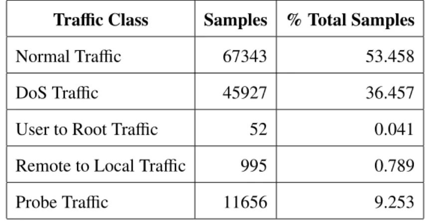
3.4.1 NSL-KDD Evaluation Workload Creation. This research uses a subset of the NSL-KDD train+.txt file for its evaluation and performs k-fold cross-validation to
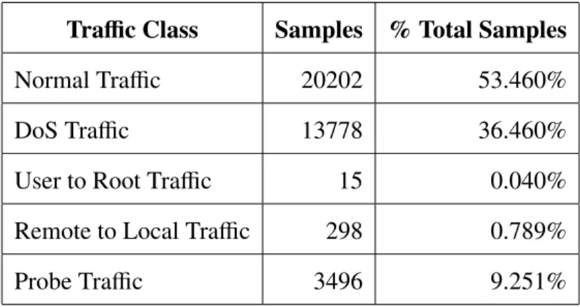
evaluate the performance of the classifiers [TBL09b][RuN09]. The dataset is split into ten folds. The classifier is trained on nine folds and tested on the last fold. This is repeated ten times using each fold as a test set and the results are collected. The train+.txt file contains 125,973 training examples with the class distribution shown in Table 3.1.