Hydrologic Evaluation of Surface and Subsurface Water in Highly Managed Watershed with Limited Observations

(1)

Clemson University

TigerPrints

All Dissertations Dissertations

8-2018

Hydrologic Evaluation of Surface and Subsurface

Water in Highly Managed Watershed with Limited

Observations

Aws Abdulqader Ajaaj

Clemson University, [email protected]

Follow this and additional works at:https://tigerprints.clemson.edu/all_dissertations

This Dissertation is brought to you for free and open access by the Dissertations at TigerPrints. It has been accepted for inclusion in All Dissertations by an authorized administrator of TigerPrints. For more information, please [email protected].

Recommended Citation

Ajaaj, Aws Abdulqader, "Hydrologic Evaluation of Surface and Subsurface Water in Highly Managed Watershed with Limited

Observations" (2018).All Dissertations. 2233.

(2)

Hydrologic Evaluation of Surface and

Subsurface Water in Highly Managed

Watershed with Limited Observations

A Dissertation Presented to the Graduate School of

Clemson University

In Partial Fulfillment

of the Requirements for the Degree Doctor of Philosophy

Civil Engineering

by

Aws Abdulqader Ajaaj August 2018

Accepted by:

Dr. Ashok. K. Mishra, Committee Chair Dr. Abdul A. Khan, Committee Co-Chair

Dr. N. Ravichandran Dr. Charles Privette, III

(3)

Abstract

The risk associated with managing water resources (flood or drought) de-pends on the adequate operation of infrastructure facilities (e.g., dams) with in the river basins. However, one of the major challenges to develop and operate infras-tructures to meet stakeholder’s goal is to generate accurate hydrologic information (e.g., streamflow) for ungagged (limited data/data scarce) river basins. This process usually requires spatiotemporal hydroclimatic information, such as precipitations, streamflow, and groundwater storage. Hydrological models are useful tools for inves-tigating hydrological processes in data scarce river basins with limited hydrological measurements. The overall objective of this dissertation is to develop a modeling framework to improve surface and groundwater resources management in data scarce river basins, located in different parts of the world.

This dissertation examines the improvements of the estimations, simulation, and evaluation of various spatiotemporal hydroclimate data for a river basin located in a semi-arid climate zone and poorly represented by actual observations. First, a modeling framework is developed and applied to investigate multiple bias removal techniques to improve the use of available gridded precipitation products in poorly gauged river basins; secondly, the study is extended to investigate hydrologic processes and to simulate streamflow for ungagged river basins using different precipitation data sources; and finally an integrated surface and groundwater modeling framework

(4)

was developed to evaluate potential surface and groundwater resources in Tigris and Euphrates River Basin.

(5)

Dedication

This work is dedicated for my beloved mother and father, Sadiyah Muhammad and Abdulqader Ajaaj, for their kindness, endless love, and support which will be a continues source of inspiration to me.

(6)

Acknowledgments

I would like to deeply thank my advisors, Dr. Ashok. K. Mishra and Dr. Abdul A. Khan, who have always given me support and motivation during the years of their mentorship for me as a PhD student. It was a privilege to work under their supervision and I will never forget this learning experience during all this time.

I would also like to thank Dr. N. Ravichandran and Dr. Charles Privette, III for accepting to serve in my committee. I am thankful for them their support, guidance, and providing valuable insights which helped improving my Dissertation.

I would like to acknowledge of my parents, brothers, and sisters for the con-tinues encouragement during hardships. I would like to thank my wife, Hind A. Ali, and my children who have giving me support, love, and ease during this journey of pursuing my dream in getting the PhD degree. Especially, my wife was the one who took care of me and our children during my busy days. I could not accomplish this without her being beside me.

I also want to extent my appreciation for all of my dear friends; especially Anoop, Goutham, and Ali for their help in clearing out many issues about the data and giving suggestions that made the research better. Finally, I am grateful to the staff members of Glenn Department of Civil Engineering for the welcoming atmo-sphere and the extended help with any type of administrative service they provided.

(7)

List of Tables

2.1 Geographic information and climate type for the selected cities. . . . 15 2.2 Percentage of urban/peri-urban areas registered significant trend (at

5% significance level) using MK1, MK2, and MK3 tests. . . 20 2.3 Trend analysis of air temperature using MK1/MK2/MK3 tests for

ur-ban and corresponding peri-urur-ban areas. Significant trends tested at 95% confidence level (i.e. |Z|>1.96 ), are shown as bold letters. . . . 24 2.4 Decadal slope obtained from linear regression for air temperature

dur-ing the period 1901-2008. . . 28 2.5 Trend analysis of precipitation using MK1/MK2/MK3 tests for urban

and corresponding peri-urban areas. Significant trends are considered at 95% confidence level (i.e. |Z| ), are shown as bold letters. . . 30 2.6 Decadal slope for precipitation based on linear regression line during

the period 1901-2010. . . 32 3.1 Bias correction techniques commonly used in hydro-climatic studies. . 47 3.2 Information for all the rainfall stations in the Iraq area. . . 56 3.3 Performance Index (PI) of individual BCT. . . 63 4.1 Streamflow gauging stations located in Tigris River Basin and used in

this study. . . 85 4.2 List of parameters and their default ranges used for the SWAT model

development. . . 89 4.3 Rank of most sensitive model parameters resulted from sensitivity

anal-ysis for four precipitation products. . . 90 4.4 Quantitative Statistics (CC, RMSE, and PBIAS) for area-averaged

daily mean annual cycle precipitation from PDS and APD in Tigris River Basin. . . 95 4.5 Correlation metrics based on CC, NS, and PBIAS calculated based

on observed streamflow and SWAT based flows obtained from differ-ent precipitation data sources. Each cell has two values represdiffer-enting calibration/validation respectively. . . 100 5.1 Previous studies that investigated coupled SWAT-MODFLOW models

(10)

5.3 Streamflow gauging stations located in TERB and used in this study. 130 5.4 An overview of data used in this study . . . 131 5.5 The ∆TWS components represented in SWAT-MODFLOW water

bal-ance equation . . . 134 5.6 Final Calibrated model parameters used for TERB modeling; these

pa-rameters were obtained from available data and adjusted during model calibration. Parameters are divided in the five subcategories based on their geographical regions in the SWAT-MODFLOW model. . . 138 5.7 Mean monthly water budgets averaged for all sub-basins in the TERB

(11)

List of Figures

2.1 Location of selected mega cities and their urban and peri-urban bound-aries. The blue polygon represents the urban area selected based on the surface imperviousness. The green polygons represent the peri-urban areas. . . 17 2.2 Percentage of imperviousness for the selected urban areas. . . 19 2.3 Variations of mean monthly precipitation for the selected cities

calcu-lated from GPCC data for the period 1901-2010. . . 22 2.4 Box plot of mean slopes based on decadal change in air temperature

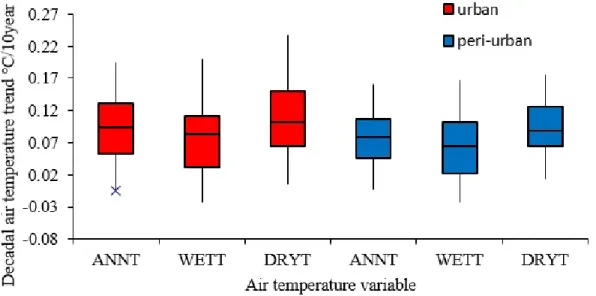
during the period 1901-2008. [Steps used: (a) for a selected city, the time series is divided into decades, (b) the slopes associated for each decade are calculated, (c) the mean of decadal slope is calculated for each city, and (d) the box plot is constructed based on the mean of decadal slope calculated for the 18 selected cities] . . . 26 2.5 Linear trends based on 5-year moving average of annual air

tempera-ture for urban and peri-urban areas . . . 29 2.6 Box plot of mean slopes based on decadal change in precipitation.

[Steps used: similar to Figure 2.4]. . . 31 2.7 The linear trends based on 5-year moving average for annual

precipi-tation for the period 1901-2008 for urban and peri-urban areas. . . . 34 2.8 Spatial distribution of Z statistics based on MK3 test for annual

pre-cipitation (1901-2010) in urban and peri-urban areas. . . 35 2.9 Spatial distribution of Z statistics based on MK3 test for wet season

precipitation (1901-2010) in urban and peri-urban areas. . . 36 2.10 Spatial distribution of Z statistics based on MK3 test for dry season

precipitation (1901-2010) in urban and peri-urban area. . . 37 2.11 Scatter plot between mean decadal slopes based on annual air

temper-ature and precipitation for urban and peri-urban areas. . . 38 2.12 Scatter plot between: (a) mean decadal slope of annual, wet and dry

seasons air temperature and the percentage of imperviousness for ur-ban areas, (b) mean decadal slope of annual, wet and dry seasons precipitation and the percentage of imperviousness for urban areas. . 40

(12)

3.1 The location of climate zones and rain-gauge stations in Iraq. Red solid lines denote the boundaries of the five zones NEMZ, NVZ, WZ, CFZ, and SDZ referred as mountains area in northeast, hills area in north, west area, Central area, and southwestern area, respectively. Rainfall stations are shown in Table 3.2. . . 55 3.2 Box plots of average precipitation in Iraq for different temporal bands

from 1935 to 1958. (a) winter, (b) spring, (c) summer, (d) fall, (e) annual [Note: The x-axis represents time interval, y-axis represents mean annual or seasonal rainfall amount in millimeters]. . . 58 3.3 Variation of observed average annual precipitation from 1935 to 1958

over different zones of Iraq. Solid black lines represent different to-pographical terrains: NEMZ, NVZ, WZ, CFZ, and SDZ namely as mountains area in northeast, hills area in north, Western Plateau, Al-luvial plain, and desert area, respectively. . . 60 3.4 Spatial distribution of bias calculated based on the average annual

and seasonal monthly observed and GPCC rainfall data for 24 years (1935−1958) over Iraq: a) annual, b winter (January, February, and December), c) spring (March, April, and May), and d) fall (October, and November). The small green dots identify the stations locations. 62 3.5 Distribution of Bias correction techniques (BCT’s) for during winter

months: a) January, b) February, and c) December. . . 65 3.6 Time series showing gauge, GPCC and bias corrected data for MSL

station for the month of January (1935-1958). . . 66 3.7 Time series showing gauge, GPCC and bias corrected data for KUT

station for the month of January (1935−1958). . . 68 3.8 Distribution of Bias correction techniques (BCTs) for GPCC data

dur-ing sprdur-ing months: a) March, b) April, and c) May. . . 69 3.9 Distribution of Bias correction techniques (BCT’s) for GPCC data

during months of: a) October, b) November. . . 70 3.10 Distribution of Bias correction techniques (BCT’s) for GPCC data

during, a) Wet Season, and b) Average season. . . 72 3.11 Time series showing gauge, GPCC and bias corrected data for MSL

station for the month of January (1980-2004). . . 73 3.12 Goodness of fit test results for the bias corrected monthly and seasonal

GPCC precipitation for the period (1980−2004). Columns indicate the percentage of BCTs performed well based on: a) correlation coefficient (R), b) standard deviation ratio (RSR) test, and c) Willmott index of agreement (d). . . 74 4.1 Tigris River Basin location map: (a) DEM with stream gauges, (b)

(13)

4.2 (a) Mean monthly precipitation over Tigris River Basin based on APD (1957-1963); APHRODITE, MSWEAP, and CPC (1979-1997); and PERSIANN-CDR (1983-1997), (b) Empirical cumulative probability function (ECDF) for monthly precipitation data. . . 93 4.3 Long-term mean annual precipitation for Tigris River Basin derived

from (a) APD, (b) APHRODITE, (c) MSWEP, (d) CPC, and (e) PERSIANN-CDR data. . . 94 4.4 Calibrated model parameter range (black rectangles) and best-fit

pa-rameter values (green lines) for SWAT model derived based on five precipitation products. M DLAP D is calibrated using GRPS while

the other four models are calibrated based on CRPS approaches. ∆ represents the range of parameters. [Note: The five sets of precip-itation products are used as inputs to SWAT and the corresponding modeled streamflow outputs are represented byM DLAP H,M DLM SW, M DLCP C, M DLP ER, and M DLAP D]. . . 98

4.5 Simulated monthly streamflow for four gauging stations estimated from SWAT model with different PDS. TIGBSN4 and TIGBSN7 stations are located on the main Tigris River, while TIGBSN1 and TIGBSN6 stations are located on its tributaries. . . 102 4.6 p- and r-factors from SWAT models (shown as groups) calibrated with

CRPS, GRPS, and IRPS methods. Each group represents a model calibrated using three approaches. Three pairs of boxes in each group are presented with the first box being for calibration and the second box for validation in each pair. . . 104 4.7 Illustration of 95PPU intervals obtained from SUFI-2 for CRPS and

IRPS approaches. Model results are presented for TIGBSN2 stream-flow station. The left side panel represents simulation results for CRPS calibration approach, while the right column is simulation results ob-tained based on IRPS approach. Rows are arranged as follows (a) APHRODITE, (b) CPC, (c) MSWEP, and (d) PERSIANN-CDR. . . 106 4.8 Illustration of 95% uncertainty intervals obtained from SUFI-2 for

CRPS and IRPS approaches. Models result are presented for TIG-BSN3 streamflow station. The left side column represents simulation results for CRPS approach, while the right column is simulation results obtained based on IRPS approach. Rows are arranged as follows (a) represents APHRODITE, (b) CPC, (c) MSWEP, and (d) PERSIANN-CDR. . . 107 5.1 Location and general features of the Tigris and Euphrates river basin,

Middle East. . . 118 5.2 Coupled SWAT-MODFLOW watershed hydrologic modeling

(14)

5.3 Long-term mean monthly precipitation over the study area for the period (1951-2007). The data sets are based on APHRODITE precip-itation data for Asia. . . 126 5.4 Surficial geological layers of the TERB and vertical stratigraphy for

the study area. . . 128 5.5 Relationship between simulated and observed mean monthly well

ground-water levels in the TERB. . . 136 5.6 Basin mean of total water storage anomalies for the TERB (a)

Cor-relation between mean annual TWS obtained from SWAT-MODFLOW and GRACE data. (b) Annual TWS obtained from SWAT-MODFLOW and GRACE data for the period 2003-2013. . . 139 5.7 Long-term mean annual groundwater recharge (mm) for the TERB

obtained from SWAT model for the period 1981-1997. . . 142 5.8 Hydrographs for selected stream gauge stations simulated from fully

coupled SWAT-MODFLOW output showing the observed, the best simulation, and the 95% prediction uncertainty (95PPU) streamflow. At each station about two-third of the data was used for calibration and the remaining for validation. . . 144 5.9 Long-term mean annual groundwater discharges (m3_y−1_{) for the TERB}

obtained from SWAT-MODFLOW model for the period 1981-1997. . 145 5.10 Monthly discharges between groundwater and streams (m3/month)

ex-pressed as, (a) average of long-term mean monthly (b) mean monthly for the TERB in the period 1979-1997. . . 146 5.11 Long-term mean water table elevation for the entire study area

(15)

Chapter 1

Introduction

1.1

Overview

Urban areas have traditionally developed near rivers and flood plains where the water management is directly linked to community development. With that, risks associated with floods and droughts have become critical and need to be considered for public policy and infrastructure planning. One such example is the water management issues in the Mesopotamia, the largest river system in the Middle East, which has been of a long struggle between the riparian countries, Turkey, Iran, Iraq, and Syria (Jaradat, 2002). Aggressive water management policies have been implemented by countries located in the upstreams to meet the increasing irrigation and population water demands (Altinbilek 2004; Bozkurt and Sen, 2013). The effect of water stress is further compounded by the declining mean annual streamflow. For example, flow observed at Kut station, southern part of the river basin, was reduced by about 50 m3s−1 from 1931-1973 to 1974-2004, given similarity in mean annual precipitation in these two periods (473.34 mm and 472.80 mm, respectively) (Ajaaj et al., 2017). Thus, it can be suggested that the areas located in the downstream of the watershed

(16)

are vulnerable to extreme drought under such management plans (Wilson, 2012; Issa et al. 2015).

Given that more people in the southern areas of Mesopotamia (approximately 75%) rely on the ground water, the region has witnessed a loss of large parts of their water storage due to the extensive pumping of the groundwater from the aquifer systems with the lack of precipitation (drier arid areas; Ajaaj et al., 2017). Under such conditions, several studies raised the concerns of severe negative consequences on health, environment, and the ecosystem due to change in water quality and quantity in the freshwater with in the river basin (Altinbilek D., 2004; Al-Ansari and Knutsson, 2011). Currently,there have been severed challenges in the river basin. For instance, low surface flow and groundwater depletion and reduction in water storage and quality (Issa et al. 2015; Wilson, 2012; Venn et al. 2013; Voss et al., 2013); degradation of agricultural lands (Jabbar and Zhou, 2012) and drying of wetlands and marshlands (Jones et al., 2008) southern parts of TERB; alteration of waterways due to low flow caused by rivers damming (Nilsson et al., 2005); and increasing salinization in agricultural lands (Wu et al., 2012).

1.2

Limitations with Observed Hydroclimate Data

The assessment of regional water resource availability for any river basin is quantified by the spatial distributions of hydrologic fluxes, such as rainfall, stream-flow, and groundwater variations (Kundzewicz et al. 2007). One major challenge for improving water resources management is lack of long term hydroclimatic infor-mation. This is evident due to a marked decline in hydroclimatic gauging stations in many parts of the world during past decades (Song et al. 2014; Rodda 1995a, b; Mishra and Coulibaly 2009). Due to the lack of long term hydroclimatic information,

(17)

water resources managers find it difficult to generate historical (i.e., beyond 50 years) water availability and drought information in many parts of Africa, Latin America, and Asia (WMO 1996; Mishra and Coulibaly 2009).

Another factor that affects water management is human activities and chang-ing land cover in urban areas which play an important role in alterchang-ing local to regional climate. Currently, more than 50% of the global population lives in cities, and it is projected to be 70% by 2050 (UNFPA 2007). The expansion of global urban area was about 60,000 km2 during 19702000 (Seto et al. 2011) and it is projected to in-crease by 1.7 million km2 _{in the less-developed countries during 2000 to 2050 (Angel}

et al. 2011). Development of urban areas significantly alters the natural land cover. Consequently, it has been suggested that human activities in cities lead to a dis-tinct urban climate (e.g., urban heat island) in comparison to the less built-up areas. These changes are primarily attributed to three drivers including land cover change, greenhouse gas, and aerosols (Niyogi et al. 2009; Rosenzweig et al. 2011; Liuet al. 2014). The climate change can bring additional stresses to the urban environment leading to heat waves, extreme urban flood, and health problems for vulnerable urban populations (Rosenzweig et al. 2011).

1.3

Applications of Remote Sensed Precipitation

in Hydrological Modeling

With the advancements in satellite rainfall products, it is now possible to ap-ply/evaluate these products to investigate hydrological processes in poorly gauged basins. Hydrological models are useful tools for evaluating the water resources in watersheds with limited hydrological measurements (Amisigo et al, 2008; Hongxia et

(18)

al, 2009; Abbaspour et al, 2015). The precipitation data is considered as one of the most important driving forces for hydrologic models (Beven, 2011; Miao et al., 2015). Moreover, the long-term rainfall data are important for developing metrics (i.e., risk, uncertainty and vulnerability) to evaluate climate change impact assessment by com-paring past extreme events.

Several remote sensing (satellite-based) precipitation products have been re-cently evaluated (validated) against in-situ precipitation for streamflow simulation us-ing hydrological models (Behrangi et al., 2011; Ali et al., 2017). The ongous-ing efforts for improving remotely sensed measurements have produced many high-resolution (<4 km) and temporal (<3 hours) precipitation products (Sorooshian et al., 2000). Recently there are several studies evaluated the performance of satellite-based pre-cipitation products to predict streamflow in data sparse regions using hydrological models. For example, Thiemig et al., (2013) and Zhu et al., (2016) evaluated the use of satellite precipitation data in the hydrological applications and reported that two satellite-based precipitation products named TRMM and PERSIANN-CDR per-formed better in comparison to the reanalysis gauged-based data. Many studies have concluded that satellite-based precipitation products could be potentially used for hydrological predictions particularly for ungauged basins (Xue et al., 2013; Jiang et al., 2012).

However, the uncertainty associated with hydrological models, especially when using different model inputs greatly affects the model performance. This may lead to less meaningful and sometimes misleading predictions if such uncertainties are not addressed in the calibration process (Vrugt and Bouten, 2002; Schuol and Abbaspour, 2006; Yang et al., 2007 a, and b). In model calibration, instead of relying on a single model prediction, statistical methods are used to represent uncertainties in hydrolog-ical models, where such uncertainties are given a probabilistic range to account for

(19)

several sources of errors in the model (Franz et al. 2010).

1.4

Overall Research objectives

The overarching goal of this thesis is to improve water resources assessments in poorly gauged river basins around the world. To demonstrate our proposed meth-ods, we selected Tigris River basin as a case study. Although several studies have evaluated water resource in different parts of the world (Mishra and Coulibaly, 2010; Taesombat and Sriwongsitanon, 2009; Jones et al., 2008), the studies on investigating the combined role of climatic variables, anthropogenic control (e.g., land use change) in an integrated surface and ground water modeling framework is limited. A detailed literature review is available for each research objectives proposed in this thesis. The overall four research objectives are proposed in this thesis:

First objective-Trends in precipitation and air temperature:- To investigates

the trends in annual and seasonal monthly precipitation and temperature of mega cities around the globe by applying multiple trend analysis methods. This objective evaluates trends in long-term climatologies by incorporating land use change in urban verses peri-urban areas for mega cities located in various cli-mate zones.

Objective 1.1: To investigate annual and seasonal trends in precipitation and air temperature for urban/peri-urban areas of mega cities.

Objective 1.2: To quantify the decadal change in air temperature and

precipitation as well as their possible relationship.

(20)

pro-to improve the use of available gridded precipitation products in poorly gauged river basins.

Objective 2.1: To test multiple BCT’s on monthly precipitation data to

select the best method that fits each gauge station in semi-arid climate.

Third objective-Hydrologic evaluation of precipitation data sources:- The study

is extended to investigate hydrologic processes and to simulate streamflow for Tigris River Basin, un-gagged river basin, from different precipitation data sources.

Objective 3.1: To evaluate the spatiotemporal heterogeneities of multiple precipitation data sources against actual gauged data.

Objective 3.2: To evaluate the suitability of using precipitation data sources to simulate streamflow in Tigris River Basin given limited hydroclimate in-formation.

Objective 3.2: To investigate the predictive uncertainty in simulating stream-flow using three calibration approaches to improve streamstream-flow simulation.

Fourth objective-Surface and groundwater resources assessment:- River basins

in semi-arid climates are likely to be vulnerable to extreme water stress condi-tions under projected climate change scenarios (Huetal.2016; Sun et al. 2014; Di Luca et al. 2015). Therefore, we developed an integrated surface and groundwa-ter modeling framework to investigate wagroundwa-ter resources in Tigris and Euphrates River Basin.

Objective 4.1: To apply the fully coupled SWAT-MODFLOW model to

(21)

the river basin.

Objective 4.2: To test model outputs against streamflow, groundwater lev-els, and total water storage anomalies derived from satellite data (GRACE) especially with the lack of actual observations.

Objective 4.3: To predict the discharges that exchange between streams

and groundwater in aquifers. Also, to estimate the spatial and temporal variations of infiltration and evaporation losses from different surfaces in the watershed.

1.5

Thesis Organization

This thesis contains six chapters with the main body of research presented in

Chapter 2 to Chapter 5. The following research points are presented into four

journal papers with two already published papers (Ajaaj et al., 2016; Ajaaj et al., 2017).

Chapter 2presents a conservative approach in detecting trends of long term

precipitation and temperature (>100years) using different trend analysis approaches. This chapter also investigates the effect of land use on the trends by considering the largest urban vs peri-urban areas in the world. This paper is published in journal of Theoretical and Applied Climatology.

Chapter 3evaluates and compares different bias correction techniques (BCT’s)

using gridded precipitation data with respect to rain gauges in semi-arid climatic zone. This work is published in Stochastic Environmental Research and Risk

Assessment.

(22)

satel-streamflow were evaluated using stochastic model approach. Additionally, the pre-dictive uncertainty in simulating streamflow using three calibration approaches was compared to improve streamflow simulation. This Manuscript is completed and was submitted to the Journal of Hydrologic Engineering.

For Chapter 5, the hydrologic model built in Chapter 4 was extended in

area and included not only the surface water component but also the groundwater modeled using three dimensional groundwater fully coupled model. In this chapter, the calibrated mode was utilized to understand the role of surface and groundwater in-teractions in the Euphrates and Tigris River Basin was investigated. This Manuscript is completed and will be send to a journal.

The section, table and figure numbers have been changed in this dissertation but all contents were kept without change. Copies of Chapter 2 and Chapter 3, papers, are provided in the Appendices A and B.

Finally conclusions, recommendation, and suggested future work are listed in

(23)

Chapter 2

Urban and peri-urban precipitation

and air temperature trends in

mega cities of the world using

multiple trend analysis methods

2.1

Abstract

Urbanization plays an important role in altering local to regional climate.In this study, the trends in precipitation and the air temperature were investigated for urban and peri-urban areas of 18 mega cities selected from six continents (represent-ing a wide range of climatic patterns). Multiple statistical tests were used to examine long-term trends in annual and seasonal precipitation and air temperature for the selected cites.The urban and peri-urban are as were classified based on the percent-age of land imperviousness. Through this study, it was evident that removal of the lag-k serial correlation caused a reduction of approximately 20 to 30% in significant

(24)

trend observability for temperature and precipitation data. This observation suggests that appropriate trend analysis methodology for climate studies is necessary. Addi-tionally, about70% of the urban areas showed higher positive air temperature trends, compared with peri-urban areas. There were not clear trend signatures (i.e., mix of increase or decrease) when comparing urban vs peri-urban precipitation in each selected city. Overall, cities located in dry areas, for example, in Africa, southern parts of North America, and Eastern Asia, showed a decrease in annual and seasonal precipitation, while wetter conditions were favorable for cities located in wet regions such as, southeastern South America, eastern North America, and northern Europe. A positive relationship was observed between decadal trends of annual/seasonal air temperature and precipitation for all urban and peri-urban areas, with a higher rate being observed for urban areas.

2.2

Introduction

More than 50%of the global population lives in cities, and it is projected to be 70% by 2050 (UNFPA 2007). The expansion of global urban area was about 60,000 km2 _{during 1970-2000 (Seto et al., 2011) and it is projected to increase by 1.7 million}

km2 in the less-developed countries during 2000 to 2050 (Angel et al., 2011). Devel-opment of urban areas significantly alters the natural land cover. Consequently, it has been suggested that human activities in cities lead to a distinct urban climate (e.g., urban heat island) in comparison to the less built up areas. These changes are primarily attributed to three drivers including land cover change, greenhouse gas, and aerosols (Niyogi et al., 2009; Rosenzweig et al., 2011; Liu et al., 2014). The climate change can bring additional stresses to the urban environment leading to heat waves, extreme urban flood, and health problems for vulnerable urban populations

(25)

(Rosen-zweig et al., 2011).

Several studies indicated the possible influence of global warming on intensi-fication of precipitation near urban centers (Diem and Mote, 2005; Kug and Ahn, 2013; Sun et al., 2014; Shahid et al., 2016; Han et al., 2015). A positive correlation between precipitation and urbanization has been confirmed using different climate models (Changnon and Westcott, 2002; Arg¨ueso et al., 2016). Such response in ur-ban rainfall patterns were mainly attributed to Urur-ban Heat Island (UHI; (Dixon and Mote, 2003; Bentley et al., 2010). However, there are few studies that did not agree with this hypothesis. For example, (Tayanc and Toros, 1997; Shepherd, 2006) and (Kusaka et al., 2014) found that air temperature in mega cities has no effect on urban rainfall, while (Kaufmann et al., 2007) showed a decreasing precipitation trends over urban zones. A consensus whether the urbanization results in an increase in precipitation are yet to be confirmed (Rosenzweig et al., 2011). It is often a challenge to quantify the possible impact of UHI on urban rainfall, which is further compounded by lack of accurate observed data in the vicinity of urban areas.

Climatological trends in air temperature and precipitation have been exten-sively analyzed for different regions around the world (Keggenhoff et al., 2014; Pingale et al., 2014; Sharma et al., 2016). For example, investigated the possible urban effect on precipitation over western Maritime by examining two scenarios (before and after construction of urban areas). Several studies analyzed short-term trends in sub-daily air temperature and precipitation over multi-urban areas based on the direction of predominant storms (Shepherd et al., 2002; Kharol et al., 2013; Velpuri and Senay, 2013). (Alexander et al., 2006) investigated long-term (1901 to 2003) global daily air temperature and precipitation over the Northern Hemisphere mid-latitudes (and part of Australia) and observed a significant warming and wetting trends during the

(26)

Precipitation in urban area is highly influenced by many factors such as, hy-droscopic nuclei, turbulence via surface roughness, and convergent wind flow which may lead to rain producing clouds (Burian and Shepherd, 2005). The land use change (urbanization/imperviousness) can possibly influence the urban climate due to the changes in surface albedo, surface roughness, and thermal and hydrological features (Hu and Jia, 2010). Therefore, evaluation of climatological trends in urban areas is important to plan, manage, and take actions regarding water related issues, such as water supply, avoiding over or under designing of water resource systems, and assessing the urban floods and droughts. Moreover, air temperature and precipitation trends in both urban and peri-urban areas should be examined to determine possible changes in local climatology.

2.3

Objectives

In this study, we used a long-term (>100-year period) gridded mean monthly air temperature and precipitation data to investigate: (a) annual and seasonal pre-cipitation (air temperature) trends in 18 mega cities using multiple trend analysis methods. We have selected top three mega cities from each continent and each city was further classified into urban and peri-urban areas according to their percentage of land cover imperviousness; and (b) the decadal change in air temperature and precipitation as well as their possible relationship.

2.4

Study area

Three densely populated urban areas (>5 million people in population) from each of the six continents; namely, Asia (AS), North America (NA), Africa (AF),

(27)

South America (SA), Europe (EU), and Australia (AU) were selected based on the population data provided by Environmental Systems Research Institute (ESRI). The geographic and climate information for the selected cities are provided in Table 2.1. These cities witness a wide range of climatic patterns, such as, tropical monsoon, hu-mid continental, Mediterranean, high-land climate, huhu-mid sub-tropical, huhu-mid conti-nental, oceanic climate, and semi-arid type.

The urban/peri-urban area is classified based on the percentage of the land imperviousness, (Lu and Weng, 2006). Based on this criterion, areas with impervi-ousness greater than or equal to 20% are identified as urban areas (Ganeshan et al., 2013). For each urban area, the corresponding peri-urban area was delineated using a band width of 80.5 km (50 miles) from urban boundaries. The delineation between urban and peri-urban areas was accomplished manually using the Geographic Infor-mation System (GIS) maps. The band width of the peri-urban area was selected to include at least one precipitation and air temperature grid point within the selected polygon. Selected urban and their corresponding peri-urban areas are shown in Fig-ure 2.1. The percentages of imperviousness (land use) for the selected cities are shown in Figure 2.2, where the percentages refer to the land imperviousness.

2.5

Data

Long-term Terrestrial Air Temperature (TAT) monthly data available for the period 1900-2008 was used in this study. TAT data is compiled from actual station data gathered from several updated sources (e.g., Global Historical Climatology Net-work GHCN2) with support from the Institute of Global Environmental Strategies (IGES).

(28)

version 7) precipitation data (Schneider et al., 2014), are used to compare the pre-cipitation trends in urban (peri-urban) areas. One of the main reasons for selecting GPCC data was the availability of long-term data sets for 110-year period (1901-2010). The GPCC data is derived from rain gauge information (over 85,000 stations worldwide) acquired from multiple sources and updated continuously to generate re-analysis product. GPCC compared well with observed data, for example, (Funk et al., 2015) reported that interpolated data from GPCC reanalysis version 6 precipitation product performed well when compared with station data in Africa even though the lack of actual station data.

Both TAT and GPCC data were reviewed for missing data. Grid points with one or more year of missing data were removed from the analysis. The missing data for shorter duration was estimated by taking the mean of the four surrounding grid points. The newly developed 1 km resolution Global Land Cover-SHARE (GLC-SHARE) shape file created by Food and Agriculture Organization (FAO) (Latham et al., 2014) was used to distinguish grids located within urban and peri-urban boundaries.

2.6

Methodology

This section describes four different methods used to for trend analysis for air temperature and precipitation over selected cities.

2.6.1

Linear least square fit (LR)

The linear least square fit is given by Eq.(2.1) and Eq.(2.2). Wheret is sample number (t=1, 2, ...,n; n being the length of the sample), Z(t) is the variable being considered (such as air temperature or precipitation), and indicate average values

(29)

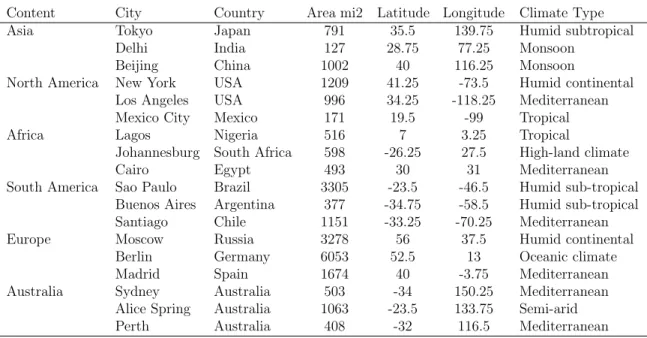
Table 2.1: Geographic information and climate type for the selected cities. Content City Country Area mi2 Latitude Longitude Climate Type Asia Tokyo Japan 791 35.5 139.75 Humid subtropical

Delhi India 127 28.75 77.25 Monsoon Beijing China 1002 40 116.25 Monsoon

North America New York USA 1209 41.25 -73.5 Humid continental Los Angeles USA 996 34.25 -118.25 Mediterranean Mexico City Mexico 171 19.5 -99 Tropical Africa Lagos Nigeria 516 7 3.25 Tropical

Johannesburg South Africa 598 -26.25 27.5 High-land climate Cairo Egypt 493 30 31 Mediterranean South America Sao Paulo Brazil 3305 -23.5 -46.5 Humid sub-tropical

Buenos Aires Argentina 377 -34.75 -58.5 Humid sub-tropical Santiago Chile 1151 -33.25 -70.25 Mediterranean Europe Moscow Russia 3278 56 37.5 Humid continental

Berlin Germany 6053 52.5 13 Oceanic climate Madrid Spain 1674 40 -3.75 Mediterranean Australia Sydney Australia 503 -34 150.25 Mediterranean

Alice Spring Australia 1063 -23.5 133.75 Semi-arid Perth Australia 408 -32 116.5 Mediterranean

(Haan, 2002). b = Pn i=1(t−¯t)(Z(t)−Z¯) Pn t=1(t−¯t)2 (2.1) a= ¯Z−b¯t (2.2)

2.6.2

Mann-Kendall test (MK1)

The Mann−Kendall (MK) nonparametric test was first proposed by (Mann, 1945) and then (Kendall, 1975). The MannKendall test statistic S is given by Eq.(2.3) and variance of S is given by Eq.(2.5). The standardized normal test statistics is computed using Eq.(2.6);

S = n−1 X k=1 n X j=k+1 sign(xj−xk) (2.3)

(30)

sign(xj −xk) =                1, for sign(xj −xk)> 0 0, for sign(xj −xk) = 0 −1, for sign(xj −xk)< 0 (2.4) V(S) = n(n−1)(2n+ 5) 18 (2.5) Z =                S−1 √ V(S), if S > 0 0, if S = 0 S+1 √ V(S), if S < 0 (2.6)

A positive (negative) value of Z indicates upward (downward) trend in the time series being tested (Luo et al., 2008); (Dr´apela et al., 2011). The advantage of MK1 is that it is distribution free test and insensitive to the outliers. However, the MK1 test requires the data to be serially uncorrelated or in other words the time series data should be independent (Yue et al., 2002); (Kumar et al., 2009). The MK test is widely used for trend analysis in hydro-climatic variables (Mishra et al., 2011); (Mishra and Singh, 2010).

2.6.3

Mann-Kendall test with trend-free pre-whitening (MK2)

The trend free pre-whiting process (TFPW) was proposed by (Yue et al., 2002) as a way to remove the serial correlation from the data before applying MK1 test. De-trending the time series is a necessary step to remove the effect of a significant linear trend on the serial correlation. It is demonstrated in Eq.(2.7), whereX_t0 is the de-trended data, Xt is the original data, slope (b) is calculated using the Theil-Sen

(31)

Figure 2.1: Location of selected mega cities and their urban and peri-urban bound-aries. The blue polygon represents the urban area selected based on the surface imperviousness. The green polygons represent the peri-urban areas.

(32)

Approach (TSA), and t is the time.

X_t0 =Xt−bt (2.7)

Then lag-1 serial correlation can be removed from de-trended time series by using Eq.(2.8). WhereY_t0a trend-free and pre-whitened time series, andr1is the lag-1

serial correlation for the de-trended time series. The residuals are added to the time series data to get the blended time series as in Eq.(2.9), which is less influenced by serial correlation. Finally, the MK1 test is applied on the final data set as described in Section 2.6.2.

Y_t0 =X_t0−r1Yt0−1 (2.8)

Yt=Yt0+bt (2.9)

2.6.4

Mann-Kendall test with variance correction (MK3)

To overcome the limitation of the presence of serial autocorrelation in time series, a correction procedure was proposed by (Hamed and Rao, 1998). First, the corrected variance S is calculated by Eq.(2.10), where V(S) is the variance of the MK1 and CF is the correction factor due to existence of serial correlation in the data. This correction factor was suggested by (Hamed and Rao, 1998) and (Yue et al., 2002) and given by Eq.(2.11), where rR

k is lag-ranked serial correlation, while n is the total number of observations.

(33)

Figure 2.2: Percentage of imperviousness for the selected urban areas. CF = 1 + 2 n(n−1)(n−2) n−1 X k=1 (n−k)(n−k−1)(n−k−2)rR_k (2.11)

The advantage of MK3 test over MK2 test is that it includes all possible serial correlations (lag-k) in the time series, while Mk2 only considers the lag-1 serial correlation (Yue et al., 2002).

(34)

2.7

Results

The selected cities are located in a wide range of climatic zones; therefore, they witness different rainfall, air temperature, and wet (dry) seasons. For example, Johannesburg winter months are counted from May to September, while in Delhi from November to January. For this reason, the year was divided into two distinct groups as wet and dry spells (or seasons). For each city, wet spell includes the months in which the total rainfall exceeds the average annual rainfall. The dry spell includes the months with total rainfall less than the average annual rainfall.The average monthly precipitation pattern for each city is presented in Figure 2.3, which clearly shows the variation of wet and dry seasons for different cities analyzed in this study. The mean of annual, dry and wet season precipitation was calculated from the GPCC monthly data for the period 1901 to 2010.

Table 2.2: Percentage of urban/peri-urban areas registered significant trend (at 5% significance level) using MK1, MK2, and MK3 tests.

Method Urban Peri -urban Urban Peri -urban ANNTa _WETT _DRYT _ANNT _WETT _DRYT _ANNPa _WETP _DRYP _ANNP _WETP _DRYP

MK1 88.9 66.7 88.9 83.3 66.7 77.8 33.3 38.9 22.2 38.9 33.3 16.7 MK2 83.3 66.7 88.9 77.8 66.7 77.8 33.3 38.9 22.2 38.9 33.3 16.7 MK3 55.6 50 50 55.6 44.4 38.9 16.7 22.2 11.1 16.7 16.7 0

a_{The terms ANNT and ANNP shown in this table and later tables are the annual}

air temperature and precipitation,WETT and WETP represent wet season air tem-perature and precipitation, and DRYT and DRYP are dry season air temtem-perature and precipitation.

2.7.1

Comparison between Mann-Kendall tests

The trend analysis was carried out using different Mann-Kendall tests (i.e., MK1, MK2, and MK3). In order to overcome the limitations due the presence of serial correlation in annual and seasonal mean air temperature and precipitation,

(35)

MK2 and MK3 methods were applied in trend analysis. MK2 eliminates the lag-1 auto correlation by using free pre-whitening (FPW), while MK3 removes the lag-k serial correlation by variance correction (VC) method. The percentage of significant trends for air temperature and precipitation based on MK1, MK2, and MK3 test are provided in Table 2.2. When using MK1 and MK2 tests, similar number of cities have significant trend in precipitation which indicates the removal of lag-1 auto-correlation that may not have much influence on the trend analysis. This pattern is also similar for air temperature during wet and dry seasons. However, MK1 test comparatively has higher number of stations for air temperature at annual scale. As reported in Table 2.2, the number of urban areas showing significant trend decreased when auto correlation correction was applied. The lower percentage of significant trends for both air temperature and precipitation was observed in case of MK3 test in comparison to MK1 and MK2 tests. Overall, the result obtained from MK3 test is more conservative in comparison to other two tests, therefore it is important to evaluate multiple MK test in trend analysis of hydro-climatic variables.

2.7.2

Trends in air temperature

The annual, wet, and dry season mean air temperature were analyzed using MK1, MK2, and MK3 tests for the period 1901-2008 to determine whether each city is experiencing cooling or warming trends (Table 2.3).The MK1, MK2, and MK3 test results were investigated for possible influence of presence of serial-1 and serial-k correlations on significant trend results for air temperature in urban and peri-urban areas. Many of the previous studies only focused on classical MK1 test for trend analysis in hydro-climatic time series, which ignores the presence of correlation in time series (Karabulut et al., 2008); (Karmeshu, 2012). However, we observed that MK3

(36)

Figure 2.3: Variations of mean monthly precipitation for the selected cities calculated from GPCC data for the period 1901-2010.

(37)

results provide a conservative estimate after removing all forms of serial correlations. Overall, there is an increasing trend for urban and peri-urban annual and seasonal air temperature. Based on the MK3 results (Table 2.3), it was observed that 70% of the urban areas experienced warmer trend (i.e., Z > 0) in annual and seasonal air temperature in comparison to the peri-urban areas. Significant warming trends are found in about 56% of urban areas (likewise for peri-urban areas) based on annual air temperature. None of the urban and peri-urban areas register a significant cooling trend based on annual and seasonal air temperature. However, the urban air temperature in wet and dry seasons illustrates higher significant trends (i.e., Z

> 1.96) than peri-urban areas. About 50% of urban areas show significant warming trends, whereas for peri-urban areas, these values are lower than those in the urban areas with about 44 and 39% during wet and dry seasons, respectively. Significant warming trends in annual air temperature are observed in Tokyo and selected cities in North America, Johannesburg, Sao Paulo and Buenos Aires, and Moscow and Madrid. Urban areas located in Australia do not show any significant trend for annual air temperature; these urban areas show the lowest imperviousness among all selected urban areas, Figure 2.2.

We applied linear regression method to estimate the magnitude of change in air temperature with respect to time. The change in annual and seasonal air tem-perature over a 10-year period for urban and peri-urban areas is shown in Figure 2.4. The rectangular box plot shows three horizontal lines that represent the median (in-termediate line), 25th _{percentile (lower line), and 75}th _{percentile values (upper line),}

while the two top and bottom vertical lines represent the maximum and minimum changes over the 10-year period for the urban and peri-urban areas. The results show that the median rise in urban annual and seasonal air temperature is higher than that

(38)

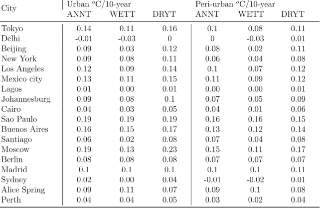
T able 2.3: T rend analysis of ai r temp erature using MK1/MK2/MK3 tests for urban and corresp onding p eri-urban areas. Significan t trends tested at 95% confidence lev el (i.e. | Z | > 1 . 96 ), are sho wn as b old letters. Cit y Urban P eri -urban ANNT WETT DR YT ANNT WETT DR YT T oky o 7.77/7.71/2.29 5.65/5.55/2.33 7.47/7.53/2.13 6.16/6.1/2.23 4.63/4.58/2.33 5.7/5.67/2.02 Delhi -0.59/-0.48/-0.67 -1.3/-1.09/-1.35 0.39/0.3/0.48 -0.33/-0.01/-0.4 -0.92/-0.68/-1 0.67/0. 58/0.91 Beijing 4.31/5.97 /1.77 2.2/3.2/1.24 5.45/5.98/2.02 3.88/5.41 /1.67 1.82/ 2.76 /1.05 5.11/5.42/2.01 New Y ork 4.32/4.16/2.22 3.48/3.57/2.14 3.48/3.24/2.12 2.6/2.33 /1.95 1 .58/1.63/1.79 2.38/2.05 /1.97 Los Angeles 6.29/6.7/2.02 6.6/6.77/2.06 4.25/4.31 /1.84 5.63/6.01/2.04 5.86/5.87/2.11 3.08/3.35 /1.72 Mexico Cit y 7.04/8.09/2.04 5.89/6.4 /1.92 7.39/7.95/2.11 6.68/7.66/2.13 6.06/6.4/2.06 6.37/7.2/2.12 Lagos -0.11/0.46/-0.06 0.33/0.9 6/0.19 -0.54/0.05/-0.25 -0.1/0.26/-0.06 0.17/0.41/0.12 -0.5/0.03/-0.29 Johannesburg 5.63/6.05/2.2 4.64/4.93/2.11 5.36/5.37/2.13 4.87/4.95/2.13 3.23/3.24 /1.87 5.08/5.11/2.07 Cairo 2.59/3.27 /1.56 3.08/3.57 /1.68 1.73/ 2.02 /1.4 2.06/2.62 /1.22 2.93/3.67 /1.53 0.52/0.75/0.4 Sao P aulo 9.17/9.1/2.28 8.91/8.8/2.26 7.86/7.76/2.24 8.66/8.53/2.24 8.38/8.28/2.22 7.14/6.99/2.2 Buenos Aires 9.19/9.25/2.25 7.12/7.05/2.17 7.61/7.95/2.15 8.06/7.96/2.23 6.16/6.05/2.2 6.35/6.85/2.08 San tiago 4.2/4.71 /1.77 5.99/6.61 /1.97 1.49/1.89/1.34 5.06/5.39/2.05 6.49/6.88/2.15 2.47/2.81 /1.81 Mosco w 5.66/5.78/2.19 5.09/5.32/2.22 4.23/4.22/1.99 4.49/4.57/2.19 4.19/4.33/2.22 3.08/3.09 /1.91 Berlin 3.14/3.27 /1.86 3.36/3.58/2.08 1.62/1.59/1.34 2.84/3.02 /1.82 3.25/3.41/2.11 1.49/1.41/1.3 Madrid 5.75/5.58/2.27 3.48/3.65 /1.96 5.28/4.99/2.04 5.67/5.9/2.12 4.16/4.41 /1.91 4.74/4.7/2 Sydney 2.02 /1.74/1.87 0.51/0.53/0.81 3.19/3.05/2.13 -0.34/-0.27/-0.59 -1.39/-1.24/-1.72 0.96/0.5 2/1.45 Alice Spring 3.86/4.38 /1.98 4.29/4.62/2.07 2.54/2.43 /1.88 4.09/4.62/2.05 4.49/4.65/2.12 2.73/2.54 /1.95 P erth 3.01/2.86 /1.67 2.62/2.54 /1.64 2.71/2.56 /1.66 2.05/1.96 /1.52 2.07/2.08 /1.7 1.44/1.35/1.15

(39)

The magnitudes of decadal slopes for urban and peri-urban areas are presented in Table 2.4. Linear trend results indicate that about an average of 20% of urban areas experienced higher mean decadal increase in annual and seasonal air temperature in comparison to peri-urban areas. During the period 1901-2008, the average increase in air temperature for all 18 urban areas observed to be 1, 0.8, and 1.1oC for annual, wet season, and dry season, respectively. Similarly, upward trends are also observed in peri-urban areas albeit with lower rates of warming. The average increase in 18 peri-urban areas observed to be remarkably less with 0.8, 0.6, and 0.9o_{C for annual,}

wet, and dry air temperature respectively for the time period 1901-2008. For the same time period, Sao Paulo (Delhi) recorded the highest (lowest) change among all urban and peri-urban areas for annual data with 2 (-0.1)oC.

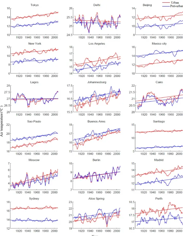
Figure 2.5 shows the linear regression and the 5-year moving average trend for the annual air temperature. It can be observed that warming signature based on urban areas is located in the Mediterranean climate except Cairo, and Monsoon climate is comparatively higher than the corresponding sub-urban areas. Further-more, the annual air temperature for peri-urban areas of Sao Paulo and Buenos Aires (both located in humid sub-tropical climate), and Johannesburg (located in high-land climate) show higher values than corresponding urban pairs. However, the rates of warming for these urban areas are relatively higher than those for the peri-urban sites Table 2.4. It can be suggested that regardless of the urban heat effect over urban areas, there is a general persistent growth of warming with time over almost all urban and peri-urban areas. For the period (1901-2008), significant warming trends were observed in mean annual and seasonal air temperature over the majority of urban and peri-urban pairs. The level of significance was found to be higher over urban areas in comparison to corresponding peri-urban areas, which indicates the clear influence of

(40)

Figure 2.4: Box plot of mean slopes based on decadal change in air temperature during the period 1901-2008. [Steps used: (a) for a selected city, the time series is divided into decades, (b) the slopes associated for each decade are calculated, (c) the mean of decadal slope is calculated for each city, and (d) the box plot is constructed based on the mean of decadal slope calculated for the 18 selected cities]

(41)

2.7.3

Trends in precipitation

Trend analysis was performed for annual and seasonal (i.e., wet and dry) pre-cipitation during the period 19012010 using MK1, MK2, and MK3 tests Table 2.5. Overall, annual and seasonal precipitation for urban and peri-urban areas shows mix (increasing and decreasing) trends unlike air temperature data. For annual precipi-tation, it was found that half of urban and peri-urban areas witness increasing trend while the other half a decreasing trend based on MK3 test. Trends in precipitation data were determined at a statistical significant level of 5% (similar to air tempera-ture analysis). A significant increase in mean annual precipitation was found in two urban and peri-urban areas while one location shows a significant decreasing trend. Significant increasing precipitation trends for annual rainfall are mainly observed in the cities of Buenos Aires and Berlin, while a significant decreasing trend was found for Cairo. Trend results of seasonal precipitation for both urban/peri-urban areas exhibit similar pattern as in annual precipitation, Table 2.5. For the wet season, only two cities (Sao Paulo and Buenos Aires) appeared to have significant increasing trends, while peri-urban areas located in Buenos Aires witness a significant increas-ing trend. Both Perth and Cairo found to have a significant decreasincreas-ing precipitation trend during wet season. For dry season, none of the urban/peri-urban areas have a positive significant trend. However, the urban areas of Cairo and Madrid show significant decreasing trend in dry season. It is worth to mention that the number of cities witnessing significant increasing (decreasing) trend is higher in MK1 and MK2 test in comparison to MK3 test, Table 2.5.

The box plot for the decadal change in precipitation was estimated using linear regression for annual and seasonal precipitation during the time period 1901-2010, Figure 2.6. The interquartile range (IQR) for decadal trends in annual and wet

(42)

Table 2.4: Decadal slope obtained from linear regression for air temperature during the period 1901-2008.

City Urban oC/10-year Peri-urban oC/10-year

ANNT WETT DRYT ANNT WETT DRYT

Tokyo 0.14 0.11 0.16 0.1 0.08 0.11 Delhi -0.01 -0.03 0 0 -0.03 0.01 Beijing 0.09 0.03 0.12 0.08 0.02 0.11 New York 0.09 0.08 0.11 0.06 0.04 0.08 Los Angeles 0.12 0.09 0.14 0.1 0.07 0.12 Mexico city 0.13 0.11 0.15 0.11 0.09 0.12 Lagos 0.01 0.00 0.01 0.00 0.00 0.01 Johannesburg 0.09 0.08 0.1 0.07 0.05 0.09 Cairo 0.04 0.03 0.05 0.04 0.01 0.06 Sao Paulo 0.19 0.19 0.19 0.16 0.16 0.15 Buenos Aires 0.16 0.15 0.17 0.13 0.12 0.14 Santiago 0.06 0.02 0.08 0.07 0.04 0.08 Moscow 0.19 0.13 0.23 0.15 0.11 0.17 Berlin 0.08 0.08 0.08 0.07 0.07 0.07 Madrid 0.1 0.1 0.1 0.1 0.1 0.11 Sydney 0.02 0.00 0.04 -0.01 -0.02 0.01 Alice Spring 0.09 0.11 0.07 0.09 0.1 0.08 Perth 0.04 0.04 0.05 0.03 0.02 0.04

(43)

Figure 2.5: Linear trends based on 5-year moving average of annual air temperature for urban and peri-urban areas

(44)

T able 2.5: T rend analysis of preci pitation using MK1/MK2/MK3 tests for urban and corresp onding p eri-urban areas. Significan t trends are conside red at 95% confidence lev el (i.e. | Z | ), are sho wn as b old letters. Cit y Urban P eri-urban ANNP WETP DR YP ANNP WETP DR YP T oky o -1.81/-1.91/-1.45 -1.49/-1.61/-1.34 -1.41/-1.36/-1.74 -1.97/-2.07/-1.69 -1.72/-1.87/-1.59 -1.44/-1.38/-1.71 Delhi 1.18/1/1.53 0.79/0.6/1.14 0.88/0.99/0.93 1.12/1/1.52 0.78/0.54/1.16 0.95/0.97 /0.99 Beijing -0.76/-0.57/-0.9 -1.22/-1.2 3/-1.15 1.9 8/1.97/1.77 -0.23/-0.09/-0.34 -0.92/-0.73/ -0.95 2.17/2.35/1.8 New Y ork 0.89/1.08/1.12 0.87/1.17/1.13 0.44/0.42/0.91 2.14/2.32/1.76 1.69/1.88/1.66 1.47/1.63/1.79 Los Angeles -0.92/-0.98/-1.38 -0.83/-0.88/-1.33 -1.09/-0.91/-1.2 -1.33/-1.37/-1.51 -1.12/-1.21/ -1.44 -1.62/-1.48/-1.49 Mexico cit y 3.3/3.25 /1.83 3.96/4.15/1.89 0. 2/-0.15/0.28 1.39/1.28/0.88 2.43/2.37 /1.35 -0.68/-0.97/-0.75 Lagos -1.61/-1.29/-1.61 -0.9/-0.73/-1.23 -2.65/-2.55/-1.54 0.08/0.31/0.13 1.04/1.26/1.23 -3.15/-3.16/-1.67 Johannesburg -1.14/-1.01/-1.8 -1.1/-1.08 /-1.55 -0.36/-0.22/-0.38 -0.51/-0.41/-0.98 -0.6/-0.49/-1 .32 -0.11/0.1 /-0.12 Cairo -3.74/-3.34/-2.09 -2.38/-2.25/-2.03 -2.11/-1.1/-2.04 -4.34/-4.35/-2.13 -3.29/-3.31/-2.14 -1.63/-0.79/-1.61 Sao P aulo 2.45/2.49 /1.74 2.91/2.71/1.98 0.46/0.44/0.7 1.98/1.99/1.63 2.46/2.33/1.83 0.4/0.48/0.62 Buenos Aires 4.64/4.51/2.08 4.81/4.74 /1.96 0.87/0.87/0.9 3 4.13/3.97/2.08 4.44/4.36/2.04 0.46/0.38/0.51 San tiago -0.94/-0.87/-1.24 -1.09/-1/-1.5 0.6/0.46/0.8 4 -0.37/-0.37/-0.52 -0.98/-0.83/ -1.19 1.87/1.67/1.87 Mosco w 4.31/4.37/1.94 2.52/2.23/1.9 4.2/4.24/1.82 4.15/4.06/1.86 2.41/2.04/1.85 4.13/4.19/1.78 Berlin 1.16/1.05/2.01 0.08/-0.06/0.17 1.27/1.3/1.59 0.95/0.89/1.98 -0.23/-0.37/-0.39 1.3/1.4/1.77 Madrid -0.58/-0.59/-0.86 0.04/0.08/0.07 -1.86/-1.97/-2.01 -0.36/-0.32/-0.52 0.2/0.13/0.3 6 -1.48/-1.43/-1.8 Sydney 1.14/1/1.14 2.3/2.05/1.5 -1.1/-1.05/-1 .6 1.2/1.12/1.07 1. 71/1.6/1.43 -0.47/-0. 51/-0.69 Alice Spring 0.75/0.75/0.95 0.36/0.47/0.6 0.15/0.01/0.25 -0.17/-0.07/-0.28 -0.33/-0.16/ -0.55 -0.4/-0.54/-0.97 P erth -2.36/-2.54/-1.9 -3.33/-3.37/-2.03 0.85/0.72/1.55 -1.96/-2.22/-1.86 -2.99/-3.13/-1.97 1.4/1.13/1.9

(45)

Figure 2.6: Box plot of mean slopes based on decadal change in precipitation. [Steps used: similar to Figure 2.4].

season precipitation for selected urban areas are comparatively higher than the peri-urban areas. This effect becomes less obvious in case of dry season. The median of decadal precipitation trends in urban areas during 1901-2010 is slightly higher than the peri-urban areas by the amount of 3.6, 1.6, and 0.5 mm/10 years for the annual, wet and dry season, respectively. An increase in mean annual and seasonal precipitation was also observed in urban averages over the surrounding peri-urban areas. The relative increase in average precipitation in urban areas with respect to peri-urban areas observed to be 41, 29.3, and 11.87 mm for annual, wet, and dry seasons, respectively, Table 2.6.

The maximum linear decadal increase for urban (and the corresponding peri-urban area) was observed for Buenos Aires with 27.87 (23.27) mm/10 years during annual precipitation, and 25.77 (22.72) mm/10 years for wet season precipitation. The lowest decadal trend in annual precipitation of urban (peri-urban) area was observed in Cairo with a value of -1.75 (-2.41) mm/10 years. The 5-year moving averages for

(46)

Table 2.6: Decadal slope for precipitation based on linear regression line during the period 1901-2010.

City Urban mm /10-year Peri-urban mm /10-year

ANNP WETP DRYP ANNP WETP DRYP

Tokyo -14.35 -11.02 -3.33 -14.3 -10.26 -4.05 Delhi 7.41 5.21 2.21 6.24 4.27 1.97 Beijing -4.14 -6.34 2.2 -0.7 -2.78 2.08 New York 4.72 2.56 2.16 9.23 4.41 4.82 Los Angeles -3.02 -2.09 -0.92 -5.4 -4.06 -1.34 Mexico City 10.96 11.55 -0.59 5.24 7.19 -1.95 Lagos -17.48 -11 -6.48 -4.32 1.93 -6.24 Johannesburg -5.72 -5.02 -0.71 -2.66 -2.34 -0.32 Cairo -1.75 -1.11 -0.63 -2.41 -1.82 -0.59 Sao Paulo 17.81 14.77 3.04 14.52 11.61 2.91 Buenos Aires 27.87 25.77 2.1 23.27 22.72 0.55 Santiago -4.99 -5.2 0.21 -1.23 -3.29 2.06 Moscow 14.69 6.43 8.26 13.22 5.57 7.65 Berlin 3.41 0.51 2.89 2.44 -0.02 2.46 Madrid -1.59 0.48 -2.07 -0.69 0.82 -1.51 Sydney 9.16 13.52 -4.36 5.85 7.17 -1.32 Alice Spring 5.59 3.75 1.84 1.71 1.36 0.35 Perth -11.29 -12.44 1.15 -5.94 -7.33 1.39

the mean annual precipitation time series are given in Figure 2.7. A general trend in annual precipitation for the urban/ peri-urban areas cannot be ascertained as both increasing and decreasing trends were observed in multiple cities. Interestingly, the significant increasing trends for both annual precipitation and air temperature were observed in urban areas of Sao Paulo and Buenos Aires (both located in humid sub-tropical climate), and Johannesburg (located in high-land climate). This obvious variation of urban precipitation signal in these locations Figure 2.5 is an option for future research direction and it deserves special attention.

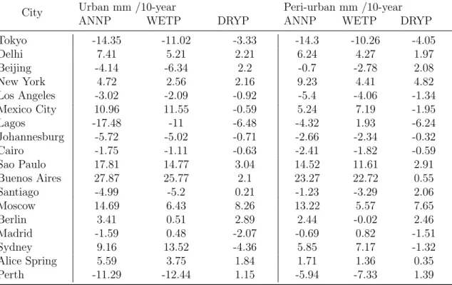
The spatial distribution of trends based on MK3 statistics for annual and seasonal precipitation data for urban and surrounding peri-urban areas was analyzed and presented in Figures 2.8, 2.9, and 2.10. It was interesting to observe difference between annual precipitation trends for some urban and peri urban areas, for example

(47)

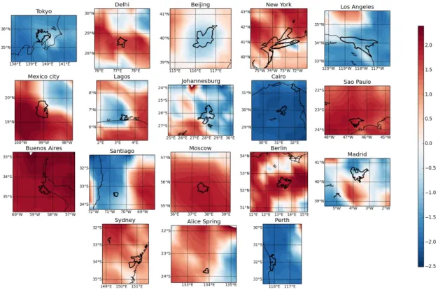
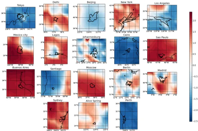
in Beijing and Lagos, where the negative trends are observed for urban whereas positive trends were observed in the vicinity of the urban polygons Figure 2.8. During the wet spell and for most locations, the negative trends in precipitation are more predominant in most urban areas Figure 2.9. Negative trends were less prevalent during the dry spells particularly in the cities of Beijing, Tokyo, and Perth. During the dry spell, positive trends are more dominated over negative trends Figure 2.10.

2.7.4

Possible Linkage between Precipitation, Temperature,

and Imperviousness

The scattered plots between decadal linear slopes of annual (seasonal) precip-itation and air temperature for selected cities are shown in Figure 2.11. A positive relationship between precipitation and air temperature was observed for all selected urban and peri-urban areas. The increments in precipitation and air temperature, however, seem to be relatively higher in urban than in peri-urban areas. This finding does not necessarily mean that higher air temperature trend results in higher precipi-tation over all urban areas because other drivers can influence the global precipiprecipi-tation such as topography and large climate oscillations.

The scatter plot between the decadal trends of annual and seasonal precipi-tation (air temperature) in urban areas and percentage of imperviousness of urban areas is presented in Figure 2.12. As illustrated in the top panel, with the increase of surface imperviousness, the majority of urban centers experienced more warming conditions, while only Delhi and Lagos cities registered cooling trend. The bottom panel of Figure 2.12 indicates that, along with the increasing imperviousness, an equal number of the cities showed two different trends, where 50% registered an increase in annual and seasonal precipitations and the other 50% showed decreasing trends.

(48)

Figure 2.7: The linear trends based on 5-year moving average for annual precipitation for the period 1901-2008 for urban and peri-urban areas.

(49)

Figure 2.8: Spatial distribution of Z statistics based on MK3 test for annual precipi-tation (1901-2010) in urban and peri-urban areas.

(50)

Figure 2.9: Spatial distribution of Z statistics based on MK3 test for wet season precipitation (1901-2010) in urban and peri-urban areas.

This suggests that, with land use change in urban areas, no clear signal was observed in annual and seasonal precipitation trends over the period 1901-2010.

2.8

Discussion

The trend analysis is likely to be influenced by the length of the time series (Yue et al., 2002), and to overcome this limitation, we used longer data length (>100 years) in our analysis. We found that majority of urban areas considered in the study showed warming trends at annual and seasonal time scale (urban areas is more than peri-urban areas), which makes them highly vulnerable to the effect of the climate change. This conclusion is also confirmed by several studies, i.e., (Han et al., 2015;

(51)

Figure 2.10: Spatial distribution of Z statistics based on MK3 test for dry season precipitation (1901-2010) in urban and peri-urban area.

(52)

Figure 2.11: Scatter plot between mean decadal slopes based on annual air tempera-ture and precipitation for urban and peri-urban areas.

Hu et al., 2016; Kephe et al., 2016). It was observed that cities located in dry regions such as Africa, southern parts of North America (Los Angeles), Eastern Asia (Tokyo and Beijing) witness a decrease in annual and seasonal precipitation, whereas increasing precipitation pattern was observed for cities located in wet regions such as, Southeastern South America (Buenos Aires and Sao Paulo), Eastern North America (New York), and Northern Europe (Berlin and Moscow). These results generally agree with previous findings based on observed data (Sun et al., 2014) and climate model outputs (O’Gorman and Schneider, 2009; Di Luca et al., 2015).

In our analysis, we identified that difference in land use plays an important role in temperature (precipitation) trends associated with urban (peri-urban) areas. This study can supplement previous studies where additional variables that influence the

(53)

precipitation and temperature patterns are as follows: (a) climate oscillations, such as El NioSouthern Oscillation (ENSO) by circulating energy between the tropics which leads to change in wind, temperature, and precipitation (Trenberth and Caron, 2000), (b) cloud mixing in urban areas which substantially increases near cities because uplifted moisture condenses once it reaches saturation level (Kusaka et al., 2014), and (c) Urban Heat Island (UHI), for example, (Fujibe, 2009) reported that Tokyo metropolitan has more prominent summer heat island which is caused by increasing urban land area and population. According to (Inoue and Kimura, 2007), this UHI enhances short-term intense precipitation over the city during summer while the long-term precipitation signal decreased during the wet spell. Overall, the unclear precipitation signal over urban areas creates a room for more investigations.

2.9

Summary and Conclusions

The long-term trends in mean annual, wet spell, and dry spell air temperature and precipitation was analyzed for 18 pairs of urban and peri-urban areas selected from six contents. The Global Precipitation Climatological Center (GPCC) monthly data for the period 19012010 was used along with the corresponding air temperature data derived from Terrestrial Air Temperature (TAT) during the period 19012008. Three non-parametric MannKendall and linear regression tests were adopted to iden-tify the presence of serial correlation and to estimate the change value in the data. The following conclusions are drawn from the study:

a. The presence of serial correlation in precipitation (air temperature) time se-ries likely to impact trend analysis, therefore application multiple trend analysis (i.e., MK1, MK2, and MK3) may be more useful in hydro-climate trend studies

(54)

Figure 2.12: Scatter plot between: (a) mean decadal slope of annual, wet and dry seasons air temperature and the percentage of imperviousness for urban areas, (b) mean decadal slope of annual, wet and dry seasons precipitation and the percentage of imperviousness for urban areas.

(55)

seasonal air temperature and precipitation time series have significant lagged serial correlation.

b. There are relatively higher trends associated with annual and seasonal air temperature and precipitation in urban areas in comparison to peri-urban areas especially with significant trends.

c. There is a positive correlation between decadal changes of annual (seasonal) air temperature and precipitation for all urban and peri-urban areas, with urban areas witnessing slightly higher correlation than peri-urban areas. This indicates that there might be a combined influence of climate and human factors on the annual and seasonal precipitation for the selected urban areas.

d. It was observed that urbanization (i.e., percentage of imperviousness surface) brings more warming to the majority of geographic locations considered in the analysis; however, there is a mix (increasing and decreasing) pattern observed for precipitation. Additional efforts are required to investigate the influence of urbanization on hydrological variables as well as climate extremes.

(56)

Chapter 3

Comparison of BIAS correction

techniques for GPCC rainfall data

in semi-arid climate

3.1

Abstract

Long-term historical precipitation data are important in developing metrics for studying the impacts of past hydrologic events (e.g., droughts) on water resources management. Many geographical regions around the world often witness lack of long term historical observation and to overcome this challenge, Global Precipitation Cli-matology Center (GPCC) datasets are found to be useful. However, the GPCC data are available at coarser scale (0.5o resolution), therefore bias correction techniques are often applied to generate local scale information before it can be applied for de-cision making activities. The objective of this study is to evaluate and compare five different bias correction techniques (BCT’s) to correct the GPCC data with respect to rain gauges in Iraq, which is located in a semi-arid climatic zone. The BCT’s

(57)

included in this study are: Mean Bias-remove (B) technique, Multiplicative Shift (M), Standardized-Reconstruction (S), Linear Regression (R), and Quantile Mapping (Q). It was observed that the Performance Index (PI) of BCT’s differs in space (i.e., precipitation pattern) and temporal scale (i.e., seasonal and monthly). In general, the PI for the Q and B were better compared to other three (M, S and R) bias correction techniques. Comparatively, Q performs better than B during wet